KEVIN DAVIS, HARRY OWEN, and MICHAEL W. GEORGE ...... Pharmaceutical Applications of Raman Spectroscopy, S. Sasic, Ed. (John. Wiley and Sons ...
Measurement of Spatial Resolution and Sensitivity in Transmission and Backscattering Raman Spectroscopy of Opaque Samples: Impact on Pharmaceutical Quality Control and Raman Tomography NEIL EVERALL,* IAN PRIESTNALL, PAUL DALLIN, JOHN ANDREWS, IAN LEWIS, KEVIN DAVIS, HARRY OWEN, and MICHAEL W. GEORGE Intertek-MSG, The Wilton Centre, Wilton, Redcar, TS10 4RF, UK (N.E., I.P.); Clairet Scientific Ltd, 17/18 Scirocco Close, Moulton Park Industrial Estate, Northampton, N3 6AP, UK (P.D., J.A.); Kaiser Optical Systems, 371 Parkland Plaza, Ann Arbor, Michigan 48103 (I.L., K.D., H.O.); School of Chemistry, University of Nottingham, University Park, Nottingham, NG7 2RD, UK (M.W.G.)
A practical methodology is described that allows measurement of spatial resolution and sensitivity of Raman spectroscopy in backscatter and transmission modes under conditions where photon migration dominates, i.e., with turbid or opaque samples. For the first time under such conditions the width and intensity of the point spread function (PSF) has been accurately measured as a function of sample thickness and depth below the surface. In transmission mode, the lateral resolution for objects in the bulk degraded linearly with sample thickness, but the resolution was much better for objects near either surface, being determined by the diameter of the probe beam and collection aperture irrespective of sample thickness. In other words, buried objects appear to be larger than ones near either surface. The absolute transmitted signal decreased significantly with sample thickness, but objects in the bulk yielded higher signals than those at either surface. In transmission, materials are sampled preferentially in the bulk, which has ramifications for quantitative analysis. In backscattering mode, objects near the probed surface were detected much more effectively than in the bulk, and the resolution worsened linearly with depth below the surface. These results are highly relevant in circumstances in which one is trying to detect or image buried objects in opaque media, for example Raman tomography of biological tissues or compositional and structural analysis of pharmaceutical tablets. Finally, the observations were in good agreement with Monte Carlo simulations and, provided one is in the diffusion regime, were insensitive to the choice of transport length, which shows that a simple model can be used to predict instrument performance for a given excitation and collection geometry. Index Headings: Raman spectroscopy; Transmission; Reflection; Photon migration; Spatial resolution; Tomography; Pharmaceutical.
INTRODUCTION When Raman spectroscopy is used to analyze turbid or opaque materials, laser and Raman photons undergo multiple scattering and propagate through the sample in a diffusion-like process known as photon migration.1 Under such circumstances, laser and Raman photons can traverse multiple-centimeter flight paths prior to being emitted from the sample2,3 and can emerge at considerable distances from the point of injection. The long flight paths facilitate subsurface characterization. For example, Raman photons generated at different depths can be discriminated by the distance between their point of emission and the laser focus (spatially offset Raman spectroscopy, or SORS4,5), an effect that has been exploited in a wide variety of applications, particularly by the co-discoverers Matousek6–14 Received 22 December 2009; accepted 25 February 2010. * Author to whom correspondence should be sent. E-mail: neil.everall@ intertek.com.
476
Volume 64, Number 5, 2010
and Morris15–19 and their groups. Transmission Raman spectroscopy is an extreme variant of SORS that places source and detector on opposite sides of the sample, allowing analysis of relatively thick materials such as pharmaceutical tablets and capsules,20,21 breast tissue,22 and bones.23 For bulk analysis of opaque solids, transmission Raman spectroscopy offers the possibility of much improved accuracy and precision compared with backscattering point spectroscopy, because it samples a larger volume; Johansson and coworkers have shown this to be effective for pharmaceutical solid dosage forms.24,25 Extensive theoretical and practical work has been carried out to extract reliable quantitative data from Raman measurements in turbid, absorbing regimes, particularly in biological tissues.26–28 Furthermore, the possibilities for Raman tomographic imaging for biomedical applications and clinical diagnosis are exciting.29 Several recent reviews have discussed these wideranging applications in detail.30–32 It should be noted that transmission Raman it is not a novel technique. For example, in 1967 Schrader and Bergmann33 calculated the relative efficiencies of Raman and Rayleigh detection in transmission and backscattering measurements of powders, concluding that the transmission mode was preferred. This was confirmed experimentally by Klosowski and Steger,34 who studied transmission through 1 to 3 mm thick pressed discs of urea and sodium nitrate. An optimum thickness for the absolute transmitted Raman signal was observed, as was an improved Raman/Rayleigh ratio compared with backscattering mode, in qualitative agreement with predictions. There are three regimes under which Raman photon migration might be deliberately exploited. The first simply involves measuring the best possible ‘‘bulk average’’ spectrum from an opaque sample, when the main requirement is to representatively sample the analyte. The second is to carry out depth profiling or sub-surface analysis of a heterogeneous material, perhaps using SORS. The third and the most difficult is detection and/or imaging of isolated subsurface features, or volumetric imaging using Raman tomography, using either transmission or backscattering measurements. In all of these cases it is very important to have a good understanding of where the detected Raman photons originated and, if one is attempting tomography, to understand the factors that affect spatial resolution and sensitivity as a function of sample thickness and object depth. It is already known that 1808 backscattering Raman spectroscopy of opaque samples is somewhat surface-specific, particularly when a relatively small (;mm2 or less) surface area is viewed by the collection
0003-7028/10/6405-0476$2.00/0 Ó 2010 Society for Applied Spectroscopy
APPLIED SPECTROSCOPY
optic.3,20 New probes that view larger (.25 mm2) surface areas have greatly improved the precision of backscattering analyses due to the larger volume of material probed and have attracted much attention, particularly for the analysis and quality control of pharmaceutical solid dosage forms.35–37 However, even these probes are biased towards the surface of opaque materials, with an effective penetration of ,2 mm. In some situations this will limit their utility. In contrast, transmission Raman spectroscopy samples sub-surface material very effectively.24.30 Indeed, Monte Carlo simulations suggest that in transmission, subsurface material is sampled in preference to the surface.20,38 This was confirmed experimentally by Johansson and coworkers by placing thin discs of material at different depths within opaque stacks.39 Experiments have already demonstrated that it is possible to image quite large features in opaque media using Raman tomography,16,29 but there has not, as far as we are aware, been an extensive practical study of the spatial resolution of either backscattering or transmission Raman spectroscopy, although detailed Monte Carlo (MC) simulations of the spatial resolution and depth sensitivity have recently appeared.38 Consequently, the purpose of this paper is to demonstrate a simple practical methodology to measure the spatial point spread function (PSF) of transmission and backscattering Raman spectrometry under conditions where photon migration dominates the sampling. This precisely quantifies spatial resolution as a function of (1) sample thickness, (2) the depth of an object below the surface, (3) the diameter of the incident probe beam, and (4) the area of sample from which the emitted Raman photons are captured. The sensitivity as a function of sample thickness and depth is also measured. Finally, the results are compared with MC predictions from previous work.38
MONTE CARLO STUDIES OF RESOLUTION AND SENSITIVITY The use of MC simulation to predict the spatial resolution of transmission Raman spectroscopy in the diffusion regime has been discussed in detail elsewhere,38 so we will only briefly summarize the methodology and conclusions from this work. Figure 1a shows injection of a (Gaussian) laser beam on the sample surface, following which laser photons followed a random walk with a step size equal to the transport length, lt, which under the diffusion approximation is the distance travelled before a photon’s path is completely randomized relative to its original direction.1 A low probability was assigned to the generation of a Raman photon within each step, equivalent to one Raman conversion every 50 cm travelled. Although this was an unrealistically high probability, it ensured a low probability of conversion for any one photon on traversing the cell, as will be shown below. Reducing the probability did not significantly affect the results, but worsened the precision of the Monte Carlo output. If a Raman photon was generated, the laser photon was annihilated, the position at which the Raman photon was generated P(Xgen, Ygen, Zgen) was logged, and the Raman photon was allowed to migrate through the sample. If it left the sample through a defined collection zone on the opposite surface, the event was recorded and associated with the generation position P. Propagation of an individual photon was terminated after a large number of steps which depended on the ratio of sample thickness to transport length. Typically, 109 laser photons were injected into the sample for each run. The simulation generated statistics on the
FIG. 1. (a) Monte Carlo simulation of transmission Raman spectroscopy: CZ ¼ collection zone, CL ¼ collection lens. A Gaussian distribution of ;109 laser photons was centered on the probe surface at x, y, z ¼ 0, and each photon performed a random walk with a small probability of generating a Raman photon in each step. Any Raman photons generated followed their own random walk, and only those exiting through CZ were counted. The generation coordinates (Xgen, Ygen, Zgen) were recorded for each detected Raman photon. (b) Xgen point spread function for all detected Raman photons, assuming 4 mm thick sample, 0.5 mm probe beam, 1 mm collection zone, and 80 lm transport length. The resolution was defined as 2r for the (approximately Gaussian) distribution.
distribution of generation positions for the ensemble of detected Raman photons, which effectively determines the PSF, and hence the resolution, of the transmission Raman experiment. The resolution was correlated with the diameter of the probe beam and the collection zone, the sample thickness, and the transport length. The collection zone was defined by the backprojected image of the limiting entrance aperture of the spectrometer, be it an entrance slit or a circular fiber bundle; in this current work a circular collection zone was assumed. The probe diameter was taken as the 10–90% knife-edge distance, Dke, which is related to the standard deviation and full width at half-maximum (FWHM) of a Gaussian beam by Dke ; 2.6r ; 1.1 FWHM. As a typical example of the MC output, Fig. 1b shows the Xgen frequency distribution for a 4 mm thick sample with lt ¼ 80 lm, a 0.5 mm probe beam, and a 1 mm diameter collection zone; the PSF was approximately Gaussian, with a
APPLIED SPECTROSCOPY
477
significant diffusion. In contrast, the size of an object on the collection surface is primarily determined by the size of the collection zone, because a large number of photons pass from the object out of the sample without experiencing diffusion. For objects in the middle of the sample, photon migration inevitably causes significant blurring of both the excitation and the collection paths. The resolution was better at the probe surface (z ¼ 0) than at the collection surface (z ¼ 4 mm) because the probe beam diameter was only half that of the collection zone. Finally, Fig. 2c plots 2r(Xgen) versus sample thickness, again assuming a 0.5 mm probe, a 1 mm collection zone, and lt ¼ 80 lm; the resolution was predicted to worsen linearly with sample thickness. It was also found that provided one operates in the diffusion regime, i.e., with lt being much smaller than the sample thickness, then the value of lt had no significant effect on the results. This is useful because it implies that one does not need to know accurately the scattering parameters for the sample in order to make useful predictions (although the absorption properties are still important and could be incorporated into the simulation if one needs to model the response of an absorbing sample). In summary, the main assertions to be tested are as follows: (1) the lateral spatial resolution of transmission Raman spectroscopy should degrade linearly with sample thickness, (2) the lateral spatial resolution should be better at either surface than in the bulk, provided that the probe beam and collection zone diameters are small compared with the sample thickness, and (3) sampling should be biased towards the middle of opaque samples. The latter is important when one considers the use of transmission Raman for analytical applications such as analyzing solid dosage forms in the pharmaceutical industry.
EXPERIMENTAL FIG. 2. (a) Computed distribution of generation depths for all detected Raman photons assuming 4 mm thick sample, 0.5 mm probe beam, 1 mm collection zone, and 80 lm transport length; the detected photons tended to be generated near the middle of the sample; (b) correlation of x and z generation positions for situation described in (a); the lateral resolution worsened on moving away from either sample surface; (c) resolution (2r(Xgen)) as a function of sample thickness assuming 0.5 mm probe, 1 mm collection zone, and 80 lm transport length. The resolution should worsen linearly with sample thickness in the diffusion approximation.
standard deviation r ¼ 0.95 mm. The lateral resolution was taken as 2r, approximately 1.9 mm in this case. Figure 2 summarizes the key predictions of the MC studies on transmission Raman spectroscopy. First, examining the distribution of depths at which detected Raman photons were generated (Fig. 2a), Zgen was clearly biased towards the middle of thick samples, presumably because laser photons near either surface tend to be lost before they can generate a Raman photon. This suggests that sampling in transmission Raman will be strongly biased towards the middle of opaque samples. The symmetry of the distribution about Zgen ¼ 2 shows that the Raman generation probability was sufficiently low; if the probability is too high, the distribution becomes biased towards Zgen ¼ 0.38 Figure 2b shows the correlation between Xgen and Zgen; the spread in Xgen increased on moving into the bulk, meaning that the resolution should be better at (either) sample surface. This is because the apparent size of an object on the probe surface is largely determined by the size of the probe beam, which directly strikes the object without undergoing
478
Volume 64, Number 5, 2010
Figure 3 shows the approach used to measure resolution in backscattering or transmission geometries. A long, thin crystal is placed at a known distance D beneath the surface of a strongly scattering opaque matrix and the probe beam is focused onto the surface of the matrix. The beam is incrementally translated along a direction (x) perpendicular to the crystal long axis, and the Raman intensity profile (RIP) is plotted as a function of displacement ([I(x)], Fig. 3a). The raw FWHM of the RIP gives a useful working estimate of the resolution, but I(x) can also be related to the point spread function I(x 0 ,y 0 ) by Eq. 1, where the length and width of the crystal are 2L and 2w, respectively, and x is the displacement of the center of the probe beam from the crystal (Fig. 3b): Z xþw Z L Iðx 0 ; y 0 Þ dy 0 dx 0 ð1Þ IðxÞ ¼ x�w 0
0
�L
Since I(x ,y ) can be obtained from Monte Carlo simulation, this provides a test of the simulation. Alternatively, provided a functional form for the PSF is assumed, the observed I(x) can be analyzed using Eq. 1 to yield the width of the PSF, hence determining the fundamental resolution of the instrument. Obviously, the PSF could also be obtained by generating a two-dimensional (2D) image from a very small (;point) sample, but this would be more time consuming. The success of this approach hinges on the availability of a suitable probe crystal; it must be narrow compared with the sample thickness, probe beam, and collection zone, long
FIG. 4. Instrumental arrangement used to measure transmission Raman data. The PDA crystal was located either in the center of a stack of compressed discs of MCC or was embedded in either surface. A probe laser was focused on the lower surface of the sample and an imaging fiber probe is used to detect the transmitted Raman light along an axis collinear with the probe beam. Both the diameter of the probe beam and the collection zone can be adjusted independently. The instrument was also configured to record backscattering data, in which case the probe beam was focused onto the upper surface using a different optic. FIG. 3. Schematic of experimental arrangement for measuring spatial resolution. (a) A long, thin crystal was buried at depth D inside a compacted disc of opaque powder, and the sample was translated laterally so that the diffusing laser photons passed over the crystal. The Raman intensity profile (I(x)) was recorded as a function of sample displacement, x. (b) The computation of the RIP (I(x)) from the point spread function I(x 0 ,y 0 ), and (c) an image of a typical poly(diacetylene) crystal used in this work.
enough to span the blurred probe beam, and a very strong Raman scatterer so that its signals are not swamped by the surrounding matrix. Poly(diacetylene) (PDA) crystals (–C[C– C¼C)n) satisfy these requirements very well; an example is shown in Fig. 3c. The crystals available to us had ribbon morphology and were approximately 5 mm long, 0.2–0.4 mm wide, and ;0.1 mm thick. The long-range p-electronic systems of polydiacetylenes give rise to very strong Raman scattering. The matrix was microcrystalline cellulose (MCC), chosen because it compresses easily to form an opaque disc and because it is widely used as an excipient in solid dosage forms. Therefore, its scattering properties are relevant to the pharmaceutical industry, where accurate analysis of the composition and structure of opaque tablets is of obvious importance. A PDA crystal ;5 mm long and ;0.3 mm wide was lightly pressed into the surface of an MCC disc (0.6 mm thick 3 13 mm diameter) that had been compacted using a hydraulic disc press at 10 tons (;7.5 3 108 Nm�2). The crystal was embedded firmly enough to remain in place when the disc was inverted, but lightly enough to avoid burying it. The PDA crystals were strongly colored so they were easily positioned on the surface of the (white) MCC disc. Other MCC discs were added to build up stacks of controlled thickness. For the transmission experiments the sample disc was positioned and oriented to
place the PDA crystal exactly in the center of the stack or to leave it exposed on the upper or lower surface. No transmission data are currently available for a crystal positioned elsewhere within a stack; this will be the subject of future work. Unfortunately, the reflection data were not obtained under identical conditions; instead, the additional MCC discs were only stacked on top of the single 0.6 mm disc that supported the crystal, rather than being added symmetrically to either side as for transmission. This was an inconsistency that will be corrected in future work, but one which should not greatly affect the results presented here. Once prepared, the disc stack was placed in a Kaiser Optical Systems, Inc (Ann Arbor, MI) Raman WorkstationTM, which employs a 785 nm laser that can be focused to a spot size between 1 mm and 6 mm. The Raman spectral range 150 to 1850 cm�1 was collected using a PhAT probe.37,40 The Raman WorkstationTM instrument can be adjusted, by selecting appropriate lenses, to collect photons emitted from circular regions of diameter ;1–6 mm. The instrument can be configured to work in transmission or reflection mode; the beam power at the sample in either mode was 85 mW, chosen to avoid burning the PDA crystal when it was illuminated with no intervening layer of MCC. In both modes the collection and probe beam axes were fixed and collinear, and the disc was rastered laterally using an automated mapping stage in order to generate maps and images. The experimental arrangement is shown schematically in Fig. 4.
RESULTS Figures 5a and 5b show the spectra that were obtained from the single PDA crystal buried in the middle of a 4 mm thick MCC disc stack; in each case the nominal probe and collection
APPLIED SPECTROSCOPY
479
FIG. 5. Raman spectra from a single PDA crystal (approximate dimensions: 5 mm 3 0.3 mm 3 0.1 mm) in 4 mm thick MCC disc stack: (a) transmission spectrum (1 3 10 s acquisition) of crystal in middle of stack, lateral position adjusted for maximum PDA signal; (b) transmission spectrum from same sample but with disc translated laterally by ;5 mm; and (c) backscattering spectrum (2 3 10 s acquisition) of same crystal on surface of 4 mm stack, with beam directly incident on crystal. Nominal 1 mm probe beam and collection zone in each case.
zone diameters were ;1 mm. Spectrum (a) is the transmission spectrum obtained when the probe beam was centered directly above the buried crystal, whereas spectrum (b) is the spectrum of MCC obtained with the beam focused at the edge of the disc. The PDA bands (arrowed) dominated spectrum (a) even though the crystal occupied only ;2% of the total disc thickness and just 0.02% of the disc volume. Clearly, it was easy to detect transmission signals from these small crystals even when buried deep within a thick sample. This is potentially very important for pharmaceutical analysis, where transmission Raman has the unique ability to unambiguously detect clumps of API that are not visible from the surface but which could affect bioavailability. Spectrum (c) shows a backscattered spectrum of a single crystal on top of a 4 mm disc; the MCC bands were virtually invisible in backscattering when the probe directly struck the PDA crystal. Given the strength of the signal from the PDA, it is easy to measure the blurring of the RIP as a function of depth and sample thickness. Figure 6a shows the backscattering RIP as a function of MCC thickness above the crystal, with all profiles normalized to the same height, and using nominal 1 mm probe and collection zones. The baseline-corrected peak height of the PDA band at ;1420 cm�1 was used for most of the measurements, but the weaker 677 cm�1 band was used for the thinner disc stacks in order to avoid band saturation; the relative intensity of the two bands was accounted for when combining the data from different stack thicknesses. The RIP broadened rapidly with increasing depth, and furthermore the
480
Volume 64, Number 5, 2010
FIG. 6. (a) Backscattering RIP for PDA crystal buried underneath disc stack as a function of stack thickness, normalized to unit maximum intensity; (b) FWHM of RIP as a function of thickness. The resolution degraded linearly with thickness.
FWHM increased linearly with thickness (Fig. 6b), in good qualitative agreement with the MC predictions. Figure 7a shows the equivalent Raman profiles measured in transmission, and Fig. 7b shows the RIP FWHM as a function of total thickness. A linear variation was observed, in agreement with the MC results. For comparison, the dotted line in Fig. 7b is the FWHM observed in backscattering mode, but plotted against twice the overlayer thickness, since this is the total thickness that a photon must traverse to be observed in reflection. The lines are almost coincident, which is expected because in the diffusion regime, with all other factors being equal, the resolution should be identical in backscattering and transmission modes. Consider a photon that diffuses halfway through a thick opaque sample; under diffusion conditions all memory of its original direction is lost, so there is no tangible difference in the resolution or intensity expected when it diffuses onwards to either surface; all that matters is the overall distance travelled, not the observation surface. Thus, the resolution expected from backscattering measurements of a crystal buried 2 mm beneath a surface is the same as that for transmission measurements on a crystal buried midway in a 4
FIG. 8. FWHM of transmission RIP versus stack thickness for crystal in the middle of the stack, on the upper surface, or on the lower surface. The probe beam is shown as a solid arrow. The resolution was almost independent of thickness for a crystal on either surface, but worsened linearly for crystals in the middle of the stack. This verifies the Monte Carlo result that the (transmission) resolution is better at either surface than in the bulk, assuming the probe and apertures are small compared with the sample thickness (see Fig. 2b).
FIG. 7. (a) Transmission RIP for PDA crystal in middle of disc stack, for thicknesses from 0.5 mm to 7.1 mm; (b) FWHM of transmission RIP as a function of thickness (solid line and filled circles). The resolution degraded linearly with stack thickness. The dashed line is the RIP FWHM measured in backscattering, but plotted versus 23 the overlayer thickness.
mm sample. The backscattering and transmission lines are not exactly coincident in Fig. 7b; this is probably because the two modes used different excitation optics and beam paths, so the optical parameters were not identical. Turning now to the MC prediction that the transmission resolution should be better near either surface than in the bulk, Fig. 8 shows the RIP FWHM versus total sample thickness for a PDA crystal placed on either the lower (probe) or upper (collection) surface, overlaid with the response for a crystal in the center of the stack. This data set confirms the MC prediction shown in Fig. 2b; the resolution for a crystal on either surface was much better than in the bulk, and almost constant irrespective of sample thickness. This means that the apparent size of a buried object will depend on its depth; buried objects will appear to be larger than ones on either surface. Figure 8 also suggests that the nominal value (1 mm) for the diameter of the probe beam and collection aperture was probably too high; the limiting FWHM for the crystal on the probe surface was about 0.35 mm, as opposed to ;0.6 mm for the same crystal on the collection surface. This also suggests that the probe beam was narrower than the collection zone. So far we have simply confirmed that the MC predictions are in qualitative agreement with the observed data. To perform a
quantitative comparison, we first note that the previous MC simulations computed 2r(Xgen) averaged over all detected photons, irrespective of the depth at which they were generated.38 For comparison with the current experiments with the PDA crystal in the middle of the sample, the simulation was modified so that 2r(Xgen) was computed only for those (detected) Raman photons that were generated between 2T/5 and 3T/5, where T is the total sample thickness. These (somewhat arbitrary) limits eliminate the surface-generated Raman photons, which have a narrower lateral spread. The second modification was to take the computed PSF and convolve it with the known crystal dimensions (Fig. 3b) in order to compute the RIP for a buried crystal. Finally, the FWHM of the convolved response was compared with the observed FWHM of the RIP. These computations require estimates of the probe beam diameter and the collection aperture. Mapping a free-standing 0.24 mm wide PDA crystal in transmission (data not shown here) gave a FWHM of approximately 0.36 mm. Deconvolution yielded a Gaussian PSF with r ¼ 0.131 mm; assuming that the probe beam defined the resolution, this gives Dke ¼ 0.34 mm, i.e., much narrower than the nominal 1 mm probe beam. The middle trace in Fig. 8 implies that the collection aperture was wider than the probe beam, but we do not currently have an accurate estimate of the effective aperture size. Indeed, as a sample becomes thicker, it becomes impossible to have both the probe beam and the collection lens perfectly focused on their respective surfaces, particularly for the smaller aperture settings, where the depth of field is smaller, so the probe diameter and/or the collection aperture will increase when working with thick samples. In our computations we fixed the probe beam at Dke ¼ 0.34 mm, and the collection aperture at either 0.7 mm or 1 mm, to account for the uncertainty in its size. When this was done, the MC simulation predicted a linear correlation between RIP FWHM and sample thickness, and the predicted variation was in reasonable agreement with the
APPLIED SPECTROSCOPY
481
FIG. 9. Comparison of measured and predicted transmission resolution for crystal in middle of disc stack, assuming a probe beam diameter Dke ¼ 0.34 mm and a collection aperture of either 0.7 mm or 1 mm. The collection aperture did not affect the resolution on this scale. Comparing the best-fit lines through each data set, the MC prediction slightly underestimated the FWHM by a constant amount (;0.2 mm).
observed data (Fig. 9). (There was no significant difference in resolution predicted for the 0.7 mm and 1 mm collection zones, presumably because the resolution in the middle of the sample is determined more by photon migration than by the size of the collection zone or beam diameter.) The gradients of the predicted and observed lines were almost identical (0.60 for the observed line and 0.59 for the MC prediction), but they were separated by a small offset of ;0.2 mm. Given the simplicity of the MC model, this is an encouraging result, which suggests it can be used to estimate the resolution expected for a given illumination and collection geometry. We do not currently have an explanation for the offset. Selected computations were rerun where the laser photons were injected one transport length beneath the surface, which is common practice in Monte Carlo simulations of photon migration,41 but this had no significant effect (beyond increasing the number of detected photons), presumably because the sample thickness was much greater than the transport length (lt ¼ 80 lm). For completeness, Fig. 10 shows the result of convolving a Gaussian PSF (r ¼ 1.6 mm) with a 5 mm 3 0.3 mm crystal, overlaid with the profile observed when mapping a crystal of this size placed midway in a 5.9 mm MCC stack. The agreement confirms that the PSF profile is well modeled by a Gaussian, as predicted by the MC code. For this sample thickness the r value predicted by the MC code (r ; 1.55 mm) was only 0.05 mm smaller than the value needed to fit the experimental profile; this was not typical of the whole data set, where typically the observed r was ;0.2 mm greater than the MC prediction. Figure 9 shows that the observed RIP width was anomalously low for the 5.9 mm thick sample and almost matched the predicted RIP width, hence, the anomalously good agreement between the predicted and observed r.
INTENSITY VERSUS SAMPLE THICKNESS In both backscattering and transmission modes the absolute detected intensity from a buried PDA crystal fell rapidly as a function of sample thickness. Figure 11 compares the intensity variation in each mode, plotting log10(I) versus twice the overlayer thickness (backscattering) or total thickness (trans-
482
Volume 64, Number 5, 2010
FIG. 10. Result of convolving a Gaussian PSF (r ¼ 1.6 mm) with a rectangle sized 5 mm 3 0.3 mm (solid curve), overlaid with the observed transmission profile of the same sized crystal located midway through a 5.9 mm thick MCC stack (þ). Excellent agreement was obtained, confirming that the PSF is approximately Gaussian.
mission). The intensity was defined as the signal at the maximum of the RIP. For ease of comparison, the intensities for an overlayer thickness of 0.55 mm (backscattering) or a total sample thickness of ;1 mm (transmission) were normalized to unity. In each case the intensity fell extremely rapidly with sample thickness; approximately three orders of magnitude in transmission on increasing sample thickness from 1 to 5 mm, and an even faster decline for the reflected intensity. Matousek and Parker20 performed MC simulations of reflected intensity from a buried layer underneath a 0–3 mm thick overlayer and predicted a 3 to 4 order of magnitude fall in intensity, which is in good agreement with our results. In principle one would expect the results to be identical for transmission and backscattering, but the reflected signals clearly fell more rapidly. This could be due in part to the
FIG. 11. Reflected and transmitted Raman intensities as a function of 23 overlayer thickness (backscattering) and total sample thickness (transmission). For ease of comparison, the reflected intensities, i.e., the maxima of the RIP, were normalized to unity for an overlayer thickness of ;0.55 mm, while the transmitted intensities were normalized to unity for a total sample thickness of ;1 mm. Both transmitted and reflected intensities fell rapidly with thickness, but the reflected intensity decreased more quickly.
differing optics that were used in the two modes, as well as the fact that our backscattered data were obtained from a crystal mounted on a single 0.6 mm thick supporting disc. This will lose photons through the back surface more readily than in the transmission experiments, where the discs were added symmetrically to the stack, increasing the thickness above and below the crystal. More work is needed to investigate this result. Nonetheless, these data show that in backscattering from opaque matrices, Raman spectroscopy is much more sensitive to surface objects than buried objects. This observation has been made by previous workers, for example, by measuring the backscattered response from samples of differing thickness37 as opposed to measuring the intensity and width of the PSF. This surface specificity can be circumvented to some extent by specialized techniques such as SORS, where by laterally offsetting the probe and collection zones one can preferentially detect buried objects or layers.30 In transmission Raman spectroscopy the total sample thickness determines the overall intensity (Fig. 11), but according to MC simulations38 subsurface objects should be detected in preference to those on the surface (Fig. 2a). This is a crucial difference between transmission and backscattering Raman photon migration. To test this prediction, one could measure the transmitted intensity profiles from a single crystal as a function of its depth within an MCC disc stack, but this is rather time consuming. A simpler approach is to place a polymer film at various positions within a stack and record its intensity. This was done using a single 0.9 mm layer of PET (poly(ethyleneterephthalate)) film placed sequentially at four depths within a stack of three MCC discs (Fig. 12). When this was done, it was found that the transmitted PET signals were much stronger when the film was either 1/3 or 2/3 into the MCC stack, compared with when it was on either surface. Furthermore, the intensity distribution was fairly symmetrical across the depth profile. This confirms the MC prediction that objects near the middle of an opaque sample will give stronger transmission spectra than those near the surface. It is also in agreement with the results of Johansson et al., who recently presented similar results using pressed discs of a pharmaceutical active ingredient placed at different positions within a stack of excipient discs and found preferential detection in the middle of the stack.39 Matousek and Parker used MC modeling to predict a weak preference for detection in the middle of a sample as opposed to the surface20 but did not investigate this experimentally. As an interesting aside, Fig. 12 also shows a band that we assigned to fluorescent room light emission. Surprisingly, this signal also varied so that it was strongest when the film was in the center of the stack. One tentative explanation is that the film coupled external room lights into the stack more effectively when it was inside the stack than when at either surface, but more work is required to verify this theory. This observation implies that during these experiments the light shield around the Raman WorkstationTM was not properly closed, inadvertently allowing room lights to reach the sample.
CONCLUSION This work has demonstrated a practical, effective method for measuring the spatial point spread function in Raman experiments where photon migration is important. It quantifies the spatial resolution and sensitivity as a function of sample thickness and position within a sample. The method depends
FIG. 12. Sensitivity versus depth for transmission Raman spectra of 0.9 mm PET film placed at different positions within a 3.4 mm disc stack. The inset shows the four possible film positions; only one was occupied for each measurement. The film gave much stronger signals when placed near the middle of the disc stack, showing that transmission sampling is biased towards the middle of opaque samples. This is in excellent agreement with Monte Carlo results (Fig. 2a).
on the availability of small objects that are intense Raman scatterers; needle morphology simplifies the measurements since a simple line map suffices to measure the PSF and yields stronger signals than point sources. In this work, poly(diacetylene) crystals were shown to be highly effective. This work revealed that under the conditions studied, i.e., in the diffusion regime and with the probe beam diameter and collection aperture smaller than the sample thickness, in transmission mode the width of the PSF increased linearly with sample thickness, while in backscattering the width increased linearly with depth below the top surface. The spatial resolution for objects near either surface (in transmission) was virtually independent of sample thickness, but instead was determined largely by the probe beam and collection aperture, respectively. The resolution was much worse in the bulk. While the backscattering mode was highly surface-specific, in transmission objects were preferentially detected in the bulk. These results were in excellent agreement with Monte Carlo simulations. This suggests that a simple Monte Carlo model can be used to estimate the performance expected from practical excitation and collection geometries. The work to date has focused on non-absorbing samples; if significant absorption occurred this would tend to eliminate photons that traverse long paths and hence improve the lateral spatial resolution. In the case of backscattering it would further bias sampling towards the surface. In each mode, overall Raman photon numbers would decrease, reducing S/N and sensitivity. This work focused on situations in which one wishes to detect and perhaps image subsurface objects, so for this reason we concentrated on the use of small probe beams and collection apertures. However, the methodology is also applicable to non-imaging scenarios with large beams and collection apertures. In such cases one might wish to confirm
APPLIED SPECTROSCOPY
483
the sampling volume and depth sensitivity that are attained when using a wide beam and collection aperture. This could be important for validating applications for which accurate bulk analysis is required, for example API content/dosage verification in pharmaceutical tablets. Even when a large probe beam and collection aperture is chosen, one will still experience maximum sensitivity in the middle of the sample, complicating the analysis, so it is important to study this effect in systems that are layered or have compositional gradients, such as bilayered tablets and active-coated tablets. In these scenarios, parameters such as tablet coating, API loading, tablet thickness, tablet geometry, etc., can vary between different dosage vehicles and in these cases adjustments may be required to the analyzer in order to provide representative API content/ dosage verification. ACKNOWLEDGMENTS The authors thank Professor Pavel Matousek and Professor Michael Morris for helpful discussions in the course of this work. MWG gratefully acknowledges receipt of a Royal Society Wolfson Merit Award. Intertek Group plc is acknowledged for granting permission to publish this work. We are also indebted to the late David Batchelder, who kindly donated the PDA crystals to one of us (N.J.E.) some 20 years ago. 1. B. B. Das, F. Liu, and R. R. Alfano, Rep. Prog. Phys. 60, 227 (1997). 2. N. Everall, T. Hahn, P. Matousek, A. W. Parker, and M. Towrie, Appl. Spectrosc. 55, 1701 (2001). 3. N. Everall, T. Hahn, P. Matousek, A. W. Parker, and M. Towrie, Appl. Spectrosc. 58, 591 (2004). 4. P. Matousek, M. D. Morris, N. Everall, I. P. Clark, M. Towrie, E. Draper, A. Goodship, and A. W. Parker, Appl. Spectrosc. 59, 1485 (2005). 5. P. Matousek, I. P. Clark, E. R. C. Draper, M. D. Morris, A. E. Goodship, N. Everall, M. Towrie, W. F. Finney, and A. W. Parker, Appl. Spectrosc. 59, 393 (2005). 6. P. Matousek, Appl. Spectrosc. 60, 1341 (2006). 7. P. Matousek, Appl. Spectrosc. 61, 845 (2007). 8. P. Matousek, J. Opt. Soc. Am. B: Opt. Phys. 25, 1223 (2008). 9. C. Eliasson, N. A. Macleod, and P. Matousek, Vib. Spectrosc. 48, 8 (2008). 10. C. Eliasson, N. A. Macleod, L. C. Jayes, F. C. Clarke, S. V. Hammond, M. R. Smith, and P. Matousek, J. Pharm. Biomed. Anal. 47, 221 (2008). 11. C. Eliasson and P. Matousek, J. Raman Spectrosc. 39, 633 (2008). 12. C. Eliasson, N. A. Macleod, and P. Matousek, Anal. Chem. 79, 8185 (2007). 13. C. Eliasson, M. Claybourn, and P. Matousek, Appl. Spectrosc. 61, 1123 (2007). 14. C. Eliasson and P. Matousek, Anal. Chem. 79, 1696 (2007). 15. M. V. Schulmerich, K. A. Dooley, T. M. Vanasse, S. A. Goldstein, and M. D. Morris, Appl. Spectrosc. 61, 671 (2007).
484
Volume 64, Number 5, 2010
16. M. V. Schulmerich, W. F. Finney, R. A. Fredricks, and M. D. Morris, Appl. Spectrosc. 60, 109 (2006). 17. M. V. Schulmerich, K. A. Dooley, M. D. Morris, T. M. Vanasse, and S. A. Goldstein, J. Biomed. Opt. 11, 060502 (2006). 18. M. V. Schulmerich, W. F. Finney, V. Popescu, M. D. Morris, T. M. Vanasse, and S. A. Goldstein, ‘‘Transcutaneous Raman spectroscopy of bone tissue using a non-confocal fiber optic array probe’’, in Progress in Biomedical Optics and Imaging - Proceedings of SPIE vol 6093, 60930O (San Jose, CA, 2006). 19. M. V. Schulmerich, M. D. Morris, T. M. Vanasse, and S. A. Goldstein, ‘‘Transcutaneous Raman spectroscopy of bone global sampling and ring/ disk fiber optic probes’’, in Progress in Biomedical Optics and Imaging Proceedings of SPIE vol 6430, 643009 (San Jose, CA, 2007). 20. P. Matousek and A. W. Parker, Appl. Spectrosc. 60, 1353 (2006). 21. P. Matousek and A. W. Parker, J. Raman Spectrosc. 38, 563 (2007). 22. P. Matousek and N. Stone, J. Biomed. Opt.12, 024008 (2007). 23. S. Srinivasan, M. Schulmerich, J. H. Cole, K. A. Dooley, J. M. Kreider, B. W. Pogue, M. D. Morris, and S. A. Goldstein, Opt. Exp. 16, 12190 (2008). 24. J. Johansson, A. Sparen, O. Svensson, S. Folestad, and M. Claybourn, Appl. Spectrosc. 61, 1211 (2007). 25. A. Sparen, J. Johansson, O. Svensson, S. Folestad, and M. Claybourn, Am. Pharm. Rev. Jan/Feb, 62 (2009). 26. K. L. Bechtel, W.-C. Shih, and M. S. Feld, Opt. Exp. 16, 12737 (2008). 27. J. Chaiken, W. F. Finney, P. E. Knudson, R. S. Weinstock, M. Khan, R. J. Bussjager, D. Hagrman, P. Hagrman, Y. Zhao, C. M. Peterson, and K. Peterson, J. Biomed. Opt. 10, 031111 (2005). 28. W. C. Shih, K. L. Bechtel, and M. S. Feld, Opt. Exp. 16, 12726 (2008). 29. M. V. Schulmerich, S. Srinivasan, J. Kreider, J. H. Cole, K. A. Dooley, S. A. Goldstein, B. W. Pogue, and M. D. Morris, ‘‘Raman tomography of tissue phantoms and bone tissue’’, in Progress in Biomedical Optics and Imaging - Proceedings of SPIE vol 6853, 68530V (San Jose, CA, 2008). 30. P. Matousek, Chem. Soc. Rev. 36, 1292 (2007). 31. N. A. Macleod and P. Matousek, Appl. Spectrosc. 62, 291A (2008). 32. N. A. Macleod and P. Matousek, Pharm. Res. 25, 2205 (2008). 33. B. Schrader and G. Bergmann, Fresenius’ Z. Anal. Chem. 225, 230 (1967). 34. J. Klosowski and E. Steger, J. Raman Spectrosc. 8, 169 (1979). 35. K. L. Davis, M. S. Kemper, and I. R. Lewis, ‘‘Raman Spectroscopy for monitoring real-time processes in the pharmaceutical industry’’, in Pharmaceutical Applications of Raman Spectroscopy, S. Sasic, Ed. (John Wiley and Sons, Hoboken, New Jersey, 2008), p. 117. 36. A. El Hagrasy, S.-Y. Chang, D. Desai, and K. Kiang, J. Pham. Innov. 1, 37 (2006). 37. H. Wikstrom, I. R. Lewis, and L. S. Taylor, Appl. Spectrosc. 59, 934 (2005). 38. N. Everall, P. Matousek, N. A. MacLeod, K. L. Ronayne, and I. P. Clark, Appl. Spectrosc. 64, 52 (2010). 39. J. Johansson, O. Svensson, S. Folestad, A. Sparen, and M. Claybourn, ‘‘Transmission Raman Spectroscopy for Robust Tablet Assessment’’, in FACSS Conference Proceedings, Abstract 300 (Louisville, Kentucky, 2009), p. 131. 40. H. Owen, D. Strachan, J. B. Slater, and J. M. Tedesco, US Patent 7,148,963 (2006). 41. M. D. Morris, private communication (2009).