Feb 14, 2005 - provided by a Henry Radio 8k ultra amplifier: frequency f = 3â30 MHz, ...... [24] Hill D N, Fornaca S and Wickham M G 1983 Rev. Sci. Instrum.
INSTITUTE OF PHYSICS PUBLISHING
PLASMA SOURCES SCIENCE AND TECHNOLOGY
Plasma Sources Sci. Technol. 14 (2005) 226–235
doi:10.1088/0963-0252/14/2/003
Measurements of spatial structures of different discharge modes in a helicon source Christian M Franck1 , Olaf Grulke1,2 , Albrecht Stark1 , Thomas Klinger1,2 , Earl E Scime3 , G´erard Bonhomme2,4 1 2 3 4
Max-Planck-Institut f¨ur Plasmaphysik, EURATOM Assoziation, Greifswald, Germany Ernst-Moritz-Arndt Universit¨at, Greifswald, Germany West-Virginia University, Department of Physics, Morgantown, USA Universit´e Henri Poincar´e, Vandoeuvre-l`es-Nancy Cedex, France
Received 18 May 2004 Published 14 February 2005 Online at stacks.iop.org/PSST/14/226 Abstract This paper reports on two-dimensional measurements of plasma parameters and magnetic eigenmode profiles in capacitive, inductive and helicon wave sustained discharge modes of a helicon source with high spatial resolution. It is demonstrated that plasma densities ranging over four orders of magnitude can be achieved. The plasma profiles of the capacitive and inductive discharges are completely consistent with the accepted discharge models. The magnetic eigenmode structure in the helicon mode shows great differences in the mode number and axial wavelength compared to the capacitively coupled discharge. In particular, multiple reflections of the obliquely propagating helicon wave fronts at the plasma boundaries are observed in the helicon wave sustained plasma. Moreover, the consistent connection of plasma parameters with discharge parameters via the helicon wave dispersion is demonstrated with varying magnetic field and for various discharge power levels.
1. Introduction Radio frequency (rf) discharges are of increasing interest for scientific, technical and industrial applications [1]. Typical operational parameters are frequencies in the range f = 1–100 MHz at typical input powers of Prf = 0.1–100kW. The different discharge types are distinguished by the coupling of the rf power to the plasma. In capacitively coupled discharges, the relatively high sheath voltages lead to collisional (Ohmic) as well as stochastic heating due to the oscillating sheath edge [2, 3]. At higher power levels, the rf power can be coupled inductively and plasma is produced by dissipation of currents in the plasma [4, 5]. Over the last two decades, helicon wave sustained discharges have attracted great attention due to the efficient coupling of rf power to the plasma, which leads to relatively high plasma densities at moderate rf power levels [6, 7]. Although the discharge mechanism has not been completely unravelled, a great deal of work has been done in characterizing the helicon discharge 0963-0252/05/020226+10$30.00
© 2005 IOP Publishing Ltd
(see, e.g. [8–14]). It is of relevance to this work that in a helicon plasma source all three rf discharge modes can be achieved by variations of the rf power [11, 15–17]. This paper discusses a detailed experimental characterization of the three different discharge modes of a helicon plasma source through high-resolution multi-dimensional measurements of the plasma parameters and the electromagnetic wave field. Furthermore, the consistency of the discharge parameters (rf power, ambient magnetic field and antenna dimensions) with the plasma parameters (wave field and plasma density), with the helicon wave dispersion relation is demonstrated. This paper is organized as follows: in section 2, the cylindrical plasma device VINETA and its helicon source are presented and the diagnostic methods are described. Section 3 deals with the comparison of two-dimensional poloidal plasma profiles in the three discharge modes. The helicon wave dispersion relation is investigated with regard to the influence of the discharge parameters—ambient magnetic field, discharge power and antenna length—on the plasma parameters—wave
Printed in the UK
226
Measurements of spatial structures in a helicon source
2
3
I
3 II
3
IV
4
1 vacuum pump
5 4.5m
RF
Figure 1. Picture of the linear magnetized plasma experiment VINETA in configuration for rf plasma production. The insets show the helicon discharge mode in argon seen through an optical bandpass filter around (442 ± 5) nm. Schematic of the VINETA experiment in configuration for rf produced plasma. The vacuum chambers I–IV, vacuum pumps (1), field coils (2) with their dc power supplies (3), glass vacuum extension with helical antenna (4) and rf power supply and matching unit (5) are shown.
field and plasma density, in section 4. In section 5, measurements of the eigenmode structure of the helicon wave magnetic field are presented before summarizing the results in section 6.
2. Experimental device and methods Measurements were conducted in the large, linear, magnetized plasma device VINETA [18]. A photograph and a schematic drawing of VINETA are shown in figure 1. The design of the machine follows a strictly modular concept. Each of the four identical modules consists of a cylindrical stainlesssteel vacuum vessel 1.1 m in length and 0.4 m inner diameter, immersed in a set of eight water-cooled magnetic field coils that can be freely positioned along the axis. Each set of magnetic field coils is supplied by a separate 60 kW electronically controlled direct current (dc) power unit with less than 0.5% current ripple. In addition to numerous technical advantages, the chosen modular concept allows one to tailor the magnetic field configuration according to experimental needs: (i) homogeneous cylindrical field with δB/B0 < 0.1% spatial ripple on-axis, (ii) magnetic bottle or mirror configurations with mirror ratio Rm = Bmax /B0 � 2.5, (iii) magnetic cusp (minimum-B) configurations.
At maximum coil current Ic = 265 A and equal distance of all coils, a homogeneous field of induction 0.1 T is obtained. Additional coils at the two end segments ensure field homogeneity over the entire device length. In this work, only the homogeneous magnetic field case (i) was considered. Installed at one end of the device is the helicon source module with three separate magnetic field coils and a water cooled m = +1 helical copper antenna [9]. Rf power is provided by a Henry Radio 8k ultra amplifier: frequency f = 3−30 MHz, continuous wave (cw) power Pcw � 2.5 kW, pulsed power (pp) Pp � 6 kW. The helicon antenna couples the rf signal into a 0.1 m diameter Pyrex glass tube, which is directly flanged to the vacuum vessel, via a conventional twocapacitor matching unit. A 1500 litre min−1 turbo pump and a rotary pump are installed at the other end of the device. The typical base pressure achieved is p0 = 10−4 Pa. Each device module, the helicon source module, and the vacuum pump module are installed on aluminium carts for easy handling and maintenance. The total length of VINETA is ∼5 m. Fifteen CF-flanges and two large rectangular windows (250 × 90 mm2 ) in each module provide good access to the plasma. A number of versatile, high-precision, servo motor driven positioning systems are installed in the device for onedimensional (radial) and two-dimensional (radial–axial and radial–poloidal) scans of the plasma column. Radial profiles, axial cross sections (maximum area 200 × 3000 mm2 ) and 227
C M Franck et al
Table 1. VINETA fundamental plasma parameters for capacitive, inductive and helicon mode operation. For B0 � 100 mT the electron gyro-frequency is fce � 2.8 GHz and the ion gyro-frequency is fci � 38 kHZ (argon). Parameter
Capacitive
Inductive
Helicon
Typical rf power Prf (kW) Magnetic field B0 (mT) Argon pressure p (Pa) Plasma density n (1017 m−3 ) Electron temperature Te (eV) Ion temperature Ti (eV) Ionization degree η (%) Electron–neutral collision frequency νen (MHz) Ion–neutral collision frequency νin (kHz) Electron–ion collision frequency νei (MHz) Electron plasma frequency fpe (GHz) Lower hybrid frequency flh (MHz)
0.01–0.5 0–100 0.01–1.0 0.01–1 1–3 ∼0.03 0.1–1 0.02–2.0
0.5–1 0–100 0.5–1.0 1–10 3–4 �0.03 1–10 7–40
1–2.5 20–100 >0.3 10–100 5–8 �0.2 10–100 30–40
0.4–40
20–40
70–100
0.04–4.0
0.7–6
3–30
0.3–3
3–10
10–30
0.1
1
10
poloidal cross sections (maximum area 250 × 250 mm2 ) of the plasma column can be explored with a spatial resolution better than ±1 mm. Argon is used as a filling gas (typical neutral gas pressure pAr = 0.1–0.5 Pa). Usually, the three different discharge modes—capacitive, inductive, helicon—are sequentially established with increasing rf power levels. However, it was demonstrated that the helicon wave sustained discharge mode can be established starting directly from the capacitive discharge mode [17, 19]. The inductive mode plays the role of a regime of intermediate density, but is not necessary for the transition to the helicon mode. The typical discharge and plasma parameters of VINETA are compiled in table 1. The discharge is either operated in the continuous wave (cw) or pulsed modes at a chosen duty cycle. Pulsed operation is normally used in the helicon discharge mode to avoid damaging the sensitive probes. In this work, the chief diagnostic tools are miniaturized plasma probes. We use both electrostatic and magnetic probes for the determination of the equilibrium plasma parameters (electron temperature Te , plasma density n and plasma poten˙ tial φpl ) and magnetic field fluctuations (time derivative B), respectively. The current–voltage characteristics of the electrostatic probes are evaluated using a hybrid theory of probes in magnetized plasmas [20], which works quite well for our operational regime. As the focus in this work is on the plasma parameter profiles characteristic of the discharge state, we used uncompensated probes to minimize plasma disturbance. Separate comparisons of uncompensated with compensated probes yielded similar measurements of plasma density and plasma potential. However, the electron temperature is overestimated, typically by a factor of 1.5–1.7, consistent with other reports [21]. The use of magnetic loop probes (for ˙ simplicity called B-probes) in an rf discharge is problematic. The probe has to be optimized to be as small as possible, and special care has to be taken to avoid the spurious influence of electrostatic fluctuations on the measurement of ˙ In rf discharges, electrostatic fluctuations can reach a conB. siderable level owing to driven and freely fluctuating electric 228
fields. In a recent systematic study, the frequency response and the electrostatic pickup of magnetic probes with different designs were investigated [22]. A probe design with six copper wire windings (3 mm loop diameter), connected via two semi-rigid cables (0.86 mm outer diameter) to a centre-tapped transformer turned out to have the most favourable properties. Three such magnetic loops are installed on the same probe shaft to measure simultaneously the three magnetic field fluctuation components B˙ z (parallel) and B˙ x , B˙ y (perpendic˙ ular to the ambient magnetic field). The B-fluctuation data is recorded and pre-processed with a four channel LeCroy WavePro 4 Gs s−1 digitizing oscilloscope. From this measurement, the amplitude of the wave magnetic field fluctuations and their phase to the driving antenna frequency is derived at each measuring position. The signal is typically averaged 100 times during one pulse of 500 ms–1 s. The reproduceability of measurements in two successive pulses is very high and the error is at most of the order of 1%. A total measurement including several hundred positions lasts up to some hours. The drift of plasma parameters and discharge conditions during this period of time can lead to quite large errors in the reproduceability of up to some 10%. However, it was possible to minimize this inaccuracy for most of the measurements presented in this publication. The ion temperature is determined in the VINETA device from the laser induced fluorescence (LIF) measurement of the ion energy distribution function [23, 24]. The laser system consists of an amplified diode laser system from Toptica AG. The maximum output power is ≈55 mW and the maximum scan region is ≈15 GHz. The best Ar II transition scheme for tuneable diode lasers uses a wavelength of 668.61 nm to excite metastable ions. The fluorescence wavelength of the decaying excited ion state is 442.72 nm [25, 26]. The fluorescent light is filtered by a narrow, 1 nm, optical bandpass filter and detected by a photomultiplier tube. To distinguish the induced fluorescence signal from spontaneous emission, the laser output is mechanically chopped at ≈6 kHz and the chopping signal is used as a reference signal for a lock-in amplifier.
3. Plasma parameter profiles A necessary first step towards a complete understanding of the three different discharge modes is the careful measurement of the equilibrium plasma parameter profiles in a poloidal plane perpendicular to the magnetized plasma column. Langmuir probe characteristics were recorded in a (x, y)-poloidal cross section of the plasma column, ≈0.5 m downstream from the plasma source. Each profile consists of at least 400 single measurements with a high spatial resolution � ≈ 5 mm within the antenna radius and a lower resolution of � ≈ 10–20 mm outside. In the capacitive and inductive modes, plasma production and heating take place inside the antenna volume and the plasma is magnetically mapped downstream. In the helicon mode, plasma heating was shown to peak downstream [13], which suggests a more complex power transfer mechanism. Cross field diffusion also leads to significant plasma transport into the volume between the antenna and the vessel wall [19]. Figure 2 shows the colour coded plots of the poloidal profiles of electron
Measurements of spatial structures in a helicon source
Inductive
Capacitive
3
30
2
20
1
10
y (mm)
50 0 1
–50
ne (1017m–3)
2
Helicon
5 8
y (mm)
2
0
6
Te (eV)
50
4
–50 1.5
0
2
20
20
10
10
0
0
15
y (mm)
10 0 –50
φpl (V)
50
5 –10
–10 –50
0 50 x (mm)
–50 0 50 x (mm)
–50
0 50 x (mm)
Figure 2. Equilibrium plasma parameter profiles taken in the poloidal xy-plane perpendicular to the ambient magnetic field. The plasma density (top row), electron temperature (middle row) and plasma potential (bottom row) for all three discharge modes are shown. The white circles indicate the position of the antenna edge.
density ne , electron temperature Te , and plasma potential φpl in capacitive, inductive and helicon wave sustained discharge modes, respectively. The position of the rf source antenna in the poloidal plane is indicated by a white circle. The shot-to-shot repeatability of the measurements is very high, the difference between two successive measurements is in the lower percentage range only. This can also be seen in figure 2, where direct measured and unfiltered results are shown. Changes in the measured profiles of more than ∼10% are thus clearly real observations, with no measuring artefacts (like, e.g. the observed dip in the plasma density of the capacitive mode discharge). The three different discharge modes have easily distinguished plasma parameter regimes. Considering the inner antenna region alone, the peak plasma density varies by more than one order of magnitude (note the different scales on the colour bar) and the central electron temperatures as measured by the uncompensated probes vary between 1 and 8 eV. From earlier measurements, it is known that the absolute value of the electron temperature is generally overestimated from uncompensated Langmuir probe measurements in RF discharges [21]. The plasma potential in the inner antenna region ranges from 0 to 15 V. Apparently, there is a deviation from circular symmetry, most pronounced in the outer region, but also present in the inner antenna region. This may be due to slow system changes while the measurements took place (typically 100 min). Sometimes the quite unexpected profile structures outside the antenna, however, are measurement artefacts: if the probe shaft
extends through the plasma (x � 50 mm) at high rf powers, electrostatic pickup at the probe leads is difficult to avoid, even with bandpass filtering. In particular, at low plasma densities outside the antenna region, electrostatic pickup distorts the probe characteristics in such a way that the electron temperature is systematically overestimated and the plasma potential underestimated. Since the region outside the antenna radius is of minor importance for understanding the different discharge mechanism regimes, we further restrict the discussion to the region inside and around the antenna. A clear-cut distinction between capacitive, inductive and helicon modes can be made by inspecting the plasma parameter profile in the poloidal plane as follows. Capacitive mode (Prf = 400 W, pAr = 0.08 Pa, B0 = 56 mT). The plasma density has a hollow profile with a density dip in the centre and a fairly pronounced maximum extending from the sheath edge at the rf antenna radius. The peak value for the electron density is n = 2 × 10¹⁷ m−3 , which is the upper density limit achievable in the capacitive mode of the VINETA device. Here, the density ranges typically over 1016 –1017 m−3 . The electron temperature profile is hollow as well and peak values Te = 2.5 eV are found at the antenna edge. The electron temperature ranges over 1.5–2.5 eV. The plasma potential is always positive and has a relatively flat profile at φpl = 4–7 V in the plasma bulk. The plasma potential is determined by the ∼2Te potential drop across the sheath at the grounded end plate of the discharge, opposite to the plasma source [27]. Close to the antenna, the plasma 229
C M Franck et al
potential rises to 9 V. The sheath-thickness perpendicular to B0 in such a magnetically enhanced capacitive rf discharge [28] is calculated to be in the sub-millimetre range [29], which is barely resolved by our measurements. It is thus reasonable to interpret the rise of the plasma potential at roughly 5–10 mm from the antenna not as the sheath itself but as the magnetic pre-sheath [30]. For these plasma parameters, the pre-sheath width is given by δm = cs /ωci = 2–10 mm, which is of the right order of magnitude. We note here that the three poloidal profiles show the characteristic features of a (magnetically enhanced) capacitively coupled plasma [28]: plasma production by Ohmic and stochastic heating is restricted to the antenna sheath edge regions, where the power density is greatest; the centre (bulk) plasma is supplied by cross field diffusion [19]; heat conductance and particle transport parallel to the magnetic field lead to lower electron temperatures and lower plasma potential downstream from the antenna region.
The detailed physics behind the dramatic change in the plasma generation in the helicon mode is still not resolved. There is recent experimental evidence [13, 14, 32] that the coupling to Trivelpiece–Gould modes rather than Landau damping [33] is the reason for the high rf absorption in the helicon mode. To highlight the relationship between the spatial distribution of plasma parameters and the local rf power deposition, we investigated the spatial structure of the rf magnetic field in the plasma. Particular attention was paid to the differences between the magnetic eigenmode structure of the helicon and capacitive modes.
Inductive mode (Prf = 600 W, pAr = 0.6 Pa, B = 56 mT). The plasma density has an almost flat-top profile with strong gradients at the inner antenna region. The full-width-at-halfmaximum (FWHM) diameter is dFWHM = 100 mm and the peak density is n = 3 × 10¹⁷ m−3 . This density value is typical of inductive mode operation in the VINETA device; the plasma density in the inductive mode varies in the range n = 1017 –1018 m−3 . The electron temperature follows the flat-top profile of the electron density and has a peak value of Te ≈ 4 eV. The plasma potential is constant over the entire antenna cross section and shows—in contrast to the capacitive mode—no indication of a pronounced sheath structure. The observed poloidal profiles are consistent with the commonly accepted models for inductive discharges [28], where it is the induced current in the skin layer that heats the plasma. For these plasma densities, the collisional skin depth δc = c/ωpe � 10 mm. In magnetized plasmas, the perpendicular conductivity decreases with B0 and, therefore, the perpendicular skin depth increases. It has been reported for low magnetic fields that a transition from the capacitive to the inductive mode occurs at densities where the skin depth for unmagnetized plasmas is roughly half of the source radius [10]. The skin depth in the inductive mode is found to be of the order of the antenna radius, which means that the skin layer— and thus the plasma heating—expands from the antenna to the centre, establishing the observed almost flat-top profiles of plasma parameters.
can be derived from the basic R-wave dispersion with oblique propagation in the low frequency limit ωci � ω � ωce , ωpe 2 with wave vector k 2 = k⊥ + k�2 . This equation relates the wave parameters ω and (k� , k⊥ ) with the two plasma parameters, density n and ambient magnetic field B0 [34, 35]. It is usually assumed that the parallel and perpendicular components of the wave vector are pre-determined by the antenna length and diameter [31]. At fixed driver frequency ω the plasma density is then proportional to the magnetic field strength. Experiments have shown that the parallel wavelength of a helicon wave, excited by an m = 1 type antenna, is typically half the antenna length. However, the wavevector was found to vary with changing magnetic field [9, 34]. Figure 3 shows the axial profiles of parallel magnetic fluctuations B˙ z measured off centre (≈30 mm), where the fluctuation amplitude has a maximum. The measurements are made for two different magnetic field strengths: the solid curve (a) shows the measurements at B0 = 93 mT and the dashed curve (b) at B0 = 38 mT. Clearly visible is the modulated and damped mode structure of a helicon wave, also found in [9]. The parallel wavelength determined from
230
The dispersion relation of helicon waves k 2 cos θ = k� k =
Bz
1
ωneµ0 B0
(1)
(a)
B0 = 93mT
0.5
Bz
1 0.5
plasma density
Helicon mode (Prf = 3500 W, pAr = 0.5 Pa, B = 75 mT). A characteristic feature of the helicon wave sustained discharge is that the plasma production appears to be completely detached from the antenna region. Plasma density, electron temperature and plasma potential are strongly peaked in the centre of the discharge. The FWHM diameter of the plasma column is dFWHM = 65 mm, which means a 35% reduction of the plasma diameter compared to the capacitive and inductive mode operations, in agreement with [11]. The density peak value is ne = 3 × 10¹⁸ m−3 , one order of magnitude larger than in the other discharge modes, cf also [31]. The peak electron temperature is Te = 8 eV and the plasma potential rises from 0 V at the antenna edge to 15 V in the plasma centre.
4. Helicon dispersion measurements
1
(b)
B0 = 38mT
(c)
0.5 0
0
500 1000 1500 axial distance to antenna (mm)
2000
Figure 3. Axial measurement of the amplitude of B˙ z for two different ambient magnetic field strengths: B0 = 93 mT (a) and B0 = 38 mT (b). The axial plasma density (normalized to 1.2 × 10¹⁸ m3 ) for the two configurations is shown in the bottom graph with the corresponding line style.
Measurements of spatial structures in a helicon source
the phase shifts (not shown) yield, in both cases, the same value of λ� = 150 mm within the error (�10%). The parallel wavenumber is thus independent of the ambient magnetic field. With respect to the simplified helicon dispersion relation (1), this implies that for fixed wave number and fixed driving frequency, the plasma density is proportional to the magnetic field. The normalized axial density distributions are shown together with linear best fits in figure 3(c). Only relative plasma densities (normalized by 1.2 × 10¹⁸ m3 ) are shown here, as the axial measurements are made ≈35 mm off centre and the absolute values are not comparable with the helicon dispersion relation where the maximum plasma density (in the centre) enters. The measurements agree qualitatively with the scaling given by the simple helicon dispersion (1), i.e. the density increases with increasing magnetic field. The quantitative agreement is not as good: the ratio of the magnetic field strengths (93/38 ≈ 2.42) and the ratio of the densities close to the antenna (1.05/0.6 ≈ 1.73) only agree within ≈30%. At a given axial magnetic field strength B0 , rf frequency ω and perpendicular wavenumber k⊥ , the axial wavenumber k� is determined by the dispersion relation (1) with the plasma density as the only free parameter. A second application of equation (1) concerns the energy deposition of the applied rf power into the plasma. Figure 4 shows the plasma density n (top) and electron (•, left axis) and ion (�, right axis) temperatures Te and Ti (bottom) as a function of input rf power in a helicon mode plasma. The linear best fits are plotted as solid lines. The ambient magnetic field strength is kept constant at B0 = 56 mT and the argon neutral gas pressure at p = 0.5 Pa. It can be clearly seen that the plasma density is almost constant if the power is increased from 1 to 2 kW. The electron temperature Te in turn increases from 3 to 5 eV and the ion temperature from 0.13 to 0.2 eV. The physical picture can again be derived from the helicon dispersion relation (1); the plasma density is self-consistently determined from (1). As the parameters ω, B0 and k are kept constant, the plasma density is constant in the helicon mode. Consequently, the increase in rf power leads to an increase in the plasma temperature only. In other words, both observations show that the discharge geometry parameters directly determine the plasma density. It can be changed by increasing the ambient magnetic field
n (1018m–3)
4 3 2 1 0 0.25
Te (eV)
0.2 3 0.15 1 1
1.2
1.4 1.6 Prf / kW
1.8
2
0.1
Figure 4. Measurement of the plasma density n (top) and the electron (•, left axis) and ion (�, right axis) temperatures Te and Ti (bottom). Linear best fits are plotted as solid lines.
Ti (eV)
5
strength, but not by increasing the rf power. Moreover, the plasma density can, in principle, be controlled by varying the rf driving frequency. This was demonstrated in [11–14]. First experiments show an influence of the antenna length on the plasma density [36].
5. Magnetic eigenmode structures 5.1. Mode structure in the poloidal plane Figure 5 shows 2d measurements of the wave magnetic eigenmode structure in the helicon mode (discharge parameters Prf = 2400 W, frf = 10 MHz, pAr = 0.7 Pa, B0 = 56 mT). The measurements are done in pulsed mode operation to prevent the sensitive probes from being damaged under the stressful plasma conditions. The diagrams display colour coded amplitudes and phases of the wave magnetic field fluctuation components parallel, B˙ z , and perpendicular, B˙ y , to the ambient magnetic field B�0 = B0 zˆ , respectively. A central section of the poloidal plot is taken to compare with 1d radial wave field profiles, as often reported in the literature. For detailed comparison, the eigenmode structure and phase as predicted by helicon wave theory [37] are also shown in the 1d plots. The wave amplitude is constrained to a relatively small poloidal region (within radius �35 mm) inside the antenna cross section. We note here that this region just covers the plasma density profile in the helicon mode (cf top right graph of figure 2). The measurements in the centre region are made with a maximum spatial resolution of � = 2.5 mm, which is about the size of the probe plus ceramic shield. For the B˙ z -component a clear minimum of the wave amplitude is seen in the centre and two maxima at r ≈ 25 mm, accordingly. The corresponding phase changes sign in the centre. The amplitude of the B˙ y -component in turn has a maximum in the centre and decreases with increasing radius r. The phase changes here gradually from left to right. Included in the radial cuts are amplitude profiles (solid lines) of an m = 1 mode given by [31] C [(k + k� )Jm−1 (k⊥ r) − (k − k� )Jm+1 (k⊥ r)], 2k⊥ Bz = CJm (k⊥ r) By = −
(2) (3)
with perpendicular wave number k⊥ = γ /RA = 3.83/ 0.05 m−1 (γ is the first root of the zeroth order Bessel function, RA is the antenna radius). k� is the wavenumber parallel to B�0 2 . Jm is the Bessel function of order m and C and k 2 = k�2 + k⊥ is a constant. The model assumes k⊥ � k� , which, however, is not well satisfied in our case (k⊥ ∼ 3k� ). Nevertheless, the measurements agree reasonably well with theory. The only significant deviation between theory and experiment is that the phase for B˙ y is supposed to be constant. We note, however, that there is a scatter of almost π/2 in the average phase measurements. The phase measurements are most reliable where the signal has a large amplitude, which only occurs in the central part of the measurement. These irregularities are believed to be due to parameter drifts in the discharge during the measurements1 . 1
The measurement of massively time-averaged Langmuir probe characteristics in the poloidal plane, covered by 20 × 20 discrete points, typically takes 100 min in total.
231
C M Franck et al
–π
0
–π
Ampl B
Phase By
y
1
0
y
0.5 0 –50
–π
0
1
phase B
rel.ampl.By
–50
0 50 horiz. pos. (mm)
π
0 50 horiz. pos. (mm)
Figure 5. Poloidal profiles of the wave magnetic structure in a helicon wave sustained discharge mode. The poloidal measurements of the amplitude (left) and the phase (right) of the parallel (B˙ z , top) and perpendicular (B˙ y , bottom) components are shown. The white circles indicate the antenna edge positions and a horizontal cut is made through the centre (- - - -) to compare the measurements (markers) to the theoretical profiles (——) of an m = 1 mode wave in a bounded plasma (1d plots).
It is revealing to compare the helicon mode wave measurements directly with those of the capacitive mode. Figure 6 shows measurements of the poloidal structure of the wave magnetic fields in the capacitive mode (discharge parameters Prf = 500 W, frf = 10 MHz, pAr = 0.7 Pa, B0 = 56 mT). The diagrams are colour coded and organized as in figure 5. The amplitude profile of the B˙ z -component shows a maximum in the centre and drops off towards the edges whereas the phase is constant over almost the entire poloidal cross section. This is in good agreement with the theoretical prediction. The radial section of the wave amplitude is plotted together with the theoretically predicted profile of an m = 0 mode wave, equation (3), with radial wave number k⊥ = 3.83/0.1 m−1 . Phase shift measurements in the B�0 -direction gave a parallel wave number k� ≈ 2π/4 m−1 . The measurements of the amplitude and the phase of the perpendicular component B˙ y fully support this picture. The wave field amplitude shows two maxima and a minimum in the centre. The phase changes sign in the centre, showing that the two maxima are in fact the maximum and minimum in wave field amplitude. The radial cut shows good agreement with the theoretically expected profile of an m = 0 mode wave, equation (2), with radial wave number k⊥ = 3.83/0.1 m−1 . 5.2. Mode structure in the parallel plane For the helicon wave sustained discharge (Prf = 2000 W, frf = 10 MHz, pAr = 0.5 Pa, B0 = 56 mT), figure 7 232
0
–50 –π
0 1 0.5
π 0
–π
0 rel. ampl. B y
phase B y 1
π
0.5
0
50 0 –50 –π
0
0 –π –50
0
π
0
0.5
0.5
50
y
vert. pos. (mm)
50
π
phase Bz
0
1
phase Bz
0.5
π 0
phase Bz
z
z
phase B
1
rel.ampl.B
z
–50 rel.ampl.Bz
0
0.5
vert. pos. (mm)
0
rel. ampl. B π
rel.ampl.B
vert. pos. (mm)
1
vert. pos. (mm)
phase Bz
rel. ampl. B z 50
1 0
–50 0 50 horiz. pos. (mm)
π 0
–π
–50 0 50 horiz. pos. (mm)
Figure 6. Poloidal profiles of the wave magnetic structure in a capacitive mode discharge. The poloidal measurements of the amplitude (left) and the phase (right) of the parallel (B˙ z , top) and perpendicular (B˙ y , bottom) components are shown. The white circles indicate the antenna edge positions and a horizontal cut is made through the centre (- - - -) to compare the measurements (markers) to the theoretical profiles (——) of an m = 0 mode wave in a bounded plasma (1d plots).
shows profiles of the parallel, B˙ z , and perpendicular, B˙ x , magnetic wave fluctuation amplitudes (normalized to 1) and phase in a plane parallel to the ambient magnetic field B�0 . The measurements are averaged at each position to improve the signal-to-noise ratio. The radial resolution is �r = 7.5 mm and the axial resolution is �z = 20 mm. More than 1300 averaged data points are required to cover the plane. Axial and radial sections along the white dashed lines are also shown. The radial amplitude profile of the parallel B˙ z fluctuations, figure 7(a), again shows the m = 1 mode structure already seen in the poloidal plane with a minimum in the centre of the discharge and two maxima at r ≈ +15 mm and ≈ − 20 mm. The axial amplitude profile, obtained here by taking a section off-centre (≈35 mm), shows an amplitude modulated structure with wavelength λ� ≈ 150 mm. The amplitude is damped almost completely over the distance of 2 m. In figure 7(c), the axial evolution of the relative phase shows a 2π phase shift every ≈150 mm. This parallel wavelength is exactly half the antenna length λ� = L/2 and is considerably smaller than, e.g. in the capacitive mode. The radial cut shows that the phase changes sign in the centre (phase shift of π) as is expected from helicon wave theory [38]. The phase makes another strong change around r ≈ −20 mm. This is due to a distinct fine structure of crossed phase fronts superimposed on the coarse helicon wave mode pattern. The crossed phase fronts are emphasized in figure 7(b) by solid white lines and
0.5
–40
π
π
phase B
z
20 0
–20 –40
1500 1000 500 axial distance to antenna (mm)
–π 0 π
x
20
0.75
0
0.5
–20
0.25
–40
z
0
1
rel. amplitude B
1500 1000 500 0 0.5 1 axial distance to antenna (mm) rel.ampl.B
(b)
0 –π 40
0
phase Bz
radial position (mm) phase Bz
1500 1000 500 0 0.5 1 axial distance to antenna (mm) rel.ampl.B
(c)
–π
phase B
z
rel. ampl. Bx
0 –20
0 40
0 x
π
(d)
0 –π 40
π
phase Bx
20
x
20
rel. amplitude Bz
rel. ampl. Bz
40
1
1 0.5
phase B
(a)
0.1
radial position (mm) rel.ampl.Bx
0.2
radial position (mm) phase Bx
radial position (mm) rel.ampl.Bz
Measurements of spatial structures in a helicon source
0
0 –20 –40
1500 1000 500 axial distance to antenna (mm)
–π 0 π
–π
phase B
x
Figure 7. Horizontal profiles of the wave magnetic structure in a helicon mode discharge. The horizontal measurements of the amplitude (left) and the phase (right) of the parallel (B˙ z , top) and perpendicular (B˙ x , bottom) components are shown. The 1d plots are made along the sections indicated by the white dashed lines.
are subsequently discussed in more detail. The B˙ x fluctuations, shown in figures 7(c) and (d), show all the expected features of an m = 1 mode wave. The radial profile of the wave amplitude has a maximum in the centre and the amplitude decreases away from the centre. The axial distribution does not display an axial modulation like the B˙ z fluctuations but is gradually damped over the measured 2 m as well. The general structure of the phase shows almost constant values in the radial direction and, again, there is a jump in the radial phase profile due to the pronounced fine structure in the centre (see below). The parallel wavelength determined from the axial 2π phase shifts is λ� ≈ 150 mm, which is consistent with the B˙ z measurements. Inspecting the phase diagrams, figures 7(b) and (d), more carefully, the rather complex sub-structure of the phase fronts becomes evident and suggests interference effects to be of great importance. To underline this, some phase fronts in figures 7(b) and (d) are emphasized by solid white lines. The angle of the phase front normals with respect to the ambient magnetic field is θ ≈ 84˚ for B˙ z and θ ≈ 78˚ for B˙ x (note the different scales on the r- and z-axes). Curved and broken phase fronts are seen as well. This leads us to think of the picture of a wave propagating obliquely to the magnetic field until it is totally reflected at the reflection layer, similar to the propagation of light in an optical fibre. It is well known that the propagation of bounded plasma waves can be discussed from the point of view of geometrical optics, as long as the eikonal assumption is justified [39]. At this point, a quantitative analysis of the wave properties is required: from the average distance between the wave fronts propagating obliquely to the ambient magnetic field, the wavelength is estimated to be roughly λ ≈ 20 mm. This value is calculated from measurements in the plasma core at z ≈ 500 mm axial distance to the antenna. With increasing distance, this value increases,
which is in accordance with the dispersion relation (1) as the plasma density decreases for increasing distance to the source antenna. Here, k = 2π/λ is the total wavenumber, θ the angle between the axial ambient magnetic field and the direction of wave propagation, ω the wave frequency and n the plasma density. The wavelength λ ≈ 20 mm is of the order of the diameter of the plasma column and the eikonal approximation could be questioned. But, the wave vector is nearly perpendicular to the axis (≈84˚), which still justifies a geometrical approach. The main difference from multimode propagation of light in an optical fibre, where the typical wavelength is about 1 µm for a core of radius 25 µm, is the small propagation angle, �8˚, with respect to the fibre axis. The eikonal approximation is based on the concept of locally plane waves and thus the helicon waves must satisfy the local dispersion relation. As mentioned above, this is qualitatively confirmed as the wavelength increases with decreasing plasma density. For a more quantitative analysis, figure 8 shows the polar plots (index surface) of the wave vector for the present experimental parameters and three different plasma densities: (A) n = 3.4 × 10¹⁸ m−3 , (B) n = 2.0 × 10¹⁸ m−3 and (C) n = 5.2×10¹⁷ m−3 . These three different plasma densities are directly taken from the experimental density profile at positions r = 0 mm, r = 30 mm and r = 50 mm, respectively. The dotted line indicates the wave vector angle as given by the experimentally observed phase front angle θ = 84˚. The dashed lines correspond to the two constant values k⊥ ≈ � k = 2π/0.02 m−1 = 314 m−1 and k⊥ = 3.83/0.05 m−1 = 77 m−1 (the value 3.83 is the first root of the Bessel function). k⊥ is calculated from the observed wave fronts (see above) � and k⊥ is given by the cylindrical eigenmode structure with source antenna radius 0.05 m. A plane wave with k� and k⊥ taken directly from the wave fronts shown in figure 7(a) would correspond in figure 8 to a point located exactly at 233
C M Franck et al
600
k (m ⊥
–1
)
500 400 300
(A) (B)
200
(C) 100 0
0
10
20 k (m ||
30
40
–1
)
Figure 8. Polar plot of the wave vector (index surfaces) at f = 10 MHz, B0 = 56 mT and three different plasma densities taken on the experimental density profile at different positions r = 0, r = 30 mm and r = 50 mm, respectively: (A) n = 3.4 × 10¹⁸ m−3 , (B) n = 2 × 10¹⁸ m−3 and (C) n = 5.2 × 10¹⁷ m−3 . The dotted line indicates the angle θ = 84˚. The two dashed lines correspond to k⊥ ≈ k = 2π/0.02 = 314 m−1 and k⊥ = 3.83/0.05 = 77 m−1 .
the intersection between the index surface and the θ = 84˚ line, which is not the case. Instead, a much higher density of n = 5 × 10¹⁹ m−3 would be required to have this intersection at the point θ = 84˚ and k⊥ = 314 m−1 . Such a discrepancy cannot be explained from the uncertainties (±10%) in the density measurements alone. However, the two lines intersect at k⊥ ≈ 75 m−1 , which is much closer to the k⊥ = 77 m−1 of the m = 1 cylindrical eigenmode structure. This finding suggests a much stronger role of the antenna eigenmode geometry than initially expected from the locally plane wave assumption. Looking at the reflection process we observe the following. The plasma density decreases radially and so does the index of refraction N of whistler waves, N2 =
k 2 c2 neµ0 c2 . = 2 ωB0 cos θ ω
(4)
Considering Snell’s law it turns out that a ray leaving the axis at some angle is bent progressively more and more towards the axis until it is totally reflected. Correspondingly, the representative point in the index surface diagram figure 8 should move towards the intersection with the k� axis (since k⊥ → 0). The measured k� = 2π/0.15 m−1 ≈ 42 m−1 is by a factor of 1.7–4.0 greater than the values derived for the densities (B) and (C) in figure 8. A satisfactory quantitative agreement is not achieved for the following two reasons. First, k� and k⊥ have to be locally determined at each position taking into account the axial and radial plasma density gradients. Second, the index surface is derived for purely monochromatic plane waves based on a cold plasma model without any damping mechanism [40, 41]. Despite the unsatisfactory quantitative agreement, we present this picture of wave propagation here, as it could serve as the basis for leading the discussion in a new direction, in terms of the following two points. 234
First, the above described physical picture of helicon wave propagation in the magnetized plasma column is very similar to the propagation of skew rays in the multimode transmission of light in an optical fibre [39]. Such rays originate off-axis and their path is a spiral in space with inner and outer turning points in radius. A mode with non-vanishing azimuthal wave number and vanishing intensity on the axis builds up. This seems to be the case here, too, where an m = 1 mode builds up as a result of the multiple reflection of nearly radially propagating helicon waves. A second point addresses the damping of helicon waves, cf figures 7(a) and (c). The strong damping in the axial direction is usually understood in terms of wave– particle interaction [38]. Because of the quasi-perpendicular wave vector direction in the core, the waves undergo many reflections, thereby increasing the effective length of interaction for modes with high k⊥ . The dispersive damping of waves is largest for large angles of propagation anyway [38], and hence, the successive reflections may even enhance the strong damping process.
6. Summary and conclusion High-resolution 2d-parameter profile measurements in a helicon plasma source were carried out for the three discharge modes, capacitive, inductive and helicon. The device was shown to achieve plasma densities ranging over four orders of magnitude, with the rf power as control parameter. It turns out that the profile structure of the plasma density, electron temperature and plasma potential is consistent with the accepted models for the respective discharge mechanism, at least in the case of capacitive and inductive modes. The hollow poloidal profiles in the magnetically enhanced capacitive discharge can be directly attributed to the plasma production mainly in the antenna sheath by Ohmic and stochastic heating. In the inductive discharge, the collisional skin depth turns out to be of the order of the antenna radius. Consequently, plasma is produced within the entire antenna cross-section leading to the observed flat-top poloidal profiles. The discharge mechanism in the helicon mode is not as straightforward. Here, the plasma is detached from the antenna region, has strongly peaked profiles and very high densities (up to 1019 m−3 ) at moderate rf powers (�5 kW). The parallel wavelength of the helicon wave is predetermined by the antenna length and turned out to be close to L/2. In any case, the wave propagation is consistent with the dispersion relation (1), where the plasma density is the only free parameter. Varying the ambient magnetic field strength varied the plasma density proportionally. Increasing rf input power with constant ambient magnetic field leads to an increase in electron and ion temperatures, but not in plasma density. Again, this is consistent with equation (1) in the helicon discharge mode. The magnetic fluctuation profiles in the poloidal plane, show where the wave field power is actually deposited. The results obtained here are fairly consistent with those obtained in the comprehensive study of Ellingboe and Boswell [15], where r − θ slices of the plasma wave field were recorded with a dogleg probe. In this work, the wave magnetic field components in the poloidal section of the plasma column were measured
Measurements of spatial structures in a helicon source
point by point and directly compared to the corresponding parameter profile structures in the capacitive and helicon wave sustained discharge modes. It was demonstrated that a helicon wave is always excited but contributes to the plasma production in the helicon mode only. At the relatively low plasma density of the capacitive mode, the axial wavelength of the helicon wave is λ� = 4 m, significantly larger than the antenna length. Thus, the antenna acts as a poloidal current loop and excites an m = 0 helicon wave, which is confirmed by poloidal B˙ z and B˙ y measurements. In the helicon mode, the axial wavelength and the helicon mode structure of m = 1 is in full agreement with the antenna geometry. The helicon wave is damped with a typical axial damping length of �2 m. Axial– radial profiles of different wave magnetic field components suggest that the wave dissipation process could be enhanced by multiple reflection of the obliquely propagating wave fronts at the plasma boundaries. In conclusion, the measurements of the spatial structure of different wave magnetic field components is qualitatively consistent with the respective plasma parameter profiles taking into account the common models of the discharge process. Still not fully understood is the dissipation of the helicon wave in the helicon discharge mode. Landau damping could be ruled out [33] and coupling to Trivelpiece–Gould modes is under discussion [32]. The lightguide-like propagation behaviour of helicon waves as shown here could be seen as another ingredient for wave damping and wave–particle interaction.
Acknowledgment Thomas Kinder is gratefully acknowledged for his dedicated and invaluable help with the Diode Laser setup.
References [1] Conrads H and Schmidt M 2000 Plasma Sources Sci. Technol. 9 441 [2] Lieberman M A 1988 IEEE Trans. Plasma Sci. 16 638 [3] Lieberman M A, Lichtenberg A J and Saves S E 1991 IEEE Trans. Plasma Sci. 19 189 [4] Hopwood J 1992 Plasma Sources Sci. Technol. 1 109 [5] Chung C, Seo S and Chang H 2000 Phys. Plasmas 7 3584 Chung C and Chang H 2000 Phys. Plasmas 7 3826 [6] Boswell R W 1984 Plasma Phys. Control. Fusion 26 1147 [7] Chen F F 1996 Phys. Plasmas 3 1783 [8] Chen F F 1992 J. Vac. Sci. Technol. A 10 1389 [9] Light M and Chen F F 1995 Phys. Plasmas 2 1084 [10] Degeling A W, Jung C O, Boswell R W and Ellingboe A R 1996 Phys. Plasmas 3 2788 [11] Keiter P A, Scime E E and Balkey M M 1997 Phys. Plasmas 4 2741
[12] Balkey M M, Boivin R, Kline J L and Scime E E 2001 Plasma Sources Sci. Technol. 10 284 [13] Kline J L, Scime E E, Boivin R F, Keese A M and Sun X 2002 Plasma Sources Sci. Technol. 11 413 [14] Kline J L, Scime E E, Boivin R F, Keese A M, Sun X and Mikhailenko V S 2002 Phys. Rev. Lett. 88 195002 [15] Ellingboe A R and Boswell R W 1996 Phys. Plasmas 3 2797 [16] Kaeppelin V, Carr`ere M and Faure J B 2001 Rev. Sci. Instrum. 72 4377 [17] Franck C M, Grulke O and Klinger T 2003 Phys. Plasmas 10 323 [18] VINETA = Versatile Instrument for studies on Nonlinearity, Electromagnetism, Turbulence and Applications, Franck C M, Grulke O and Klinger T 2002 Phys. Plasmas 9 3254 [19] Perry A, Conway G, Boswell R and Persing H 2002 Phys. Plasmas 9 3171 [20] Demidov V I et al 1999 Phys. Plasmas 6 350 [21] Sudit I D and Chen F F 1994 Plasma Sources Sci. Technol. 3 162 [22] Franck C M, Grulke O and Klinger T 2002 Rev. Sci. Instrum. 73 3768 [23] Stern R A and Johnson III J A 1975 Phys. Rev. Lett. 34 1548 [24] Hill D N, Fornaca S and Wickham M G 1983 Rev. Sci. Instrum. 54 309 [25] Severn G D, Edrich D A and McWilliams R 1998 Rev. Sci. Instrum. 69 10 [26] Boivin R F and Scime E E 2003 Rev. Sci. Instrum. 74 4352 [27] Riemann K-U 1991 J. Phys. D: Appl. Phys. 24 493 [28] Lieberman M A and Lichtenberg A J 1994 Principles of Plasma Discharges and Materials Processing (New York: Wiley) Reece Roth J 2000 Industrial Plasma Engineering vols 1 & 2 (Bristol: Institute of Physics Publishing) [29] Park J-C and Kang B 1997 IEEE Trans. Plasma Sci. 25 499 [30] Kim G-H, Hershkowitz N, Diebold D A and Cho M-H 1995 Phys. Plasmas 2 3222 [31] Boswell R W and Chen F F 1997 IEEE Trans. Plasma Sci. 25 1229 Chen F F and Boswell R W 1997 IEEE Trans. Plasma Sci. 25 1245 [32] Blackwell D D, Madziwa T G, Arnush D and Chen F F 2002 Phys. Rev. Lett. 88 145002 [33] Chen F F and Blackwell D D 1999 Phys. Rev. Lett. 82 2677 [34] Komori A, Shiji T, Miyamoto K, Kawai J and Kawai Y 1991 Phys. Fluids B 3 893 [35] Chevalier G and Chen F F 1993 J. Vac. Sci. Technol. A 11 1165 [36] Gilland J and Hershkowitz N 2001 Bull. Am. Phys. Soc. 46 BM1.6 [37] Chen F F, Hsieh M J and Light M 1994 Plasma Sources Sci. Technol. 3 49 [38] Chen F F 1991 Plasma Phys. Control. Fusion 33 339 [39] Jackson J D 1999 Classical Electrodynamics 3rd edn (New York: Wiley) [40] Swanson D G 1989 Plasma Waves (London: Academic) [41] Stix T H 1992 Waves in Plasmas (New York: AIP)
235