Measures of quantum synchronization in continuous variable systems

Measures of Quantum Synchronization in Continuous Variable Systems A. Mari,1 A. Farace,1 N. Didier,2, 3 V. Giovannetti,1 and R. Fazio1

arXiv:1304.5925v2 [quant-ph] 10 Sep 2013

2

1 NEST, Scuola Normale Superiore and Istituto Nanoscienze-CNR, I-56127 Pisa, Italy D´epartement de Physique, Universit´e de Sherbrooke, Sherbrooke, Qu´ebec J1K 2R1, Canada 3 Department of Physics, McGill University, Montreal, Quebec H3A 2T8, Canada

We introduce and characterize two different measures which quantify the level of synchronization of coupled continuous variable quantum systems. The two measures allow to extend to the quantum domain the notions of complete and phase synchronization. The Heisenberg principle sets a universal bound to complete synchronization. The measure of phase synchronization is in principle unbounded, however in the absence of quantum resources (e.g. squeezing) the synchronization level is bounded below a certain threshold. We elucidate some interesting connections between entanglement and synchronization and, finally, discuss an application based on quantum opto-mechanical systems.

In the 17th century, C. Huygens noticed that the oscillations of two pendulum clocks with a common support tend to synchronize (Fig. 1.a) [1]. Since then, analogous phenomena have been observed in a large variety of different contexts, e.g. neuron networks, chemical reactions, heart cells, fireflies, etc. [2]. They are all instances of what it is called the spontaneous synchronization effect where two or more systems, in the complete absence of any external time-dependent driving force, tend to synchronize their motion solely due to their mutual coupling. The emergence of spontaneous synchronization in so many different physical settings encouraged its investigation within classical non-linear dynamical systems. Here, given the time evolution of two dynamical variables, like the position of two pendula, standard methods exist to verify whether their motion is synchronized [2]. For quantum systems however the same approaches cannot be straightforwardly extended due to the absence of a clear notion of phase space trajectories. The aim of this work is to address this problem, developing a consistent and quantitative theory of synchronization for continuous variable (CV) systems evolving in the quantum regime [3]. To this aim we introduce two different quantum measures of synchronization extrapolating them from notions of complete and phase synchronization introduced for classical models. We will show that quantum mechanics set bounds on the achievable level of synchronization between two CV systems and we will discuss the relationship between entanglement and synchronization. We finally apply our approach for studying the dynamics of coupled opto-mechanical systems [4, 5]. In the quantum domain synchronization has been studied in various contexts, like quantum information protocols [6], two-level systems [7] and stochastic systems [8]. While our measures could in principle be extended also to these cases, our endeavor is specifically framed in the research line investigating the spontaneous synchronization of micro- and nano-mechanical systems [9–17]. Recent experimental advances allow to realize opto-mechanical arrays composed of two or more coupled mechanical resonators controlled close to their quantum regime by laser

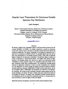
(a)

(b) Μ Ω1

mechanical modes

Ω2

Ωn

D1

optical modes

D2

Dn

laser driving .

FIG. 1. (Color online) Original Huygens’ sketch [1] of two synchronizing pendulum clocks (a) and the quantum mechanical analogue consisting of two (or more) coupled opto-mechanical systems (b). Here, mechanical resonators are driven into self-sustained oscillations by the non-linear radiation pressure force of independent optical modes. A weak mechanical interaction is responsible for the spontaneous synchronization of the limit cycles. All symbols are defined in the main text.

driving [18–21]. Such devices have all the properties (non-linear dynamics, limit cycles, etc.) which are necessary for the emergence of spontaneous synchronization [9, 22] and indeed some first experimental evidences of this effect have been found [14, 15, 17]. Quantum synchronization measures:– In a purely classical setting, synchronization is mostly studied in the context of autonomous non-linear systems undergoing limit cycles or chaotic evolution (linear systems being usually excluded because they converge to constant or unstable solutions). In this scenario one can identify different forms of synchronization [2]. Complete synchronization is achieved when (say) two subsystems S1 and S2 , initialized into independent configurations, acquire identical trajectories under the effects of mutual interactions. Specifically, given two CV classical systems characterized by the (dimensionless) canonical variables q1 (t), p1 (t) and q2 (t), p2 (t) describing the evolution of S1 and S2 in phase space, complete synchronization√is reached when the quantities√q− (t) := [q1 (t) − q2 (t)]/ 2 and p− (t) := [p1 (t) − p2 (t)]/ 2 asymptotically vanish for large enough times [23]. Phase synchronization is instead

2 achieved when, under the same conditions detailed above, only the phases ϕj (t) = arctan[pj (t)/qj (t)] are locked: i.e. when the quantity ϕ− (t) := ϕ1 (t) − ϕ2 (t) asymptotically converges to a constant phase shift ϕ0 ∈ [0, 2π]. One can already foresee that extending the above concepts to quantum mechanical systems is not straightforward and that some fundamental limits could exist that prevent the exact fulfillment of the conditions given above. In particular, identifying the dimensionless quantities qj (t), pj (t) as quadrature operators obeying the canonical commutation rules [qj (t), pj 0 (t)] = iδjj 0 [3], the relative coordinates q− (t) and p− (t) will correspond to generalized position and momentum operators of the same (anti-symmetric) mode of the system. Accordingly the uncertainty principle will now prevent the possibility of exactly achieving the condition required by classical complete synchronization. To turn this into a quantitative statement, we identify q− (t) and p− (t) as synchronization errors and introduce the following figure of merit Sc (t) := hq− (t)2 + p− (t)2 i−1 ,

(1)

gauging the level of quantum complete synchronization attained by the system (here h· · · i implies taking the expectation value with respect to the density matrix of the quantum system). We then observe that the Heisenberg principle requires hq− (t)2 ihp− (t)2 i ≥ 1/4 and hence 1

≤ 1, Sc (t) ≤ p 2 hq− (t)2 ihp− (t)2 i

(2)

which sets a universal limit to the complete synchronization two CV systems can reach. On the contrary, in a purely classical theory, Sc (t) is in principle unbounded [24]. Indeed in real units the right-hand side of the bound scales as ¯h−1 , diverging in the limit ¯h → 0. A small value of Sc (t) can have two possible origins: the mean values of q− (t) and p− (t) are not exactly zero, and/or the variances of such operators are large. The former situation can be interpreted as a classical systematic error [25], while the latter is due to the influence of thermal and quantum noise. The classical systematic error can be easily excluded from the measure of synchronization by using the same expression of Eq. (1) but after the application of the change of variables q− (t) → q− (t)−hq− (t)i,

p− (t) → p− (t)−hp− (t)i . (3)

This gives a relative measure of synchronization which is always larger than the previous absolute one and which may be preferable whenever the aim is that of selectively investigating purely quantum mechanical effects. Obviously, the bound of Eq. (2) holds also for this relative measure. Constructing a quantum analogue of the phase synchronization condition is more demanding due to the controversial nature of the quantum phase operator(s),

see e.g. Ref. [26]. In principle one could use a phasedifference operator as the one proposed in [27], however we adopt a more pragmatic approach which allows us to target departures from the ideal (classical) synchronization condition, due to quantum fluctuations. √ To do so, we write the operator aj (t) := [qj (t) + ipj (t)]/ 2 of the j-th system as aj (t) = [rj (t) + a0j (t)]eiϕj (t) ,

(4)

where rj (t) and ϕj (t) are the amplitude and phase of the expectation value of aj (t), i.e. haj (t)i = rj (t)eiϕj (t) . With this choice, the Hermitian √ and anti-Hermitian part of a0j (t) = [qj0 (t) + ip0j (t)]/ 2 can now be interpreted as fluctuations of the amplitude and of the phase respectively (indeed this is the reason why in quantum optics qj0 (t) and p0j (t) are often called amplitude and phase quadratures). If two CV systems are on average synchronized such that the phases of ha1 (t)i and of ha2 (t)i are locked, then the phase shift with respect to this locking condition can √ be associated to the operator p0− (t) = [p01 (t) − p02 (t)]/ 2. A measure of quantum phase synchronization can then be obtained through the quantity Sp (t) :=

1 0 hp (t)2 i−1 . 2 −

(5)

Differently from the measure (1), Sp can be in principle arbitrarily large. Nonetheless, if two CV quantum systems evolve in time such that their P -function [3, 28] is always positive (quantum optics notion of classicality), then perfect phase synchronization is impossible and one has positive P -function ⇒ Sp (t) ≤ 1 .

(6)

Indeed a value of hp0− (t)2 i below 1/2 implies the existence of collective squeezing and so the impossibility of a phase space representation of the state through a positive Pfunction. Notice that, with respect to the fundamental bound (2), the threshold (6) is much weaker since it can be overcome with squeezed states. Furthermore the specific structure of the limit cycles associated with the average quantities rj (t) and ϕj (t) may lead to additional bounds for Sp . If, for example, i) the system under consideration exhibits mean values quantities haj (t)i converging to approximately circular limit cycles in the phase space, ii) the noise operating in the system is not phase sensitive (i.e. is invariant for phase space rotations) and iii) the interaction potential between the two systems is of the form Hint = −µ(a1 a†2 + a2 a†1 ); then it is reasonable to conjecture that hp0− (t)2 i ≥ 0 hq− (t)2 i. This together with the Heisenberg principle, leads to the bound Sp (t) ≤ Sc (t) ≤ 1 .

(7)

3 While referring to the Supplemental Material for an heuristic derivation of Eq. (7), we remark that such inequality is consistent with the results shown later on opto-mechanical systems.

a phonon tunneling term [9] of intensity µ: X H= [−∆j a†j aj + ωj b†j bj − ga†j aj (bj + b†j ) j=1,2

+iE(aj − a†j )] − µ(b1 b†2 + b†2 b1 ). Quantum correlations and synchronization: – Synchronization and entanglement are both associated with the presence of correlations between two or more systems. It is thus natural to ask if, in the quantum regime, there is a strong interplay between the two effects. Quite surprisingly however it turns out that, according to our measures, the stationary state of two CV systems can possess maximum amount of complete or phase synchronization without being necessarily entangled. For instance a system converging to two factorized coherent states evolving in time such that ha1 (t)i = ha2 (t)i, exhibits maximum complete synchronization (Sc = 1) but has no entanglement. Similarly consider two locally squeezed states rotating in phase space such that ha1 (t)i = ha2 (t)i and hp01 (t)2 i = hp02 (t)2 i = , with p0k being the quadrature orthogonal to the phase space cycle of subsystem k as defined in Eq. (4) (said in simpler words, these are two squeezed states moving like synchronized clock hands in phase space). This state has arbitrary high phase synchronization Sp = 21 −1 but it is clearly not entangled. Entanglement appears hence to enforce correlations which are qualitatively different from those required to yield high values for Sc (t) and Sp (t). A better insight on this can be obtained by considering the very precursor of all CV entangled states, i.e. the EPR state [33] which describes the ideal scenario of two systems having same positions but opposite momenta. It is thus clear that synchronization requires different constraints which could have instead a relationship with other measures of quantum correlations like quantum discord (see e.g. our successive results on opto-mechanical systems). We conclude this section with an open question on the converse problem: what kind of synchronization phenomenon corresponds in the quantum limit to EPR correlations? EPR entanglement could be identified as a mixture of complete and anti-synchronization, i.e. q1 (t) = q2 (t) and p1 (t) = −p2 (t). Recently this unconventional regime called mixed synchronization has been introduced and observed in classical non-linear systems [34], but whether this concept is relevant and extendible in the quantum domain is still unexplored.

Measures and bounds at work:– Opto-mechanical devices [4, 5] provide the perfect setting where our measures for synchronization can be directly applied. We thus identify S1 and S2 with two approximately identical mechanical resonators (see Fig. 1.b) coupled to independent cavity optical modes (needed to induce selfsustained limit cycles) and mutually interacting through

(8)

In this expression, for j = 1, 2, aj and bj are the optical and mechanical annihilation operators, ωj are the mechanical frequencies, ∆j are the optical detunings, g is the opto-mechanical coupling constant, while E is the laser intensity which drives the optical cavities (¯h = 1). For simplicity g and E are assumed to be equal in both systems while ω1 and ω2 can be slightly different. Dissipative effects are included adopting the Heisenberg picture and writing the following quantum Langevin equations [29], √ a˙ j = [−κ + i∆j + ig(bj + b†j )]aj + E + 2κain j , (9) p ˙bj = [−γ − iωj ]bj + iga† aj + iµb3−j + 2γbin . j j Here κ and γ are, respectively, the optical and mein chanical damping rates while ain j and bj are the input bath operators. These are assumed to be white Gaussian fields obeying standard correlation relations, † in 0 in 0 in † 0 hain j (t) aj 0 (t ) + aj 0 (t )aj (t) i = δjj 0 δ(t − t ) and † in 0 in 0 in † 0 hbin j (t) bj 0 (t ) + bj 0 (t )bj (t) i = (2nb + 1)δjj 0 δ(t − t ), h ¯ω

where nb = [exp( kB Tj ) − 1]−1 is the mean occupation number of the mechanical baths which gauges the temperature T of the system [29] (since we are only interested in the situation in which ω1 ' ω2 , the parameter nb can be safely taken to be equal for both oscillators). The operators O(t) in Eq. (9) can be expressed as sums of mean values hO(t)i plus fluctuation terms O0 (t), i.e. we write O(t) = hO(t)i + O0 (t). In a semiclassical approximation [29] we determine the expectation values hO(t)i in terms of a set of classical non-linear differential equations and, as a second step, we linearize the quantum Langevin equations for the operators O0 (t). Setting ∆j = ωj (driving detuning) and choosing the laser amplitude E of Eq. (8) large enough, we make sure that such solutions yield limit cycles as classical steady state configurations (see e.g. [30]). In this regime the mechanical and optical fileds acquire large coherent amplitudes and therefore we expect the linearization procedure to be justified. A more general and exact treatment of the non-linear dynamics could be achieved by using stochastic methods like those presented in Ref.s [35, 36]. Quantum fluctuations are obtained by computing the covariance matrix C(t), with entries given by Ci,` (t) = hRi (t)R` (t)† + R` (t)† Ri (t)i/2, the expectation value being taken on the initial state and Ri being the compo0† 0 0† 0 0† 0 nents of the vector R = (a01 , a0† 1 , b1 , b1 , a2 , a2 , b2 , b2 ). In particular this gives us direct access to the mechanical variances hq− (t)2 i and hp− (t)2 i which define the complete synchronization level via Eq.(1). By applying the linearization procedure, we implicitly performed the change

4

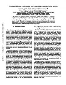
0.25 0.20 0.15 0.10 0.05 0.00

HbL Sc , S p , DG

Sc, S p

HaL

0 100 200 300 400 500 600 tΤ

0.25 æ 0.20 æ 0.15 à æ à 0.10 0.05 à ì ì æ à ì 0.00 ì 0.00 0.01

æ æ æ æ æ

æ æ æ

à

æ à à æ æ æ æ æ à à à à à æ à

à

5

10 nb

æ

0.02 Μ

0.03

0.04

HdL

15

20

Sc , S p

0.25 0.20 à 0.15 0.10 0.05 0.00 0

æ

à à à à ì ì à à à ì ì ì ì ì

HcL æ

Sc , S p

of variables corresponding to Eq. (3) and so we automatically excluded the systematic synchronization error due to slightly different average trajectories. As a consequence the only source of disturbance bounding our measure of synchronization will be quantum (or thermal) fluctuations. Estimating phase synchronization as in Eq.(5) requires instead a further step as the latter has been defined with respect to a reference frame rotating with the phases of the average trajectories, see Eq. (4). This corresponds to a diagonal and unitary operation on R, built up on the phases ϕa1 (t) = argha1 (t)i, ϕa2 (t) = argha2 (t)i, etc., of the classical orbits: i.e. R → R0 = U (t)R with U (t) = diag[e−iϕa1 (t) , eiϕa1 (t) , · · · ]. The associated covariance matrix is C 0 (t) = U (t)C(t)U (t)† , from which we can directly extract the mechanical variance hp02 − (t)i entering Eq.(5). A simulation of the complete and phase synchronization between the mechanical modes is plotted in Fig. 2.a using realistic values for the parameters [4, 5] (see caption for details). After an initial transient, the system reaches a periodic steady state in which Sc (t) and Sp (t) are significantly larger then zero, implying that both complete and phase synchronization take place in the system. Their value is consistent with the fundamental limit (2) imposed by the Heisenberg principle and with the heuristic bound (7) presented in the previous section. Indeed we numerically find that quantum squeezing in the p0− (t) quadrature, needed to overcome the non-classicality threshold (6), is absent in the system. Fig. 2.b and Fig. 2.c report instead the behavior of the time averaged measures of complete and phase synchronization for different values of the coupling constant and of the bath temperature. We vary µ from zero [31] to a maximum threshold above which the classical equations are perturbed too much destroying the limit cycles. Finally we have checked if quantum correlations are present in the system verifying that, consistently with the difference between entanglement and synchronization detailed in the previous section, for many choices of the parameters entanglement negativity is always zero even though synchronization is reached. On the contrary, nonzero level of Gaussian quantum discord [32] (Fig. 2.b) between the two mechanical modes is observed for all values of µ that lead to synchronization. Still our data are not sufficient to clarify the functional relationship between discord and synchronization (if exists). The synchronization observed between the oscillators is expected to emerge also when more than two parties are present in the setup. In particular we focus on the case of a (closed) chain formed by N opto-mechanical systems with first neighbor interactions (the Hamiltonian being the natural generalization of (8) with uniform parameters). As before, we enforce the driving detuning condition ∆ = ω and set the laser intensities E in order that each opto-mechanical system converges to a stable

0.25 0.20 0.15 0.10 0.05 0.00 0

æ

à

æ æ à à

2

æ æ æ à à à æ æ æ æ à à à à

4

6

8

10

h

FIG. 2. (Color online) Subfigure (a): simulation of the complete (blue) and phase (green) synchronization measures (1) and (5) between the mechanical resonators as functions of time (in units of τ = 2π/ω1 ). The dashed lines indicate the corresponding time averaged asymptotic values, i.e. the quanRT tities S¯x = limT →∞ T1 0 Sx (t)dt for x = c, p. Setting ω1 = 1 as a reference unit of frequency, the other physical parameters which have been used in the simulation are: ω2 = 1.005, γ = 0.005, ∆j = ωj , κ = 0.15, g = 0.005, µ = 0.02, nb = 0 and E = 320. Subfigure (b): time averaged complete (circles) and phase (squares) synchronization and Gaussian discord DG (diamonds) as functions of the coupling constant µ. Subfigure (c): time averaged synchronization measures as functions of the bath mean phonon number nb . Subfigure (d): Synchronization between two arbitrary mechanical modes of a chain of 20 coupled opto-mechanical systems as a function of the lattice distance h. All subsystems are assumed to have the same mechanical frequency ω = 1.

limit-cycle. Once these prerequisites are fulfilled we linearize the dynamics around the classical steady state, which is assumed to be the same (synchronized) in each site, i.e. haj (t)i = α(t) and hbj (t)i = β(t) for all j. This corresponds to a mean-field approximation applied only to the classical dynamics, while the fluctuation terms a0j and b0j can be treated exactly (without mean-field) since the associated Hamiltonian is quadratic. Fig. 2.d reports the results obtained for two mechanical modes separated by h lattice steps: we notice that the synchronization level among the various elements persists even if an exponential decay in h is present (a behavior which is consistent with the one-dimensional topology induced by the selected interactions). Summary: – We have quantitatively studied the phenomenon of spontaneous synchronization in the setting of coupled CV quantum systems. We have shown that quantum mechanics sets universal limits to the level of synchronization and discussed the relationship between this phenomenon and the emergence of quantum correlations. Finally we have analyzed the spontaneous synchronization of opto-mechanical arrays driven into self-

5 sustained oscillations. A large number of open aspects are worth being further investigated, among which: the interplay between quantum correlations and synchronization, the application of this theory to other physical systems like coupled optical cavities [16], self-locking lasers [37], etc. and the interpretation of synchronization as a useful resource for quantum communication and quantum control. Acknowledgments. – This work has been supported by IP-SIQS, PRIN-MIUR and SNS (Giovani Ricercatori 2013). N.D. acknowledges support from CIFAR.

[1] C. Huygens, Œuvres Compl`etes de Christiaan Huygens, vol. 15 pp. 243 (1893) Martinus Nijhoff, The Hague; ibid. vol. 17 pp. 183 (1932). [2] A. Pikovsky, M. Rosenblum and J. Kurths, Synchronization: A Universal Concept in Nonlinear Sciences, Cambridge University Press, New York (2001). [3] S. L. Braunstein and P. van Loock, Rev. Mod. Phys. 77, 513 (2005); C. Weedbrook et al., Rev. Mod. Phys. 84, 621 (2012); A. Ferraro, S. Olivares and M. G. A. Paris, Gaussian states in continuous variable quantum information, (Bibliopolis, Napoli) (2005). [4] F. Marquardt, S. M. Girvin, Physics 2, 40 (2009). [5] M. Aspelmeyer, T. J. Kippenberg, F. Marquardt, arXiv:1303.0733, (2013). [6] V. Giovannetti, S. Lloyd, L. Maccone, J. H. Shapiro and F. N. C. Wong, Phys. Rev. A 70, 043808 (2004); R. Jozsa, D. S. Abrams, J. P. Dowling, and C. P. Williams, Phys. Rev. Lett. 85, 2010 (2000); I. L. Chuang, Phys. Rev. Lett. 85, 2006 (2000); V. Giovannetti, S. Lloyd, and L. Maccone, Nature 412, 417-419 (2001). [7] O. V. Zhirov and D. L. Shepelyansky, Phys. Rev. Lett. 100, 014101 (2008); S.-B. Shim, M. Imboden and P. Mohanty, Science 316, 95 (2007). [8] I. Goychuk, J. Casado-Pascual, M. Morillo, J. Lehmann, and P. H¨ anggi, Phys. Rev. Lett. 97, 210601 (2006). [9] M. Ludwig and F. Marquardt, Eprint arXiv:1208.0327 [quant-ph] (2012). [10] U. Akram and G. Milburn, AIP Conf. Proc. 1363, 367 (2010). [11] A. Tomadin, S. Diehl, M. D. Lukin, P. Rabl and P. Zoller, Phys. Rev. A 86, 033821 (2012). [12] G. L. Giorgi, F. Galve, G. Manzano, P. Colet and R. Zambrini, Phys. Rev. A 85, 052101 (2012); G. Manzano, F. Galve, G. L. Giorgi, E. Hern` andez-Garc´ıa and R. Zambrini, Sci. Rep. 3, 1439 (2013). [13] O. V. Zhirov and D. L. Shepelyansky, Eur. Phys. J. D 38, 375 (2006). [14] S. Shim, M. Imboden, P. Mohanty, Science 316, 95 (2007). [15] M. Zhang et al., Phys. Rev. Lett. 109, 233906 (2012). [16] T. E. Lee and M. C. Cross, arXiv:1209.0742, (2012). [17] M. H. Matheny et al., arXiv:1305.0815, (2013). [18] E. Buks and M. L. Roukes, J. of Microel. Sys. 11, 6 (2005). [19] Q. Lin et al., Nature Photonics 4, 236 (2010). [20] M. Eichenfield, R. Camacho, J. Chan, K. J. Vahala and O. Painter, Nature 462, 78 (2009).

[21] D. E. Chang, A. H. Safavi-Naeini, M. Hafezi and O. Painter, New J. Phys. 13, 023003 (2011). [22] G. Heinrich, M. Ludwig, J. Qian, B. Kubala and F. Marquardt, Phys. Rev. Lett. 107, √ 043603 (2011). [23] The normalization factor 2 is introduced for a convenient notation in the quantization of the system. [24] In a purely classical setting, h· · · i of Eq. (1) accounts for taking the average over several realization of the stochastic process that tamper the system, or equivalently with respect to a time dependent phase space distribution. Notice that in this case, to put our definitions on a solid theoretical ground, the variables qj (t), pj (t) need to be not just dimensionless (fundamental requirement to introduce ϕj (t)) but also properly normalized in order to remove any ambiguity in the sum at the rhs of Eq. (1). For the models we are dealing with, i.e. systems of coupled harmonic oscillators, this can be easily done by ensuring that when moving into the quantum domain the observables associated with qj and pj will allow us to express the local Hamiltonian as Hj = ¯ hωj (p2j + qj2 )/2 (ωj being the corresponding frequencies). [25] If the averaged phase-space trajectories (limit cycles) of the two systems are constant but slightly different from each other, it means that this kind of error is not due to random noise but it is instead systematic. With the term systematic we mean that, with many measurements, this average error can be estimated and subtracted from the measured data in order to single out the pure effect of quantum noise on the amount of synchronization. [26] M. Ban, Phys. Lett. A 199 275 (1995). [27] A. Luis and L. L. Sanchez-Soto, Phys. Rev. A 48, 4702 (1993). [28] R. J. Glauber, Phys. Rev. 131, 2766 (1963). [29] D. Vitali, S. Mancini, L. Ribichini and P. Tombesi, Phys. Rev. A 65, 063803 (2002); A. Mari and J. Eisert, Phys. Rev. Lett. 103, 213603 (2009); A. Farace and V. Giovannetti, Phys. Rev. A 86, 013820 (2012). [30] F. Marquardt, J. G. E. Harris and S. M. Girvin, Phys. Rev. Lett. 96, 103901 (2006); M. Ludwig, B. Kubala and F. Marquardt, New J. of Phys. 10, 095013 (2008). [31] For µ = 0, the two resonators asymptotically acquire independent phases diffused along the respective limit cycles of radius R ' 500 (with parameters of Fig. 2). In this case we can estimate Sc = 2hq12 + p21 + q22 + p22 i−1 ' R−2 ' 4 × 10−5 . [32] G. Adesso and A. Datta, Phys. Rev. Lett. 105, 030501 (2010). [33] A. Einstein, B. Podolsky, and N. Rosen, Phys. Rev. 47, 777 (1935). [34] A. Prasad, Chaos Solitons Fractals 43, 42 (2010); A. Sharma and M. D. Shrimali, Nonlinear Dyn. 69, 371 (2012); K. Czolczynski, P. Perlikowski, A. Stefanski and T. Kapitaniak, Commun. Nonlinear Sci. Numer. Simulat. 17, 3658 (2012). [35] P. D. Drummond and C. W. Gardiner, J. Phys. A 13, 2353 (1980). [36] K. Dechoum et al., Phys. Rev. A 70, 053807 (2004). [37] R. Graham, Springer Tracts in Mod. Phys. 66, (1973).

6 SUPPLEMENTAL MATERIAL: HEURISTIC BOUND TO PHASE SYNCHRONIZATION

The hypothesis underlying the conjecture (7) are: (i) the system admits limit cycles which are approximately circular haj (t)i ' rj e−iωt , (ii) thermal (or quantum) noise is not phase sensitive in the sense that it is invariant for phase space rotations, and (iii) the interaction potential between the two systems is of the form Hint = −µ(a1 a†2 + a2 a†1 ). These assumptions are often valid for optical or mehcanical modes under the rotating wave approximation. For such systems the interaction can be written in terms of symmetric and anti-symmetric normal modes Hint = −µa†+ a+ + µa†− a− which up to a renormalization of the bare frequencies (ω → ω − µ) 0 is equivalent to Hint = 2µa†− a− . This means that, because of the interaction, the anti-symmetric mode rotates with a frequency 2µ faster with respect to the symmetric mode. Since the phase of each individual limit cycle is arbitrary, the same must be true for the symmetric mode. Unless anti-synchronization appears, one can guess the following structure for the linearized equations for the

fluctuations:  0    0  d q+ −γef f 0 q+ = + noise. 0 0 p0+ dt p0+

(10)

The reason is that the symmetric mode must be stable in the amplitude (with effective damping γef f > 0) but its phase should be completely free to diffuse (the corresponding Lyapunov exponent must be zero). The dynamics of the anti-symmetric mode, linearized around a synchronized solution, will be like Eq. (10) plus a frequency shift of 2µ due to the interaction potential:  0    0  d q− −γef f −2µ q− = + noise. (11) 0 0 p 2µ 0 p dt − − The new matrix, for µ 6= 0, has negative eigenvalues and this fact is the origin of synchronization. Since we assumed the noise to be phase insensitive the diffusion matrix must be proportional to the identity. In this case one can easily find the steady state and check that in0 0 deed hp−2 i ≥ hq−2 i, and hence the bound (7) holds. Of course this heuristic argument is very hand-waving but it gives the physical intuition that, in a classical or quantum system, the precision of phase synchronization may be bounded by the precision of amplitude synchronization.