Measuring Significance of Community Structure in Complex Networks Yanqing Hu∗ , Yuchao Nie, Hua Yang, Jie Cheng, Ying Fan and Zengru Di†
arXiv:0902.3331v1 [physics.soc-ph] 19 Feb 2009
Department of Systems Science, School of Management, Center for Complexity Research, Beijing Normal University, Beijing 100875, China Many complex systems can be represented as networks and separating a network into communities could simplify the functional analysis considerably. Recently, many approaches have been proposed for finding communities, but none of them can evaluate the communities found are significant or trivial definitely. In this paper, we propose an index to evaluate the significance of communities in networks. The index is based on comparing the similarity between the original community structure in network and the community structure of the network after perturbed, and is defined by integrating all the similarities. Many artificial networks and real-world networks are tested. The results show that the index is independent from the size of network and the number of communities. Moreover, we find the clear communities always exist in social networks, but don’t find significative communities in proteins interaction networks and metabolic networks. PACS numbers: 89.75.Hc, 87.23.Ge, 89.20.Hh, 05.10.-a
The study of the community structure of networks has become a very important part of researches of complex networks. Nodes belonging to a tight-knit community are more likely to have particular properties in common. In social relationship network, communities usually represent different friend subgroups. In the world wide web, community analysis has uncovered thematic clusters. In biochemical or neural networks, different communities may represent different functional groups, and separating the network into such groups could simplify the functional analysis considerably. As a result, the problem of identification of communities has been the focus of many recent efforts. So two questions are proposed, the first is, how to detected communities in the networks? In recent studies, plenty of algorithms are proposed [1, 2, 3, 4, 5, 6, 7, 8, 9, 10, 11, 12, 13, 14, 15] (see [5] as a review). The second question is coming hand in hand with the first question: how to evaluate the communities detected? We believe that there exist clear communities in some networks while no clear communities in the other networks. But almost all algorithms could find the “community structure” in networks in their ways, without thinking about whether the community structure actually exists or not. Even many algorithms can also find the community in random networks, in which are considered having no community. For the existence of such a situation, the discussion on the “significative communities” is needed. As a network is given, it is meaningless to detect the community when the community structure is not significative at all. Scientists try to propose a universal index to evaluate the partitions. And the modularity Q [16] was presented as an index of community structure and by now it has been widely accepted [5, 10, 11, 14] as a measure for the community structure. Modularity Q was presented as
∗
[email protected] †
[email protected]
a index of community structurePby Newman and Grive, which was introduced as Q = r (err − a2r ), where err are the fraction of links that connect two nodes inside the community r, ar the fraction of links that have on or both vertices in side the community r, and sum extends to all communities r in a given network. The larger the value of Q is, the more clearly a partition into communities is. Hence, the value of the modularity can be used as a significative index for communities. Unfortunately, despite the obvious advantages of modularity, it has its own problem. It is true that networks with strong community structure have high modularity but not all networks with high modularity have strong community structure [18]. Here, we just say Q value is not a very good index to evaluate the significance of community structure, but do no mean that maximizing modularity Q cannot detect community structure. Many empirical and numerical results represent maximizing modularity Q is a good method for detecting communities [5, 10, 14]. Therefore in the following analysis, we still use maximizing modularity Q to detect community structure. Recently, Karrer, Levina, and Newman have suggested a method to perturb the networks. They have shown some phenomena about the robustness of community structure in networks [17]. Intuitively, if a network has distinct communities, the community structure should be robust under perturbation. Thus in this paper, we develop a perturbation method and propose an index to measure the significance of communities based on the perturbation to the network, and try to solve the second question mentioned above. In our method, we strengthen the perturbation to the network from just small amount of edges rewired to all edges rewired. Then we can get the results of perturbations (the similarity of community structure between original and perturbed networks) for each case. Finally we get our index by integrating all the similarities of perturbations. Using our index, we can evaluate whether the network has a “significative communities”. The method is described in detail in the following section. Naturally, we apply the method to many
2 kinds of networks, and find some interesting conclusions. We argue that social networks usually have distinct and significative community structure, while metabolic networks also have community structure but not so clear. However, some protein interaction networks we tested have no significant communities.
I.
METHOD
There are three steps to get our index for a given network. First, we detect the communities in the original network without any perturbation. Second, we will perturb the network, using the way of perturbing the edges in network by an arbitrary amount. Then we can detect the new communities after perturbation. Besides, we calculate the similarity between the two partitions (the communities of original network and perturbed network). Third, we increase the proportion of edges perturbed little by little until all edges are perturbed, repeat the process of second step, and compare the new communities with original ones with perturbation strengthened. Hence, we can get a series of proportion of perturbation as well as the corresponding similarity values. At last, we sum up all the products of similarity values and the corresponding increased proportion of perturbation. If we just increase the proportion little enough, the process just like the calculation of integration. When we perturb the edges in the network, there are various methods to achieve. In this paper, we adopt absolutely random perturbation to the network. Consulting to the method of network perturbation introduced by Newman [17], we makes sure the total number of edges is unchanged, which make the comparison of the partitions straightforward. Specifically, we go through each edge in original network and with probability p we remove it, then we add the same amount of edges randomly between any two nodes, which have no connection after perturbation. In this way, if p=0, no edge is moved and the network is all the same with original. If p=1, all edges are moved and the process generates a random graph, which has no correlation with original. And for values of p between 0 and 1 the perturbation generates networks in which some of the edges retain their original positions while the others are moved to new positions. Therefore, we adopt a sequence perturbation to the network. We do not only perturb networks by little, but also strengthen the proportion of perturbation until all the edges move their positions. Further, we do not care if the expected average degrees of every node is the same as before, which is different from Karrer and Newman et al[17]. We argue that the absolutely random perturbation to the network is more reasonable, simple and efficient. After detecting the community structure in the networks perturbed, the question becomes how to compare the similarity between the communities perturbed and the original. We think that a more discriminatory measure is the normalized mutual information index, which
is based on information theory, as described in Ref [19]. They defines a confusion matrix N , where the rows correspond to the “real” communities in networks without perturbation, and the columns correspond to the “found” communities. The element of N , Nij is the number of nodes in the real community i that appear in the found community j. Therefore a measure of similarity between the partitions A and B is PcA PcB Nij N −2 i=1 j=1 Nij log( Ni. N.j ) I(A, B) = PcA (1) PcB N.j Ni. i=1 Ni. log( N ) + j=1 N.j log( N )
As the discrepancy of partitions increases, the value of I(A, B) decreases from 1. In this paper, we compare the “communities without perturbation” A and the “communities after perturbation” A(p), what is different, we make a little change on the similarity index. We found that the I(A, A(p)) has been not only decided by the discrepancy of the communities, but also influenced by the size of networks and the number of community in A and A(p). In order to eliminate the influence of the size, we consider the improved measure below: S(A, A(p)) = I(A, A(p)) − I(Arand , Arand (p))
(2)
where, Arand or Arand (p) has same number of communities with A or A(p), moreover each community in Arand or Arand (p) has the same number of nodes with the corresponding community in A or A(p) respectively. But different from A, A(p) that are correlated with the original network, the nodes in Arand and Arand (p) are randomly selected form the whole set of nodes. In this way, we can get a series of values of S(A, A(p)) by strengthening the proportion of perturbations from 0 to 1 little by little. We adopt 0.02 as the increased proportion of perturbation for each time in this paper. Generally, a higher proportion of perturbation corresponding to a lower value of S(A, A(p)). Hence,we can get our measure as following: Z 1 S(p)dp (3) R= 0
where p is the proportion of perturbation, and S(p) is the similarity value between original community structrue and the community sturcture when the proportion of perturbation is p. If a network has distinct community structure, the value of our measure R is inclined to high. On the contrary, the network holding fuzzy community structure displays low value. For a random network R will approach to 0 theoretically. The value of the similarity is a function of the parameter p that measures the amount of perturbation. The similarity value starts at 1 when p = 0, as we would expect for an unperturbed network. Then the similarity value drops off and approaches its minimum value while p = 1, while the network at present is an absolute random network. Dose the measurement is independent with the size of network, and what will happen when changeing the number of communities with same size and number of edges?
3 1 0.8 1000n 2c 500n 2c 100n 2c 1000n 3c 500n 3c 100n 3c 1000n 4c 500n 4c 100n 4c
R
0.6 0.4 0.2 0 0
50
100 150 Average degree
1
BA 1000n Q BA 1000n R BA 500n Q BA 500n R BA 100n Q BA 100n R ER 1000n Q ER 1000n R ER 500n Q ER 500n R ER 100n Q ER 100n R
0.8 0.6 0.4 0.2
II.
200
FIG. 1: The relationship among the value of R index, network size average degree and community number. In the plot ‘xn yc’ denotes x nodes and y pre-determined communities with same size. Every pre-determined communities (sub-networks) are generated by the same way. They are ER networks and disconnected with each other. From the plot we can see that the value of R increase with the increasing of average degree and is almost independent from the size of network and number of communities.
R
Moreover, can the measurement work well in some networks that Q index fails to measure [18]? In order to give answers to the above questions, firstly we apply the measurement R in same size networks with same number of communities, and each community with same number of nodes. There are no edge between different sub-networks and each of them is ER network. That means the communities are distinct. Numerical experiments present that, the value of index R is roughly independent with the size of network and number of communities. When the average degree increases, the value of R will increase correspondingly (as shown in Fig. 1). Secondly, we compare Q index and R index in ER networks. It is known that Q index cannot measure ER and BA networks [18]. For the BA and ER networks with lower average degree, the modularity Q could be very high. So we compare R index with Q index in different BA and ER networks with different size and average degree. The results tell us that R index has the same behaviors in BA and ER networks. When the average degree is large or equal to 2, R index will be lower than 0.1, and soon be stable. When the average degree is 1, the R is less than 0.2. From the following applications on artificial networks (as shown in Fig. 3), we known that R < 0.1 is a low value. It indicates there are no community structure in the network. But R = 0.2 is not very low. It presents there exists fuzzy communities in the network. Hence, our index performs well but it is also not suitable for some networks where average degree is less than 1. Fortunately, there are few real-world networks with average degree less than 1. By and large, our index is more efficient than Q index in BA and ER networks (as shown in Fig. 2). Moreover, from the numerical experiments we find that for a very large size network which contains two equal clique-complete community structure network, the value R can be larger than 0.9, and the value of R can lower than 0.03 for large size random networks with proper average degree. Thus, we can conclude that R ∈ (0, 1) roughly.
RESULT 0 0
In order to test the validity of our index. Firstly, we apply it on computer-generated random networks with a well-known predetermined community structure. Each network has n = 128 nodes divided into 4 communities of 32 nodes each. Edges between two nodes are introduced with different probabilities depending on whether the two nodes belong to the same community or not: every node has hkin i links on average to its fellows in the same community, and hkout i links to the other communities, keeping hkin i + hkout i = 16. As is known to all, the communities become more and more diffuse and harder to identify when kout increase, hence the significance of the communities found by algorithm also tends to weakness and R index will decrease. In order to validate the expectation that R index will become lower as the kout decreases, we calculate the value of R in the case that
10
20 30 Average degree
40
50
FIG. 2: Comparing modularity Q and index R in BA and ER networks in which there exists no community structure. From the plot we can see that, Q is very large when the average degree is about 1, while, value of R is near 0.2. That is to say, when average degree is near 1, Q index presents very strong community structure, and R shows fuzzy community structure (we obtain that there exits fuzzy community structure when R = 0.2 form the numerical results in artificial networks (see Fig. 3)). But when the average degree increases, Q drops more slowly than R. When the average degree is larger or equal to 2, R is very low and achieves stable state soon, which indicates R index perform well in both BA and ER networks.
4
0.5
R
0.4 0.3 0.2 0.1 0 0
2
4
6 8 outdegree
10
12
FIG. 3: The x-axis is kout (the proportion of connections between communities),while the y-axis represents the value of measurement as described in this paper. The percentage we increase the proportion of perturbation is 0.02 for each time. Each value corresponding to the kout is the average value of 20 numerical experiments where each time we generate a new independent network. The value of R is 0.58 when kout is 0 but R is 0.05 when kout is 11. When kout is about 11, the network is random in which there is no community structure theoretically.
kout ranges from 0 to 12. The method we use to detect community structure in this paper is the combination of Newman’s spectral algorithm and extremal optimization algorithm [10, 14]. We use spectral algorithm to detect the initial community structure, and extremal optimization algorithm to improve the community partition. We also use an other algorithms [20] to detect the community structure, we find the influence of different algorithms on our index is neglectable. The result is shown in Fig.3. As our anticipation, the value of index varies from 0.58 to 0.05 as kout varies from 0 to 12, which means that our index have good ability to mark the significative of communities in computegenerated network. For larger values of kout , the value of the index is lower, indicating that the community structure is not more significative than that of a random graph. The index decreases as a function of kout , indicating that the community structure discovered by the algorithm is relatively significative when kout is relatively low (or kin is relatively high). Of course, we also apply it on many real networks [21, 22, 23, 24, 25, 26, 27, 28, 29]. A good index shouldn’t be available to computer-generated networks only, but also has good behavior in real networks. It is necessary to proof-test our index on all kinds of real networks. People usually classify the real networks into three sorts: social networks (such as scientist collaborations and friendships), biological networks (such as proteins interaction networks and metabolic networks) and technological net-
works (such as Internet and the WWW). Distinct communities within networks have been observed in different kinds of networks, most notably in social networks while fuzzy in biological networks often. We apply the index into many different networks, and obtain relatively high value of our index in social networks. Therefore, we validate the availability of our index. You can get more detail form Fig.4 and Tab.I. Fig.4 shows the curves of S(p), using 4 networks as an example. Here we average the results of the 20 times simulation in the figure, in which we earmark the maximum, minimum, and the mean value of the 20 times simulation. As is shown, the similarity measure of Jazz network decrease slowly while the similarity of the other three networks decrease rapidly. The figure argues that the communities in Jazz network are more robust than other three. It means that the structure of the Jazz network is hardly changed under perturbation. Thus the community structure in Jazz network is distinct and significative. Tab.I shows all the networks we apply the index on. From the table, we find different kinds of networks have different index values, which indicate the significance of the communities in different networks varies. First, we analyze several social networks, including Zachary karate club network, dolphin network, collage football network, Jazz network, scientists collaboration network and so on. We get relatively high value of our index among these networks, and most of these networks have the index value over 0.27, which shows the existence of strong community structure in these networks, and the community structure found in these networks are clear. However, the Santa Fe scientists collaboration network has an index value 0.14, which is low. As is known, the Santa Fe Institute is different from many other Institutes. Renowned scientists and researchers that come to Santa Fe Institute are from universities, government agencies, research institutes, and private industry. Therefore the relationship between the members is not as tight as other collaboration networks. All the social networks in Tab.I are networks of friendship (collaboration could be viewed as a form of friendship). Just as said “Birds of a feather flock together”, it is easy to understand why the social networks always centralize as some distinct groups. What’s more, we also analyze some biological networks such as proteins interaction networks E.coli, Yeast and H.Sapiens, and many metabolic networks. We find in proteins interaction networks the R index value are low (the average degree of H.Sapiens is less than 2, so its R index is little high). In metabolic networks, we calculate 43 metabolic networks, all the index value R are medium about 0.19. For the average nodes’ number 1488 and average edges’ number 3460, the average index value is 0.19. Therefore we conclude that in some proteins interaction networks (such as E.coli and Yeast) and the metabolic networks which are listed in the following table, there are no clear communities. It may be unnecessary to detect and analyze the communities in these networks.
5 III.
1
E.Coli Celegans Neural Jazz Helicobacter pylori
Similarity
0.8 0.6 0.4 0.2 0 0
0.2
0.4 0.6 Disturb rate
0.8
1
FIG. 4: The x-axis represent the average number of perturbation, while the y-axis is the similarity value S(p). For each network, we earmark three value here: maximum, minimum and mean of 20 times simulation. The network in turn are proteins interaction network (E. coli), neural network (C. elegans), social network (Jazz) and metabolic network (Helicobacter Pylori) from the bottom up. The increase of he proportion of perturbation every time is 0.02
CONCLUSION AND DISCUSSION
In this paper an index is presented which can measure the significance of communities detected. The index is based on comparing the similarity between the original community structure and the community structure after perturbed in the network. Then the index value is the integration of all the similarities. We apply the index to many artificial and real world networks, such as social networks, neural network, proteins interactions networks and metabolic networks. The results show that our index is independent form the network size and community number. Moreover we find the different kinds of networks have different characteristics, social networks usually have significant communities, while communities are comparatively fuzzy in biological networks, especially in some protein-interaction networks.
TABLE I: The integral measure of some real networks. The table shows the names of different real networks and the corresponding index values. The column of size denotes the number of nodes and edges network E.coli Yeast H.Sapiens Celegans metabolic Aquifex aeolicus Helicobacter pylori Yersinia pestis 43 metabolic networks Celegans neural Santa Fe scientists Zachary karate Dolphin College football Jazz Political blogs Political books
size 1442, 5873 1870, 4480 693, 982 453, 4596 1485, 3400 1363, 3151 1950, 4505 1488, 3460 297, 2359 260, 2692 34, 78 62, 159 115, 613 198, 5484 1224, 19090 105, 441
R type 0.14 protein 0.14 0.21 0.19 metabolic 0.19 0.19 0.18 0.19 0.24 neural 0.14 social 0.27 0.27 0.38 0.42 0.29 0.34
[1] R. Albert, A.-L. Barabasi, Rev. Mod. Phys. 74, 47 (2002). [2] M. E. J. Newman, SIAM Rev. 45, 167-256 (2003). [3] M. E. J. Newman, Proc. Natl. Acad. Sci, U. S. A. 98,404 (2001) [4] L. Danon, J. Duch, A. Arenas, and A. Diaz-Guilera, arXiv:cond-mat/0505245, (2005).
Acknowledgement
This work is partially supported by 985 Project and NSFC under the grant No. 70771011, and No. 60534080.
[5] S. Lehmann and L. K. Hansen, arxiv.org/abs/physics/0701348, (2007). [6] M. Latapy and P. Pons,Proceedings of the 20th International Symposium on Computer and Information Sciences, ISCIS’05, LNCS 3733, 284-293, (2005). [7] F. Wu and B. A. Huberman, The Eur. Phys. J. B 38,331338 (2004)
6 [8] A. Clauset, Phys. Rev. E 72, 026132, (2005). [9] S. Muff, F. Rao and A. Caflisch, Phys. Rev. E 72, 056107, (2005). [10] M. E. J. Newman, Proc. Natl. Acad. Sci. USA 103, 85778582 (2006) [11] M. E. J. Newman, Phys. Rev. E 74, 036104, (2006). [12] C. P. Massen and J. P. K. Doye, Phys. Rev. E 71, 046101, (2005). [13] M. Girvan and M. E. J. Newman, Proc. Natl. Acad. Sci. U. S. A 99,7821-7826. (2004) [14] J. Duch and A. Arenas, Physical Review E , vol. 72, 027104, (2005). [15] M. E. J. Newman and E. A. Leicht, Proc. Natl. Acad. Sci. USA 104, 9564-9569 (2007). [16] M. E. J. Newman and M. Girvan, Phys.Rev.E 69, 026113 (2004) and D. Wagner, arXiv:physics/0608255, (2006) [17] B. Karrer, E. Levina, and M. E. J. Newman, Phys. Rev. E 77, 046119, (2008) [18] R. Guimer‘a, M. Sales-Pardo, and L. A. N. Amaral, Phys. Rev. E 70, 025101 (2004). [19] L. Donetti and M. A. Munoz,J. Stat. Mech. P10012 (2004)
[20] Y. Hu, M. Li, P. Zhang, Y. Fan, and Z. Di, Phys. Rev. E 78, 016115 (2008) [21] W. W. Zachary, Journal of Anthropological Research 33, 452-473 (1977). [22] D. Lusseau, K. Schneider, O. J. Boisseau, P. Haase, E. Slooten, and S. M. Dawson, Behavioral Ecology and Sociobiology 54, 396-405 (2003). [23] L. A. Adamic and N. Glance, ”The political blogosphere and the 2004 US Election”, in Proceedings of the WWW2005 Workshop on the Weblogging Ecosystem (2005). [24] D. J. Watts and S. H. Strogatz, Nature 393, 440-442 (1998). [25] P.Gleiser and L. Danon , Adv. Complex Syst.6, 565 (2003). [26] J. Duch and A. Arenas, Physical Review E , vol. 72, 027104, (2005). [27] http://www-personal.umich.edu∼mejn/netdata/ [28] Database of Interacting Proteins (DIP). http://dip.doe-mbi.ucla.edu [29] http://www.nd.edu/networks