Modern Applied Science; Vol. 12, No. 3; 2018 ISSN 1913-1844 E-ISSN 1913-1852 Published by Canadian Center of Science and Education
Measuring the Performance of Parallel Information Processing in Solving Linear Equation Using Multiprocessor Supercomputer Faten Hamad1 & Abdelsalam Alawamrah1 1
Faculty of Educational Sciences, The University of Jordan, Amman, Jordan
Correspondence: Faten Hamad, Faculty of Educational Sciences, The University of Jordan, Amman, Jordan. E-mail:
[email protected] Received: May 21, 2017 doi:10.5539/mas.v12n3p74
Accepted: January 4, 2018
Online Published: February 27, 2018
URL: https://doi.org/10.5539/mas.v12n3p74
Abstract Evaluation the performance of the algorithms and the method that is used to implement it play a major role in the assessment of the performance of many applications and it help the researchers to decide which algorithm to use and which method to implement it, it also give indicate of the performance of the hardware that the algorithm is tested over. In this paper we evaluate the performance of solving linear equation application over supercomputer which was implemented and using Message Passing interface (MPI) library. The sequential and multithreaded algorithm for solving linear equations has been experimented too and the results has been recorded, the speedup and efficiency of the algorithm has been calculated and the results showed that the parallel algorithm outperforms other methods with the large size matrix of 8192 * 8192 over the number of processors of 64. For large input size, the results also showed that there is a noticeable decrease in running time as the number of processors increase. But in case of multithreaded the results showed that as the matrix size increase the time required for running the algorithm is rapidly increasing although the number of threads increased. This indicates that the parallel performance over for large matrix input size is better and outperforms other methods. Keywords: parallel computing, solving linear equation, multithreaded, super computer 1. Introduction From the beginning of computer invention until today the computers processing has been developed very rapidly a new generation of computer systems sets higher standards with regards to performance, size, price, and usability. Meanwhile, the rapid developments which have occurred in computer hardware and software technology over the last two decades have made computers an essential and indispensable tool for different fields of our daily life (alsayyed et al., 2017) (hudaib et al,. 2007). Computers continue to develop. In the 1990's, the Parallel Computers has been invented. Parallel computer systems adopt the idea of cooperation by employing multiple processors. The continued development of computer hardware and improvements in the computer price/performance ratio coupled with improvements in the usability and functionality parallel computers have raised the expectations of computers to the point where they appear to believe that any problem and any size model can be solved in short time, regardless of the size or complexity of the problem. Moreover, results are became very fast with parallel computers and they appear within hours instead of weeks or days. Thus, the race between the needs of the user and technological improvements continues to create a demand faster parallel computing (alhadidi et al.,2006). Large computational problems are divided, separately solved, and integrated into a final solution. Due to the advances in parallel computer architecture, machines with large numbers of processors are now available. Due to this technological progress, some researchers predict that “within a decade, all developments in computer applications and algorithm design will be taking place within the context of parallel computation” Parallel computation has motivated a considerable large number of researches due to advances in solid state, large scale integration of computer Performance, reliability and low cost of such digital devices as microprocessors which have led to the development of multi-processor computer architecture(alhadidi et al.,2007). The concept of parallel processing is a departure from the trend of achieving increases in speed by performing single operations faster. Parallel processing achieves increases in speed by performing several operations in parallel The high performance parallel computers have variety of hardware architectures that can be classified according 74
mas.ccsenet.org
Modern Applied Science
Vol. 12, No. 3; 2018
to their way of manipulating the instructions and data. The most important high performance computer categories are as follows: SIMD machines: Single instruction machines that manipulate many data items in parallel. Such machines have large number of processors, ranging from 1,024 to 16,384. Vector processors are one type of SIMD machines. MIMD machines: These machines execute several instruction streams in parallel on different data. There are many kinds of MIMD systems that can be further classified according to their memory taxonomy as shared and distributed memory machines. Parallel computers are used to solve large computational problems such as matrix multiplication. Matrix multiplication is a computer problem that has large input as many other numerical problems which require a large number of arithmetic operations, such computational problems require parallel computer to fast solve them. Also Many applications to the sciences and engineering require the solution of very large in size linear systems of equations, and in many cases this task has been made feasible on modern computers. so it require super parallel computer to solve it. Many researches has been done on parallel processing (Pasetto, D., and Akhriev, A. 2011, Maria, et al., 2015, Atif, Muhammad, 2009, Rajalakshmi, 2009 Delic, S., and Z. Juric. 2013) many researches invistigate matrix and linear equation solving and numerical analysis over large number of processors using parallel processing (Scholl, S., Stumm, C., and Wehn, N. 2013, Rajalakshmi, K. 2009 saeed m., et al., 2015),, these researches focus on measuring the performance evolution of parallel processing and differentiate it from sequential analysis and parallelization of the sequential methods many researches discussed parallel algorithms based on Cholesky factorization, Gaussian elimination, LU decomposition, Gauss-Jordan, and many methods gave solution for dense linear systems, Erich Kaltofen, and Victor Pan proposed Processor Efficient Parallel Solution of Linear Systems over an Abstract Field, The algorithms utilize within a O(log n) factor as many processors as are needed to multiply two n × n matrices. Maria, et al., 2015 described a study of the Gaussian Elimination Applications, examine the utilizations of Gaussian Elimination technique. They showed that Progressive Gaussian Elimination technique is seen to be more quick, proficient and precise than that of Gaussian disposal strategy. The Gaussian Elimination technique is additionally proper for comprehending straight conditions on work associated processors. Delic, S., and Z. Juric. 2013, proposed a research that discuss some improvements of the Gaussian elimination method for solving simultaneous linear equations. Atif, Muhammad, and Abid Rauf, 2009 proposed an implementation of Gaussian elimination method to recover generator polynomials of convolution codes. Balasubramanya et al., 1994, proposed A new Gaussian elimination based algorithm for parallel solution of linear equations Scholl al., 2013 proposed a Hardware implementations of Gaussian elimination over GF (2) for channel decoding algorithms This paper evaluate the performance of matrix multiplication and an application to it in solve linear equation on super computer, Gaussian elimination algorithm which is been used for solving a system of linear equations in parallel super computer 2. Overview of Solving Linear Equation Using Gaussian Elimination The goal of Gaussian elimination are to make the upper-left corner element a 1, use elementary row operations to get 0s in all positions underneath that first 1, get 1s for leading coefficients in every row diagonally from the upper-left to lower-right corner, and get 0s beneath all leading coefficients. Basically, you eliminate all variables in the last row except for one, all variables except for two in the equation above that one, and so on and so forth to the top equation, which has all the variables. Then you can use back substitution to solve for one variable at a time by plugging the values you know into the equations from the bottom up. You accomplish this elimination by eliminating the x (or whatever variable comes first) in all equations except for the first one. Then eliminate the second variable in all equations except for the first two. This process continues, eliminating one more variable per line, until only one variable is left in the last line. Then solve for that variable. The linear system problem is to find an n-vector x such that Bx = S. Given an n x n nonsingular matrix B and an n-vector S. the Solution of the linear systems Bx = S is very significant and important in scientific and engineering computations. It is necessity for faster solutions in many areas of real-time computing, parallel algorithms, which promise to speedup computations. Programs using p processors should run p times faster than identical programs using only one processor, although a linear speed up might not be possible and the actual speed up is often much smaller. A linear equations system of matrix B: 75
mas.ccsenet.org
Modern Applied Science
Vol. 12, No. 3; 2018
B 0,0 X 0 + B 0,1 X 1 +..... + B 0,n − 1 X n − 1 = S 0 B 1,0 X 0 + B 1,1 X 1 +..... + B 1,n − 1 X n − 1 = S 1 B 2,0 X 0 + B 2,1 X 1 +..... + B 2,n − 1 X n − 1 = S 1 B 3,0 X 0 + B 3,1 X 1 +.... + B 3,n − 1 X n − 1 = S 1 B n − 1,0 X 0 + B n − 1,1 X 1 +..... + B n − 1,n − 1 X n − 1 = S n – 1 Where X j are the values to be found and they are unknown, Bi,j and Si are values which are constant, A practical variant of the problem requires solutions of several linear systems with the same matrix A on the left-hand side. That is, the problem is to find B matrix X = (xi,x2,..., x m) such that BX = S where S = (S1, S2……., Sm) is an n x m matrix. There are many methods for solving the system of linear equations Bx = S. Different methods might require different amounts of work. With a single processor, the complicate time for such problem require O(n3) time of arithmetic operations. The total number of arithmetic operations performed remains the same if using single processor only. In the system of linear equations that is represented by Bx = S, where B is an N × N nonsingular coefficient matrix, x is an N × 1 unknowns vector and S is an N × 1 known right-hand side vector. When there are multiple right-hand sides, the unknowns are computed for each right-hand side vector one-by-one. According to the solution method applied, the type of the coefficient matrix A, may vary as follows: Dense or sparse, Symmetric or unsymmetric, Positive definite or non-singular There are different solution methods which work more efficiently depending on the nature of the coefficient matrix A. These methods can be classified into the following two groups although there are methods that utilize the features of both methods: Direct methods: These methods give the exact solution of a linear system with known number of operations. There are mainly two different approaches in direct solution methods: (1) finding the inverse of the coefficient matrix and multiplying it with the right hand side vector or (2) transforming the coefficient matrix into triangular or diagonal form in order to decrease the coupling between the equations. The first method is seldom used due to the large number of operations. The most commonly used transformation based direct methods are Gauss elimination. However, if we use parallel system then the total time will be reduced as a result of sharing the work among the processors, even though some additional overhead may be introduced by necessary communication or synchronization among the tasks and processors. Thus, when using an algorithm for solving the system of linear equations on parallel computers, it is natural that an algorithm with the least number of arithmetic operations is first chosen among serial algorithms. The chosen algorithm is then restructured for parallel computers according to their architecture. Among the different algorithms Gaussian elimination is the ideal candidate for parallel computers to solve linear systems. 3. The Gaussian Algorithm for Solving Linear Equation For a matrix A the Gaussian Algorithm will modify it by making arithmetic operations and transform the matrix from one state to another without changing the solution and this is done either by addition or multiplication, the resulted transformation will be the same and equivalent for the original matrix which is triangular matrix then the vector of the solution will be gotten directly 3.1 Sequential Gaussian Algorithm The focus of Gaussian Sequential Algorithm to make different operation to the original matrix to obtain equivalent matrix of the linear equations and these transformation will not affect the solution of the linear equations and that’s why they are called equivalent, these transformations are mathematical operations i.e. multiplying any matrix raw of a certain equation by a constant nonzero value, equations permutation, adding one equation to the next equation that exists in the matrix (Dumas, and Villard, 2002). Te number of steps that is required for solving linear equation system with N * N matrix and a vector S of N x 1 is N -1 Step, through the iteration of the algorithm and in any i iteration any non zero value lies below the diagonal in column i are changed by replacing with every j row, where as i + 1 ≤ j < n, replaced by the sum of row j and – aj,I /ai,i multiplied by row I. (Dumas, 2002) 76
mas.ccsenet.org
Modern Applied Science
Vol. 12, No. 3; 2018
Gaussian elimination Partial pivoting In Gaussian elimination through iteration i, the pivot row will be the i row, and this row will be used to in changing all of them on zero values to zero that lies below the diagonal column i. In iteration i, rows i up to row n − 1 are explored and examined for the row whose column i values have the biggest absolute value after that, they found row is changed by swapping (pivoted) with row i., the Pseudo-code of Gaussian elimination are shown in figure 1. For i ← 0 to n – 1 { TEMP ← 0 For j ← i to n – 1 { if |a[POSITION [j], i]| > TEMP TEMP ← | a[POSITION [j], i]| SELECTED ← j End if } swap POSITION [i] and POSITION [SELECTED] for j ← i + 1 to n – 1 { t ← a[POSITION [j], i]/a[POSITION [i], i] for k ← i + 1 to n − 1 { a[POSITION [j], k] ← a[POSITION [j], k] − a[POSITION [i], k] × t } } } Figure 1. Gaussian elimination Pseudo-code for (pivoting) 3.2 Parallel Gaussian Elimination For testing the parallel performance on super computer we used the Successive Gaussian Elimination (SGE) algorithm for parallel solution of linear equations proposed by MURTHY, 1995. the SGE algorithm does not have a separate back substitution phase, which requires O(N) steps using O(N) processors or O (log 2 N) steps using O (N3) processors, for solving a system of linear algebraic equations. It replaces the back substitution phase by only one step division and possesses numerical stability through partial pivoting as shown in figure 2. Further, in this paper, the SGE algorithm is shown to produce the diagonal form in the same amount of parallel time required for producing triangular form using the conventional parallel GE algorithm. Finally, the effectiveness of the SGE algorithm is demonstrated by studying its performance on a hypercube multiprocessor system. Solving a linear equation using Gaussian parallel Algorithm is divided into two parts the first part is the Gaussian elimination part; The main aim of Gaussian elimination is to reduce the upper triangle of the matrix that represent linear system to by a steps elimination to give a coefficient matrix The estimations of elements are ascertained. The estimation of the variable x n-1 might be ascertained from the last condition of the changed framework. After that it gets to be distinctly conceivable to discover the estimation of the variable x n-2 from the second to last condition and so on. Illustration of the pivot, Zero elements will not changed and Non Zero elements (variables) will not changed. The Gaussian arranges comprises in successive end of the questions in the conditions of the direct condition framework being comprehended. All the fundamental calculations might be depicted by the accompanying relations All the Non Zero elements(variables), which are located lower than the main diagonal and to the left of column i are already zero. At i-th iteration of the Gaussian elimination stage the coefficients of column i located lower than the main diagonal are set to zero. It is done by means of subtracting the row i multiplied by the adequate nonzero constant. After executing (n-1) similar iterations the matrix of linear equation coefficients is transformed in the upper triangle form During the execution of the Gaussian, the matrix element, the pivot will be utilized 77
mas.ccsenet.org
Modern Applied Science
Vol. 12, No. 3; 2018
solving other elements, and the corner to corner component of the turn line is known as the turn component. As it can be noted it is conceivable to perform calculations just if the main component is a nonzero esteem. In addition, if the turn component has a little esteem, then the division and the increase of lines by this component may prompt to aggregation of the computational blunders and the computational insecurity of the calculation. A conceivable approach to maintain a strategic distance from this issue may comprise in the accompanying. At every emphasis of the Gaussian disposal arrange it is important to decide the coefficient with the greatest supreme 4. Parallel Analysis Parallel Solving linear equation is analyzed according to the number of communication steps, complexity, speed, and execution time. Communication steps: this includes the number of steps required for data splitting and results gathering. the number of communication steps that are required to scatter the data depends on the number of processors P, which is log p. we need same number of communication steps to gather the results from all processors. Complexity: this is the time required to perform calculations locally on each processor Speed: this is the communication steps times the speed of the electrical links. Assuming that the speed of electrical links = 250Mb/s, the speed is 2 × log p × 250 Mb/s. Execution time: this is the complexity of matrix splitting, matrix operation and substitution + communication time. The communication time depends on the data that is transmitted for each processor in each step. 5. Results and Discussion In this section we present the result that we obtained for the Performance Evaluation purpose for solving the linear equation problem and the matrix multiplication on IMAN1 Zaina cluster supercomputer on different input size (128, 256, 512, 1024, 2048, 4096, 8192) and running the algorithms in different number of processors (2,4,8,16,32,64), an open MPI library is used in our implementation, The hardware and software (operating system, compiler, MPI) characteristics that are used for implementation are shown in table 1: Table 4. Hardware and Software characteristics used to for the evaluation Hardware Operating system Compiler, MPI Matrix Input Size Number of Processors
Dual Quad Core Intel Xeon, CPU with SMP, 16 GB RAM Scientific Linux 6.4 Open MPI 1.5.4, C Compiler. (128, 256, 512, 1024, 2048, 4096, 8192)Byte 1,2,4,8,16,32,64
5.1 Evaluation of the Performance This section represent the Evaluation of the performance for solving linear equation algorithm a full tables and flow chart for running the Parallel program on super computer results and the results of multithreaded will be presented. 5.1.1 Parallel Run Time Evaluation For the Run Time Evaluation the solving linear equation algorithm has been evaluated according to different data sizes as shown in figure, the algorithm has evaluated with different input matrix size of (128*128, 256*256, 512*512,1024*1024,2048*2048, 4096*4096, 8192*8192). For number of processors of (2,4,8, 16,32,64) and As shown in the figure for all the processors as the data size increases, the run time increases and this is due to increased number of the matrix elements and the increase number of finding the pivot row of the matrix and the number of splitter elements of the matrix and the increase time required for gathering the elements and finding the solution of the linear equation, as it illustrated from the figure too that runtime for the processor number of 64 was the fastest to solve the linear equation and when processor number is 2 it has the highest run time.
78
mas.ccsenet.org
Modern Applied Science
Vol. 12, No. 3; 2018
Tima
Parallel Run Time of different Matrix size for Solving Linear Equation 800 700 600 500 400 300 200 100 0
No of processors =2 No of processors =4 No of processors =8 No of processors =16 No of processors =32 No of processors =64
Matrix size
Figure 5. Parallel Run Time of different Matrix size for Solving Linear Equation Figure 6 and Figure 7 illustrate the run time according to different number of processors (2,4,8,16,32,64). We chose two different data size from small matrix input (128,256,512) and for large matrix input size (1024,2048,4096,8192) the two figures to illustrate the runtime performance evaluation for those two input sizes and illustrate the difference.
Time
Solving Linear Equation Parallel Run Time for diffent No. of processor for small matrix input size 1.4 1.2 1 0.8 0.6 0.4 0.2 0
Mtrix size =128*128 Mtrix size =256*256 Mtrix size =512*512
Number of processord
Figure 6. Solving Linear Equation Parallel Run Time for different No. of processor (2,4,8, 16,32,64) for small matrix input size with the small matrix input size we see that the Run Time the solving linear equation algorithm is for the smallest matrix size of 128*128 and as the number of processors increase that the running time increase and it has the highest running time on number of processors of 64 although it has the smallest size and this is due to that the time required for communication between processor is very high, but when the number of processor was two it has the running smallest time while at number of processor 512 it has the highest running time and this is normal case because with the increase number of matrix size the time will be increased over a small number of processors but in case small matrix size and with the increase number of processor up to 32 and 64 the running time will increase because of the communication overhead increase between processor is very high and the benefits of parallelism are decreased.
79
mas.ccsenet.org
Modern Applied Science
Vol. 12, No. 3; 2018
Figure 7. Solving Linear Equation Parallel Run Time for different No. of processor for large matrix input size for the large matrix input size and over the same number of processors that we test the large input matrix size (1024,2048,4096,8192) over (2,4,8,16,32,64) processors. we see that the Run Time the solving linear equation algorithm for the large matrix size of 8192*8192 and as the number of processors increase that the running time decrease and it has the smallest running time on number of processors of 64 because it has the largest size and this is the result of using parallel processing as the aim of parallel computing is illustrated clearly here and the time required for solving the linear equation was reduced and this running time performance show the power and success of parallel computing in solving linear equations. The figure shows the decrease in running time as the number of processors increase; the largest time was at processor 2 and the smallest time at processor 64. As the number of processors increases, the run time is reduced due to better parallelism, better distribution among the increased number of processors from 2 to 64. 5.1.2 Multithreaded Run Time Evaluation For the Multithreaded Run Time Evaluation the solving linear equation algorithm has been evaluated according to different data sizes as shown in figure, the algorithm has evaluated with different input matrix size of (128*128, 256*256, 512*512,1024*1024,2048*2048, 4096*4096, 8192*8192). For number of threads of (2,4,8, 16,32,64) and As shown in the figure as the data size increases, the run time increases and this is the result of increasing matrix input size which increase the calculation time needed for solving the linear equation since the complexity time of solving linear equation is very high. As results show, speedup (execution time of one-threaded sequential algorithm compared with parallel multithreaded algorithm) is almost independent of the number of threads when that number is equal or greater than the number of system processors, which are actually responsible for speedup. In the case of two processors the computation time is almost two times shorter and shows a very slow decreases when the number of threads increases. Reasons for this decrease are heavier thread communication and context switching between multiple threads.
Figure 8. Solving Linear Equation multithreaded Run Time for different matrix input size 5.1.3 Sequential Running Time For the Sequential Run Time Evaluation the solving linear equation algorithm has been evaluated according to 80
mas.ccsenet.org
Modern Applied Science
Vol. 12, No. 3; 2018
different data sizes as shown in figure, the algorithm has evaluated with different input matrix size of (128*128, 256*256, 512*512,1024*1024,2048*2048, 4096*4096, 8192*8192). As illustrated in the figure the running time for the Sequential algorithm of solving linear equation is increased rapidly with the increase of matrix size
Figure 9. Solving Linear Equation Sequential Run Time for different matrix input size 5.2 Relative Speedup Evaluation The speedup is the ratio between the sequential time and the parallel time equation 1. the speedup of the implemented algorithm over the different input matrix size and over the different number of processors as shown in figure 10. Speedup Relative Speedup = Ts/Tp Speedup: – p = # of processors – Ts = execution time of the sequential algorithm – Tp = execution time of the parallel algorithm with p processors Parallel Speedup for Solving Linear Equation 1200
Mtrix size =128*128
Speedup
1000
Mtrix size =256*256
800 600
Mtrix size =512*512
400
Mtrix size =1024*1024
200
Mtrix size =2048*2048
0 No of No of No of No of No of No of processor processor processor processor processor processor =2 =4 =8 =16 =32 =64
Mtrix size =4096*4096 Mtrix size =8192*8192
Figure 10. Parallel Speedup for Solving Linear Equation 5.3 Parallel Efficiency Evaluation Parallel efficiency is the ratio between speedup and the number of processors. the parallel efficiency for the algorithm has been evaluated with different matrix size, the results shown on the figure 11 illustrated that Efficiency = speedup / number of processors
81
mas.ccsenet.org
Modern Applied Science
Vol. 12, No. 3; 2018
Parallel solving linear equation Efficiency 1.2
efficiency
1 0.8
Mtrix size =128*128
0.6
Mtrix size =256*256
0.4
Mtrix size =512*512
0.2
Mtrix size =1024*1024
0
Mtrix size =2048*2048 No of No of No of No of No of No of processor processor processor processor processor processor =2 =4 =8 =16 =32 =64
Mtrix size =4096*4096
No. of processors
Figure 11. Parallel Efficiency for Solving Linear Equation 6. Conclusion In this paper we evaluated the performance of solving the linear equation application using parallel and MPI over super computer, and we also evaluated the peformance multithreaded algorithm, we have calculated the pedup and efficiency and the results has shown that the performance of the parallel computing over the large matrix size has outperformed other method with a very high efficiency and small running time. For large input size, the results also showed that there is a noticeable decrease in running time as the number of processors increase References Amjad, A. H., Hussam, N. F., Fatima, E. A. A., & Sandi, N. F. (2017). A Survey about Self-Healing Systems (Desktop and Web Application), Scientific Research Publishing Atif, M., & Rauf, A. (2009, October). Efficient implementation of Gaussian elimination method to recover generator polynomials of convolutional codes. In Emerging Technologies, 2009. ICET 2009. International Conference on (pp. 153-156). IEEE. Basim, A., Hussam, N. F., & Omar, S. A. (2006). cDNA microarray genome image processing using fixed spot position. American Journal of Applied Sciences, 3(2), 1730-1734. Basim, A., & Hussam, N. F. (2008). Automation of iron difficiency anemia blue and red cell number calculating by intictinal villi tissue slide images enhancing and processing, Computer Science and Information Technology, 2008. ICCSIT'08. International Conference. Basim, A., Mohammad, H Zu’bi, & Hussam, N. S. (2007). Mammogram breast cancer image detection using image processing functions. Information Technology Journal, 6(2), 217-221. Delić, S., & Jurić, Ž. (2013, May). Some improvements of the gaussian elimination method for solving simultaneous linear equations. In Information & Communication Technology Electronics & Microelectronics (MIPRO), 2013 36th International Convention on (pp. 96-101). IEEE. Dumas, J. G., & Villard, G. (2001). Computing the rank of large sparse matrices over finite fields. In: CASC’2002 Computer Algebra in Scientific Computing. pp. 22–27. Springer-Verlag. Dumas, J. G., Gautier, T., Giesbrecht, M., Giorgi, P., Hovinen, B., Kaltofen, E., Saunders, B. D., Turner, W. J., & Villard, G. (2001). LinBox: A Generic Library for ExactLinear Algebra. In: Cohen, A., Gao, X.S., Takayama, N. (eds.) Mathematical Software: ICMS 2002 (Proceedings of the first International Congress of Mathematical Software. pp. 40–50. World Scientific (2002). Iyengar, S. R. K., & Jain, R. K. (2006). Mathematical Methods, Narosa Publishing House Private. Limited. Retrieved March 1, 2017, from http://www.iman1.jo/iman1/ Kaltofen, E., & Pan, V. (1991, June). Processor efficient parallel solution of linear systems over an abstract field. In Proceedings of the third annual ACM symposium on Parallel algorithms and architectures (pp. 180-191). ACM. Maria, S., Sheza, N., Sundas, R., Rabea, M., & Rabiya, I. G. (2015). Elimination Method-A Study of 82
mas.ccsenet.org
Modern Applied Science
Vol. 12, No. 3; 2018
Applications Global Journal of Science Frontier Research: F Mathematics and Decision Sciences, 15(5). Version 1.0 Year 2015 Type: Double Blind Peer Reviewed International Research Journal Publisher: Global Journals Inc. (USA) Online ISSN: 2249-4626 & Print ISSN: 0975-5896 Mohammad, Q., & Khattab, H. (2015). New Routing Algorithm for Hex-Cell Network. International Journal of Future Generation Communication and Networking, 8(2), 295-306. Murthy, K. B., & Murthy, C. S. R. (1994, August). A new Gaussian elimination-based algorithm for parallel solution of linear equations. In TENCON'94. IEEE Region 10's Ninth Annual International Conference. Theme: Frontiers of Computer Technology. Proceedings of 1994 (pp. 82-85). IEEE. Pasetto, D., & Akhriev, A. (2011, October). A comparative study of parallel sort algorithms. In Proceedings of the ACM international conference companion on Object oriented programming systems languages and applications companion (pp. 203-204). ACM. Rajalakshmi, K. (2009). Parallel algorithm for solving large system of simultaneous linear equations. International Journal of Computer Science and Network Security, 9(7), 276-279. Rajalakshmi, K. (2009). Proposed a Parallel Algorithm for Solving Large System of Simultaneous Linear Equations Rizik MH Al-Sayyed, Hussam N Fakhouri, Ali Rodan, Colin Pattinson, 2017 Polar Particle Swarm Algorithm for Solving Cloud Data Migration Optimization Problem. Modern Applied Science, 11(8), 98. Scholl, S., Stumm, C., & Wehn, N. (2013, September). Hardware implementations of Gaussian elimination over GF (2) for channel decoding algorithms. In AFRICON, 2013 (pp. 1-5). IEEE. Copyrights Copyright for this article is retained by the author(s), with first publication rights granted to the journal. This is an open-access article distributed under the terms and conditions of the Creative Commons Attribution license (http://creativecommons.org/licenses/by/4.0/).
83