The 6th Int. Symp. on Turbulence and Shear Flow Phenomena June. 22-24, 2009, Seoul, Korea
MECHANISM OF VORTEX GENERATION AND ITS CONTRIBUTION TO MIXING ENHANCEMENT IN A CONTROLLED COAXIAL JET
Kosuke Nagae, Yu Saiki and Nobuhide Kasagi Department of Mechanical Engineering, The University of Tokyo Hongo 7-3-1, Bunkyo-ku, Tokyo, 113-8656, Japan
[email protected],
[email protected],
[email protected] ABSTRACT
condition, methane/air mixing is most enhanced with the length of inner potential core most reduced. The large-scale vortical structure at the inner shear layer plays a primary role in the initial mixing process of coaxial jets, although the interaction between the structures in the inner and outer shear layers must also be important. The latter has not been explored fully. Angele et al. (2006) showed that the number and strength of streamwise vortices become maximized at Sta = 1.0 under the axisymmetric forcing. They also showed that the helical forcing generates more streamwise vortices than axisymmetric or alternate forcing. Mituishi et al. (2007) carried out direct numerical simulation (DNS) of a controlled coaxial jet and demonstrated the mixing can be much enhanced with a modelled control input at the nozzle exit. They analyzed the development of vortex rings and streamwise vortices with axisymmetric forcing. Despite these efforts, the relationship between mixing enhancement and streamwise vortices has not been fully explored, while the detailed vortical structure in each excitation mode remains to be further studied.
The mechanism of vortex generation and its contribution to mixing enhancement in a coaxial jet controlled by miniature flap actuators are investigated experimentally and numerically. First, flow visualization and PIV measurement are carried out in order to study the velocity field induced by the flapping motion of actuators and the resultant vortex ring generation in the initial inner and outer jet shear layers. Then, we numerically simulate such near-field evolution and associated mixing process by assuming the periodic velocity profile of different frequencies at the outer nozzle exit. In addition, the three-dimensional vortical structures and mixing property are studied under two different control conditions, i.e., axisymmetric and helical flapping modes. As a result, it is found that the helical forcing mode generates more streamwise vortices in the shear layers than the axisymmetric mode. This enhancement is due to the increased production of rib vortex structures through tilting and subsequent stretching of vortices generated by flapping.
INTRODUCTION Coaxial turbulent jets are widely used in industrial applications, so fundamental flow structures and their possible control have been intensively studied (Kasagi, 2006).
= 20 mm
Various control methods for turbulent jets have been investigated by previous workers. For instance, passive control methods such as a tab (Zaman et al., 1994) and a robe nozzle (Hu et al., 2002) are proposed to modify the vortical structure in the initial shear layer. On the other hand, active control which excites the inherent instability of jet shear layer has also been investigated. Hussain and Zaman (1981) excited the jet column mode, which is defined by the frequency of vortex ring generation (Crow and Champagne, 1971), by implementing a loudspeaker and drastically changed the vortical structure of a round jet. Hilgers (1999) carried out direct numerical simulation for the optimum control combining the axisymmetric and helical forcing modes.
= 10 mm
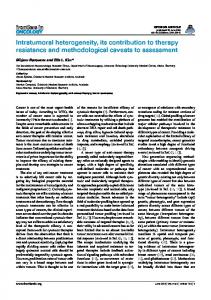
Inner nozzle Figure 1: Coaxial nozzle equipped with miniature flap actuators (Kurimoto et al. 2004).
2.0 (a)
In our previous studies (Kurimoto et al., 2004, 2005), we tried to control a coaxial methane/air jet by using miniature flap actuators arranged on the inner surface of an annular nozzle (Fig. 1) in order to achieve optimal mixing and combustion. In this method, large-scale vortex rings can be induced at the inner and outer jet shear layers perfectly in phase with the flapping motion. The size and spacing of vortices can be controlled by changing the flapping frequency as shown in Fig. 2. Large-scale vortices are shed continuously in the inner and outer shear layers when Sta (= fa Do /Um,o ) = 1.0, where fa , Do , and Um,o are the flapping frequency, the outer nozzle diameter, and the bulk mean velocity of the annular air jet, respectively. Under this
(c)
(b)
z/Do
1.5
1.0
0.5
-0.5
0.0
0.5
-0.5
0.0 r/Do
0.5
-0.5
0.0
0.5
Figure 2: Visualization of controlled jets with central jet seeded (Saiki, 2008): (a) Sta = 0.1, (b) Sta = 1.0, and (c) Sta = 1.7. 1
In order to develop even more effective control schemes for jet mixing and combustion, it is necessary to further clarify the vortex generation mechanism with the periodic forcing of different modes. In the present study, the velocity field induced by the axisymmetric flapping motion is first measured experimentally by particle imaging velocimetry (PIV) at just downstream of the nozzle exit. Then, we use the measured velocity data as inlet conditions in the numerical simulation of a coaxial jet in order to mimic the flow development precisely. Through a series of simulations, we discuss the difference in the mixing performance and the vortex generation mechanism when different excitation modes are employed. Specifically, we assess a helical mode of forcing in addition to conventional axisymmetric one.
The 6th Int. Symp. on Turbulence and Shear Flow Phenomena June. 22-24, 2009, Seoul, Korea ered rather weak from computational results with different domain sizes except for the cases when Sta > 1.2. Thus, the range of Sta in the present simulation is kept from Sta = 0.1 to 1.1. Hereafter, z, r and θ denote the streamwise, radial and azimuthal directions, respectively. The velocity ratio of Um,o /Um,i is given as 4.8 in accordance with the experiment. However, the density difference is neglected, so that 2 /ρ U 2 , results to be 23. the momentum flux ratio, ρo Um,o i m,i This difference may cause an additional influence, since it is known that the momentum flux ratio should be an important parameter for coaxial jet mixing (Rehab et al., 1997).
8Do r
Um,o
Do Di
Dw z
Um,i
EXPERIMENTAL MEASUREMENT A series of experiments (Kurimoto et al., 2004, 2005; Angele et al., 2006; Saiki, 2008) have been carried out in order to provide the fundamental knowledge on the shear layer development and also the database to verify the numerical simulation later described. The experimental setup of a coaxial jet is the same as described by Kurimoto et al. (2004). Dry air jet is issued through an annular nozzle (ID: Di = 10 mm, OD: Do = 20 mm), while methane is supplied through a central nozzle. The latter is a stainless steel tube, which is long enough to establish a fully developed laminar flow before being issued from the nozzle exit. The Reynolds number of annular jet, Um,o Do /νo , is 2.4 × 10³ , where νo is the kinematic viscosity of air. The ratios of density, ρo /ρi , bulk mean velocity, Um,o /Um,i , and momentum 2 /ρ U 2 , between the annular and central jets flux, ρo Um,o i m,i are 1.8, 4.8 and 42, respectively. In this experiment, all flap actuators are driven synchronously with a saw-tooth signal, which is found to be most effective for mixing (Kurimoto et al., 2004). After reaching the maximum displacement of 0.3 mm at φ < π, the flaps snap quickly back to the wall. The velocity field is measured with a two-component PIV. The central and annular jets are seeded with silica particles (dp = 1.2 µm, ρp = 215 kg/m3 ). A double-pulsed Nd: YAG laser (THALES, SAGA PIV20) is employed for the light source and the laser sheet is introduced into the test section. Particle images are captured by a flame-straddling CCD camera (Lavision, Flowmaster 3S). Commercial software (Lavision, Davis 7.2) is used to calculate the particle displacement in an interrogation area with a cross-correlation technique. In order to measure the velocity field induced by the flaps, a small PIV measurement region is employed just downstream of the nozzle exit. An extension tube between the camera and the objective lens is used. This arrangement allows, with 32×32 pixel interrogation windows over a measurement area of 3.33 × 2.66 mm2 , a spatial resolution of 83 µm.
θ
Figure 3: Computational domain and coordinates for LES. We solved the incompressible momentum and passive scalar transport equations with the dynamic Smagorinsky model (Germano et al., 1991) for the SGS stress and flux terms. The mean axial velocity profile is assumed to be a fully developed laminar Poiseuille flow at the central nozzle exit, while for the annular nozzle a tophat-shaped turbulent flow is given as follows:
uz (r) =
θo =
) 1 dp0 ( 2 Ri − r 2 4µ dz r − Ri Umax tanh a Ro − r Umax tanh a
−
1 2 Umax
∫
Ri +Ro 2
(
(0 ≤ r ≤ Ri )
Ri ≤ r ≤
( Ri +Ro 2
Ri +Ro 2
)
≤ r ≤ Ro
uz (r) (Umax − uz (r)) dr
) (1) (2)
Ri
The value of a in Eq. (1) determines the momentum thickness θo of the outer shear layer defined by Eq. (2). It is adjusted to represent the experimentally measured value (θo /Do = 1.5 × 10⁻² ). Random background noise is added to mimic the experimental data. GENERATION OF VORTEX RINGS IN INITIAL SHEAR LAYERS We investigated the mechanism of vortex generation near the nozzle experimentally and numerically. Figure 4(a) shows the close-up visualization images of the seeded outer jet flow at different phases of flapping motion when Sta = 0.1, whilst the corresponding radial distributions of phase-averaged radial velocity at z/Do = 0.004 are shown in Fig. 4(b). It is clearly seen that the outer shear layer is drastically deformed with the snap back motion of the flap at φ = 0.96 − 0.99π. At φ = 0.96π, strong entrainment of ambient air is identified with a large negative radial velocity, which reaches −0.15Um,o , is induced around r/Do ∼ 0.45. This is probably because static pressure near the outer shear layer becomes reduced due to the quick snapping motion (∼ 1 ms) of the flap. On the other hand, at φ = 0.99π, large positive velocity of about 0.2Um,o is found at the outer edge of nozzle exit. This induced velocity is comparable to the snapping back speed of the flap. These negative and radial velocities result in vortex ring formation within a short distance from the nozzle as shown in later. This is the primary
NUMERICAL SIMULATION A large eddy simulation (LES) code is developed based on the DNS code of Mitsuishi et al. (2007). The computational domain is shown in Fig. 3. Cylindrical coordinates are employed. Both the diameter ratio, Do /Di , and the expansion ratio, Dw /Do , equal to 2. The flow field is assumed to be surrounded by a cylindrical wall in the LES, but it is open in the experiment. However, the direct influence of this discrepancy to the initial shear layer development is consid2
reason why the saw-wave driving mode, which has the snap back motion regardless of flapping frequency, is preferable to control vortex shedding. To mimic the experimental nozzle exit condition described above, the phase-averaged radial velocity is assumed at the inlet of computational domain in the LES. The PIV data is interpolated by a polynomial function, which is 5thorder in space and first-order in time. The, fluctuating axial velocities caused by the flapping motion are given by the continuity equation at the cells located at the inlet boundary of the computational domain. (a) φ = 0.2π
The 6th Int. Symp. on Turbulence and Shear Flow Phenomena June. 22-24, 2009, Seoul, Korea Figure. 6 shows phase-averaged mixture fraction distributions and velocity vector diagrams obtained by the simulation. The successive positions computed of vortex ring formation are in good agreement with that in the experiment (Fig. 5), but the size of vortex is generally smaller, especially at the inner/outer jet interface. A plausible reason for this discrepancy should be the assumption of incompressible flow in the simulation unlike the experiment in which methane and air are employed. 1.5
φ = 0.96π
0.1
1.0
z/Do
z/Do
0.1
0.4 φ = 0.99π
0.0
0.5
(b) 0.2 0.1
z/Do
~ (v+v)/U m, o
0.1
1.5
A
0.4
0.5
ø = 0.2π ø = 0.96π ø = 0.99π
1.0 z/Do
0.0
0.5
0.0
0.5
-0.1
0.0
0.4 r/D o
-0.2 0.35
0.5
0.40 0.45 r/Do
0.50
0.0
Figure 4: Initial development of outer shear layer with Sta = 0.1: (a) visualization of annular jet, (b) radial distribution of phase-averaged radial velocity at z/Do = 0.004.
φ=π
φ = 1.07π
φ = 1.13π
f = f¯ + f˜ + f ′′
1 m/s
1.5 1 m/s
z/Do
1.0
ii' iv
ii
0.5
iii
i 0.0
0.5
0.0
0.5
0.0 r/Do
0.5
0.0
0.5
0.0
0.5
(3)
where the first, second and last terms on the right-hand sides represent mean, phase-mean, and random components, respectively. Figure 7 shows the contour lines of phase-averaged azimuthal vorticity and concentration fraction obtained by the LES with three different flapping frequencies. The concentration is also indicated as B/W gradation. It is observed that large-scale vortex rings at the inner shear layer engulf the outer annular jet fluid and entrain into the central jet. When Sta = 0.1, vortex rings are generated intermittently, and the central jet fluid near the jet axis is not much transported in the radial direction, so that the concentration fraction does not decrease immediately. As Sta is increased, both size and spacing of vortex rings become smaller and the mixing proceeds faster even around the jet axis. Figure 8 shows the radial distributions of mixture fraction statistics, i.e., the mean and the root-mean-square (rms) value of phase-mean plus random components, at different axial positions. When Sta = 0.1, the mean mixture fraction does not become uniform, whilst the rms fluctuation remains very large at z/Do = 2.0. This fact implies highly intermittent nature of the mixing process at Sta = 0.1. On the other hand, when Sta = 1.0 and 1.1, the radial entrainment
φ = 1.2π
1 m/s
0.0 r/Do
Kurimoto et al. (2004) experimentally showed that mixing concentration can be controlled by changing Sta and mixing is most enhanced when Sta = 1.0. We repeat the simulation under different Sta and confirm their conclusion below. In periodically fluctuating field, a physical variables f is decomposed as follows:
z/Do
1 m/s
0.5
CONTROL WITH DIFFERENT STROUHAL NUMBERS
1.0
0.5
0.0
Figure 6: Phase-averaged mixture fraction (upper) and velocity vectors (bottom) with Sta = 0.1 in LES.
Although the optimal flapping frequency exists around Sta = 1.0, we first execute experiment and simulation under the condition Sta = 0.1, where less interaction between vortex rings is expected because of their larger streamwise spacing. Figure 5 shows visualization images and velocity vector diagrams of the annular jet in the experiment. Negative and then positive radial velocities are induced by the flap located upstream of the outer shear layer (as indicated (i)), and negative radial velocity propagates to the inner shear layer (ii and ii’). The induced velocity eventually generates vortex rings both at the inner and outer shear layers (iii and iv). 1.5
0.5
0.5
Figure 5: Instantaneous visualization of annular jet (upper) and phase-averaged velocity vectors (bottom) with Sta = 0.1 in experiment.
3
The 6th Int. Symp. on Turbulence and Shear Flow Phenomena June. 22-24, 2009, Seoul, Korea (a) 20
2.0
(a) 4 8 -4
4
20
p(c)
5
20
10 5
20
20
Center line z/Do = 1.0 Sta 0.1 1.0 1.1
4 -8
c
0.6
15 10 5
Inner shear layer z/Do = 1.0 Sta 0.1 1.0 1.1
0 0.0 0.2 0.4
0.8 1.0
c
0.6
0.8 1.0
8
8
Figure 9: PDF of mixture fraction: (a) center line (r/Do = 0.0), (b) inner shear layer (r/Do = 0.25).
0.50
0
0.00
r/Do
12
by distributing the profile periodically with the phase shift along the azimuthal direction θ.
0.50
-16
0.00
r/Do
0
-4
-8 4 0 16 8
16
-12 -20 -16 -4 -8 0 4 16 8
0.0 0.00
16 4
-12 -16 -8 -4 0 12 8
12
16
-12
-12
0.5
0
12 16
-12
0
0
4
z/Do = 1.5
15
5
0 0.0 0.2 0.4
4 0
z/Do = 1.5
5
8
z/Do
0
10
10
-4
z/Do = 2.0
15
5
15
-4
1.0
z/Do = 2.0
10
-4
-8
20
15
-8 12
5
20 10
1.5
z/Do = 2.5
15
5 15
1.0 0.8 0.6 0.4 0.2 0.0
(c)
(b)20 10
10
c+~ c
(b)
z/Do = 2.5
15
p(c)
of scalar as well as the axial decay of fluctuation is much faster. If precisely examined, Sta = 1.0 gives the best mixing enhancement because of continuous shedding of intense vortices. Figure 9(a) and (b) show the probability density functions of mixture fraction along the center line and the inner shear layer (r/Do = 0.25), respectively. Large peaks of PDF at c ∼ 0.068 represents uniform mixing, so the change toward profiles with a peak at c ∼ 0.068 is a consequence of proceeding mixing in these figures. Again, Sta = 1.0 gives the best performance of mixing enhancement. The present results agree fairly well with the experiment of Kurimoto et al. (2004).
Figure 10(a) and (c) show instantaneous vortical structures, while Fig. 10(b) and (d) velocity vectors and mixture fraction gradation in the cross sectional plane at z/Do = 0.75. Vortical structures are visualized by the iso-surface of the second invariant of deformation tensor (II < −20). In the axisymmetric forcing mode, a vortex ring is shed from the inner shear layer ((a)-(i)), and it actively entrains central and annular jet fluids. In contrast, a spiral vortex is generated by the helical forcing ((c)-(ii)), and the resultant radial velocity, which is non-uniform in the azimuthal direction, induces characteristic entrainment of annular jet fluid. Accordingly, the mixing fraction gradation in Fig. 10(d) shows a clear spiral pattern. Figure 11 shows the radial profiles of mean and rms mixture fractions. The mean value is smaller at z/Do = 1.0 − 2.0 and the rms value is larger at z/Do = 1.0 in the helical forcing mode. This fact suggests that the radial transport of scalar is more promoted in the helical forcing mode.
0.50 r/Do
Figure 7: Contour lines of phase-averaged azimuthal vorticity (solid) and mixture fraction (dashed): (a) Sta = 0.1, (b) Sta = 1.0, (c) Sta = 1.1. z/Do = 2.0
0.2 0.1 0.4 z/Do = 1.5
2
0.2
0.2 0.0 0.0 0.2
0.1
''
z/Do = 1.0
0.4 0.3
z/Do = 1.0
0.2 0.1
0.2
0.4
z/Do = 1.5
0.3
0.4
0.6
z/Do = 2.0
0.3
0.6
1.0 0.8
(b) 0.4
~
0.25 0.20 0.15 0.10 0.05 0.30 0.25 0.20 0.15 0.10 0.05 1.0 0.8
(c+c )
c
(a) 0.30
0.4 z/Do = 0.5 Natural Sta 0.1 1.0 1.1 0.4 0.6 r/Do
0.8 1.0
0.3 0.2 0.1 0.0 0.0 0.2
z/Do = 0.5 Natural Sta 0.1 1.0 1.1
0.4 0.6 r/Do
0.8
(a)
1.0
(b)
0.0
r/Do
1.0
0.25
Figure 8: Radial distribution of mean and rms mixture fraction: (a) mean, (b) rms value.
0.5
z/Do = 0.75
(i) (c)
CONTROL WITH DIFFERENT FORCING MODES
1.0
(d)
0.0
r/Do
Entrainment of scalar by large-scale vortices We investigate how the vortical structure contributes to mixing enhancement in the axisymmetric and helical forcing modes. In each mode, the inlet radial velocity is given by: ur (r, t) = ur,exp (r, t) : Axisymmetric mode ) ( θ : Helical mode ur (r, θ, t) = ur,exp r, t + 2π
0.25
(ii)
0.5
(iii)
Figure 10: Instantaneous vortical structures (left), velocity vectors and concentraion of central jet fluid (right): (a, b) axisymmetric mode, (c, d) helical mode.
(4)
where ur,exp represents the experimentally measure velocity profiles shown in Fig. 4. The helical mode is mimicked 4
The 6th Int. Symp. on Turbulence and Shear Flow Phenomena June. 22-24, 2009, Seoul, Korea z/Do = 2.0
0.25 0.20 0.15 0.10 0.05 0.30 0.25 0.20 0.15 0.10 0.05 1.0 0.8
(b) 0.4
(a)
z/Do = 2.0
(b)
0.3
z/Do=1.0
0.2
z/Do=1.0
0.1 0.4
z/Do = 1.5
z/Do = 1.5
0.3
2
z/Do=0.75
(i)
0.2
z/Do=0.75
(i')
0.1
''
(c+c )
c
(a) 0.30
~
z/Do = 1.0
0.4 z/Do = 1.0
0.3
0.6
0.25
0.5
r/Do
0.5
0.25
r/Do
0.2
0.4
Figure 13: Streamwise vortices in near-nozzle region (a) axismmetric mode, (b) heical mode.
0.1
0.2 1.0 0.8
z/Do = 0.5 Axisymmetric Helical
0.6
0.4 0.3
z/Do = 0.5 Axisymmetric Helical
0.2
0.4
0.1
0.2 0.0 0.0 0.2
0.4 0.6 r/Do
0.8 1.0
0.0 0.0 0.2
(a) 20 0.4 0.6 r/Do
0.8
1.0
Figure 11: Radial distribution of mean and rms mixture fraction: (a) mean, (b) rms value.
z/Do = 2.5
(b)20
15
15
10
10
5
5
20
20
z/Do = 2.5
z/Do = 2.0
Mixing enhancement by streamwise vortices From the above results, it is evident that the mixing process is first enhanced by the primary ring vortex and subsequently by many streamwise vortices. Hence, we show the ensemble-averaged number of streamwise vortices at each axial position in Fig. 12. A vortex is identified by a threshold value of II = −20 and its streamwise vorticity larger than 6. The number of vortices is counted in the zone including the inner shear layer (r/Do = 0.125 − 0.375). The number of vortices first increases in the streamwise direction, but seems to be saturated later both in the PIV measurement by Angele et al. (2006) and the present numerical simulation. Although there exists a discernible difference in the two results, both show that the helical mode excitation produces more streamwise vortices. A more detailed observation of streamwise vortices induced by the two excitation modes is represented in Fig. 13. It is seen that the helical excitation generates distinct rib vortices in the braid region around z/Do ∼ 0.75 ((a)-(i) and (b)-(ii’)). Figure 14(a) and (b) show the PDF of central jet fluid concentration along the center line and the inner shear layer, respectively. The PDFs for the two forcing modes give similar distributions toward the state of uniform mixing (c ∼ 0.068) along the center line, but at the inner shear layer it is slightly larger in the helical mode excitation.
8
6
15
10
10 5
20 z/Do = 1.5
20 z/Do = 1.5
15
15
10
10
5
5
20
20
Center line z/Do = 1.0 Axisymmetric Helical
15 10
Inner shear layer z/Do = 1.0 Axisymmetric Helical
15 10
5
5
0 0.0 0.2 0.4
c
0.6
0 0.0 0.2 0.4
0.8 1.0
c
0.6
0.8 1.0
Figure 14: PDF of mixture fraction with different excitation modes: (a) center line (r/Do = 0.0), (b) inner shear layer (r/Do = 0.25).
From these results, it can be said that the helical mode excitation promotes scalar mixing much effectively than the axisymmetric excitation by generating more streamwise vortices in the inner shear layer. In addition, the vortices produced around the center line may not be much effective in mixing. As Mitsuishi et al. (2007) tried, we analyze the mechanism of streamwise vortex generation through the budget of phase-averaged streamwise enstrophy, which is given by the following equation: ∂ ∂t
4
〈
1 ′′ 2 ω 2 z
〉
〈
′′ + u′′ r ωz
2
〈
〉
1.5
+ 〈ωr 〉ψ
〈
Figure 12: Number of streamwise vortices with different excitation modes.
= −CVrψ − CVθψ − CVzψ ψ
∂ 〈ωz 〉ψ
ψ
〉 ′′
+ ωr′′ ωz
1.0 z/Do
p(c)
p(c)
5
Inner shear layer sim. exp. (Angele et al. 2006) helical axisymmetric
0 0.5
z/Do = 2.0
15
〈
+ ωz′′ ωr′′
∂r ∂ 〈uz 〉ψ
〈
〉 ψ
〉 ′′
∂ 〈ωz 〉ψ r∂θ ∂ 〈uz 〉ψ
〈
′′ + u′′ z ωz
〈
〉
〉
′′ ∂u′′ ∂u′′ 2 ∂uz z + ωz′′ ωθ′′ z + ωz′′ ∂r r∂θ ∂z
2 ωz′′ ψ
∂ 〈ωz 〉ψ
ψ
∂z ∂ 〈uz 〉ψ
+ ωθ′′ ωz + ψ ∂r r∂θ ∂z 〉 〈 〉 〈 ′′ ′′ ′′ 〉 ′′ ∂uz ′′ ∂uz ′′ ∂uz ωz + 〈ωθ 〉ψ ωz + 〈ωz 〉ψ ωz ∂r ψ r∂θ ψ ∂z ψ ψ
−T Dψ − V Dψ − DSψ 5
〈
′′ + u′′ θ ωz
〉
ψ
(5)
The first three terms on the RHS of Eq. (5) represent the convection terms in each direction. The last three terms are turbulent diffusion, viscous diffusion, and viscous dissipation, respectively. The rest of the terms are production terms. In the present simulation, each term in Eq. (5) has been calculated and it is found that the two tiling and stretching terms of production, 〈ωr′′ ωz′′ 〉ψ
〈
〉 ′′ 2
ωz
ψ
∂〈uz 〉ψ ∂z
∂〈uz 〉ψ ∂r
The 6th Int. Symp. on Turbulence and Shear Flow Phenomena June. 22-24, 2009, Seoul, Korea ACKNOWLEDGMENTS All simulations in this paper have been carried out by using HITACHI SR11000 at the Super Computing Division, Information Technology Center, The University of Tokyo. REFERENCES
,
Angele, K., Kurimoto, N., Suzuki, Y., and Kasagi, N., 2006, ”Evolution of Streamwise Vortices in a Coaxial Jet Controlled with Micro Flap Actuators”, Journal of Turbulence, Vol. 7(73), pp. 1-19. Crow, S. C. and Champagne, F. H., 1971, “ Orderly Structure in Jet Turbulence ”, Journal of Fluid Mechanics, Vol. 48, pp. 547-591. Germano, M., Piomelli, U., Moin, P. and Cabot, W. H., 1991, “ A Dynamic Subgrid-Scale Eddy Viscosity Model ”, Physics of Fluids, Vol. 3(7), pp. 1760-1765. Hilgers A., 1999, ”Parameter Optimization in Jet Flow Control”, Annual Research Briefs, Center for Turbulent Research, NASA Ames/Stanford University, pp. 179-193. Hu H., Saga T., Kobayashi T., Taniguchi N., 2002, ”Simultaneous Measurements of All Three Components of Velocity Vectors in a Lobed jet Flow by Means of Dual-Plane Stereoscopic Particle Image Velocimetry”, Physics of Fluids, Vol. 14, pp. 2128-2138. Hussain, A. K. M. F. and Zaman, K. B. M. Q., 1981, ”The ’Preferred Mode’ of the Axixymmetric Jet ”, Journal of Fluid Mechanics, Vol. 110, pp.39-71. Kurimoto, N., Suzuki, Y. and Kasagi, N., 2004, “ Active Control of Coaxial Jet Mixing with Arrayed Micro Actuators ”, Transactions of the JSME, Series B, Vol. 70, No. 694, pp. 1417-1424. Kurimoto, N., Suzuki, Y., and Kasagi, N., 2005, “ Active Control of Lifted Diffusion Flames with Arrayed Micro Actuators ”, Experiments in Fluids, Vol. 39, No. 6, pp. 995-1008. Kasagi, N., 2006, “ Toward Smart Control of Turbulent Jet Mixing and Combustion ”, JSME International Journal, Series B, Vol. 49, No. 4, pp. 941-950. Mitsuishi, A., Fukagata, K., and Kasagi, N., 2007,“NearField Development of Large-Scale Vortical Structures in a Controlled Confined Coaxial Jet ”, Journal of Turbulence, Vol. 8(23), pp. 1-27. Rehab, H., Villermaux, E. and Hopfinger, E. J., 1997, “ Flow Regimes of Large-Velocity-Ratio Coaxial Jets ”, Journal of Fluid Mechanics, Vol. 345, pp. 357-381. Saiki, Y., 2008, “ Active Control of Swirling Coaxial Jet Mixing and Combustion with Manipulation of Large-Scale Vortical Structures ”, Ph.D. dissertation, The University of Tokyo. Zaman, K. B. M. Q., Reeder, M. F. and Samimy M., 1994,“ Control of an Axisymnrnetric Jet Using Vortex Generators ”, Physics of Fluids, Vol. 6(2), pp. 778-793.
make marked contribution. Figure 15 shows
one of them, i.e., the phase-averaged distribution of the tiling terms in the plane of z/Do = 0.75, at φ = 1.8π. It is evident that the production is distributed uniformly around the jet in the case of the axisymmetric forcing, whilst it takes a spiral pattern in the helical forcing. In addition, in the braid region of the inner shear layer, the tilting effect is much more remarkable in the helical excitation than the axisymmetric one. This explains the difference in the number of streamwise vortices at the inner shear layer in Fig. 12. Note that the stretching term is smaller than the tilting term in the braid region of the inner shear layer, so that the mixing in the central region of the jet is primarily governed by the streamwise vortices produced by the tilting mechanism. (a)
300 (b)
300
0
0
0.25 0.5
0.25 0.5
r/Do
r/Do
Figure 15: Distribution of phase-averaged production term ∂〈uz 〉
of streamwise enstrophy, − 〈ωr′′ ωz′′ 〉ψ ∂r ψ , at z/Do = 0.75 and φ = 1.8π: (a) axisymmetric mode, (b) heical mode.
CONCLUSIONS We first carried out PIV measurement and flow visualization in order to explore the mechanism of initial vortex generation in the near-field of a controlled coaxial jet. The measured velocity data at the nozzle exit with the flapping excitation is used as the inlet condition for the LES simulation. It is confirmed that the simulation code can reproduce the vortex generation and mixing property in the experiment fairly well. Two different (axisymmetric and helical) forcing modes are tested and evaluated in terms of the effectiveness in mixing enhancement. Development of the primary vortices is found different between two modes, and scalar entrainment in the radial direction is more significant in the helical forcing mode. More rib vortices are generated in the inner shear layer by the helical forcing mode. This is because the tiling effect caused by the phase-averaged radial gradient of streamwise velocity is stronger in the helical mode than in the axisymmetric one. We also compared the PDFs of mixture fraction in both modes, and found that the difference of mixing enhancement between the two modes is not so large actually. However, the helical mode generates more streamwise vortices, and this suggests possibility to develop a more effective forcing mode for mixing control by selecting a different azimuthal mode for multiple distributed micro actuators. 6