MEG Adaptive Noise Suppression using Fast LMS - University of ...

Proceedings of the 2 nd International IEEE EMBS Conference on Neural Engineering Arlington, Virginia · March 16 - 19, 2005

MEG Adaptive Noise Suppression using Fast LMS Nayef E. Ahmar1, Jonathan Z. Simon1,2,3 1

Department of Electrical and Computer Engineering 2 Department of Biology 3 Bioengineering Program

University of Maryland, College Park Abstract-Magnetoencephalography (MEG) measures magnetic fields generated by electric currents in the brain, non-invasively and with millisecond temporal resolution. Typical signals are 10–13 T, so noise contamination due to external magnetic fields is a serious concern. Digital signal processing is typically required in addition to magnetic shielding. Using three reference channels, displaced from the head, to measure the noise, we apply adaptive filtering to subtract out estimates of the noise, via the Block Least-Mean-Square (“Fast LMS”) method. The algorithm is tested by its effects on the number and distribution of channels which have statistically significant signals (distinguishable from background noise at a specified false-positive rate). We show that Fast LMS both increases the number significant channels and reduces the variance of false positives.

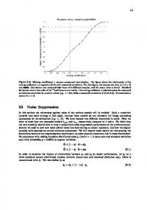
octave, 1 octave, and 5 octave pink noise all centered at 707 Hz). All stimuli were presented binaurally at approximately 70 dB SPL. 8 right handed subjects (5 female) were used and gave their written informed consent for the MEG study. The magnetic signals were recorded using a 160-channel, whole-head axial gradiometer system (KIT, Kanazawa, Japan) housed in a magnetically shielded room. Its detection coils are in a uniform array on a helmet-shaped surface of the bottom of the dewar, with ~25 mm between the centers of two adjacent 15.5 mm diameter coils. Sensors are first order axial gradiometers with 50 mm baseline; their field sensitivities are 5 fT/√Hz or better in the white noise region. 3 of the 160 channels are magnetometers (25 cm apart from neuronal data sensors), used as reference channels. The magnetic signals were band-passed between 1 Hz and 200 Hz, notch filtered at 60 Hz, and sampled at the rate of 500 Hz. Responses to each stimulus from 300 to 2300 ms poststimulus were concatenated, resulting in 20 responses (2 ms resolution, 100 s duration) for each channel. Each response was discrete Fourier Transformed (DFT), resulting in 20 complex frequency responses (0.01 Hz resolution, 250 Hz bandwidth) for each channel. See Fig. 1 for the magnitude squared of the DFT of the response (periodogram) of a single channel to the 31.5 Hz amplitude modulated sinusoid tone. The SSR peak at 31.5 Hz is stereotypically narrow with a width of 0.01 Hz. Also as seen in Fig.1, the background responses became noisier with decreasing frequency.

I. INTRODUCTION Magnetoencephalography (MEG) is a noninvasive tool that measures the magnetic activity of the brain, using extremely sensitive magnetometers based on Superconducting Quantum Interference Devices (SQUIDs). MEG has moderate spatial resolution (~ 1 cm) and extremely high temporal resolution (≤ 1 ms), thus complementing other techniques such as electroencephalography (EEG) and functional Magnetic Resonance Imaging (fMRI). Because the magnetic signals emitted by the brain are on the order of 10–13 T, shielding from external magnetic signals, including the Earth's magnetic field (~ 5x10-5 T), is necessary. Even with shielding, though, poor signal to noise ratio (SNR) is still a challenge. To remove such noise, which is typically non stationary, we resort to adaptive filtering. Three reference channels, separated from the head, measure the noise alone, while 157 neuronal channels, arranged above the head surface, record brain activity. The filter coefficients that linearly map the noise in the reference channels to the noise in the observed signal are calculated using Least Mean Square method (LMS) [13], then the estimated noise in the observed neuronal signal is subtracted. A fast version of LMS is adopted for speed [7]. To test its validity and usefulness, we use significance tests devised in [12] that combine Rayleigh’s phase coherence test and the F-test [10, 8, 11]. Comparison of the raw data with the filtered data shows substantial improvement in number of significant channels and a drop (and more consistency) in the false positives. Finally, we compare this method to the Continuously Adjusted Least-Squares Method (CALM) [5].

B. Adaptive filter model Background brain activity is always changing even if the area of interest responds to stimuli in a stationary fashion. External noise is also non-stationary since many of its sources are of random characteristics in space and time. We use an adaptive process, which automatically adjusts the filter parameters to minimize estimation error. We implement a normalized LMS method for the 3 reference channels (Fig. 2), where the adaptation of tap weight is based on error estimation. We compute the filter coefficients that when convolved with the noise signal, capture the noise in

II. METHODS A. Stimuli and Data Sinusoidally amplitude-modulated sounds of 2 s duration were presented 50 times each in a random order with interstimulus intervals uniformly distributed between 700 and 900 ms as described in [4]. A total of 20 stimuli were generated with five modulation frequencies (1.5 Hz, 3.5 Hz, 7.5 Hz 15.5 Hz and 31.5 Hz) and four different carriers (pure tone, 1/3 0-7803-8709-0/05/$20.00©2005 IEEE

v

Dimensions: r=0,…,R ; reference channels, e.g. R = 3. M; block size (e.g. 1024 samples) i=0,…,2M-1

Initialization: Wˆr (0) = zeros (2 M , R ) ; Filter coefficients initialized to zero

Pi,r (0) = δ i ; average signal power per Reference channel, initialized to small positive constant δ

.

Computation: For each block of M input samples: Filtering:

Fig. 1. (top panel) Periodogram of the Fourier transform of magnetic field response from one channel to a sinusoidal amplitude modulated tone with modulation frequency 31.5 Hz and carrier frequency 707 Hz.

U r ( k ) = diag { FFT [u r ( kM − M ),..., u r ( kM − 1), u r ( kM ),..., u r ( kM + M − 1)]T } yrT (k ) = last M elements of IFFT [U r (k )Wˆr (k )]

Error estimation: Observed signal

Error

R

e ( k ) = d ( k ) - ∑ yr ( k ) r =1

Noise Ref.#1

Noise Ref.#2

W1(Z)

⎡0 ⎤ E(k)=FFT ⎢ ⎥ ⎣ e(k) ⎦

Signal-power estimation:

W2(Z)

Pi,r (k) = γ Pi,r (k − 1) + (1 − γ ) U i,r (k) Noise Ref.#3

2

D(k) = diag[P0−1 (k), P1−1 (k),..., P2−M1 −1 (k)]

W3(Z)

Tap-weight adaptation:

Fig.2. Three reference adaptive filter noise cancellation

Φr (k) = first M elements of IFFT[D(k)U rH (k)E(k)]

⎡Φ(k ) ⎤ Wˆr (k + 1) = Wˆr (k ) + α FFT ⎢ ⎥ ⎣0 ⎦

the observed signal in a least mean square sense. With a block size of user-defined length (M), the improvement in execution time is the order of the Complexity ratio = 5log 2 M + 13 M [7]. For example, block size M = 1024, fast LMS is 16 times faster than standard LMS algorithm in computational terms. A summary of the implementation of Block LMS algorithm described in [6, 7], but modified for use with multi-reference channels is outlined in Table 1.

(

)

FFT : Fast Fourier Transform, IFFT: Inverse Fourier Transform,

α : adaptation constant