Memory Efficient Skeletonization of Utility Maps Albert M. Vossepoel1, Klamer Schutte2 and Carl F.P. Delanghe1 1 Delft
University of Technology Applied Physics, Pattern Recognition Group Lorentzweg 1, 2628 CJ Delft, The Netherlands e-mail:
[email protected] Abstract An algorithm is presented that allows to perform skeletonization of large maps with much lower memory requirements than with the straightforward approach. The maps are divided into overlapping tiles, which are skeletonized separately, using a Euclidean distance transform. The amount of overlap is controlled by the maximum expected width of any map component and the maximum size of what will be considered as a small component. Next, the skeleton parts are connected again at the middle of the overlap zones. Some examples are given for efficient memory utilization in tiling an A0 size map into a predefined number of tiles or into tiles of predefined (square) size. The algorithm is also suited for a parallel implementation of skeletonization.
2
TNO Physics and Electronics Laboratory Electro Optics Group, P.O. Box 96864 2509 JG The Hague, The Netherlands e-mail:
[email protected]
well beyond the capacity of a typical workstation, for which an A4 size drawing (45 Mbytes, including skeletonization) often presents the maximum amount of data that can be handled without having to resort to extremely decelerating virtual memory techniques. In the algorithm proposed in this paper, memory requirements are minimized by dividing the binary map in smaller rectangular and partially overlapping tiles, as shown in figure 1. The overlap of the tiles serves to allow connect the partial skeleton branches again. ∆ xM ∆x T E
∆ yT
1: Introduction ∆ yM
For many public utility organizations digital information is a primary source for design, planning and maintenance. Much of the existing information, however, is still only available in the form of maps drawn on paper, linen or similar materials. Handling the data in a geographic information system (GIS) requires more than mere digitization of these drawings into raster images: the recognition of structure and objects in the drawings, with vectorization or other decomposition methods as a prerequisite [1,2]. In the decomposition and recognition programs, however, the largest memory– and often also processing– capacities are claimed by the skeletonization procedure. A typical drawing size of 1 m 2 (A0) requires approximately 236 Mbytes of memory when scanned at 8 bits/pixel and 400 dpi, to which must be added twice this amount for a skeletonization based on the Euclidean distance transform [3]. This requirement is
Figure 1: Small part of a utility map, divided into four tiles (delineated by solid lines); the hairlines indicate the middle of the overlap zone.
2: The skeleton near a border The decomposition program ROCKI [2] for which the procedure described here is developed, is based on the perception of the (pseudo-)Euclidean skeleton as
the locus from which the connected component can be reconstructed from its pixels p using circular discs centered on p with a radius given by a distance function [4]. The problem is now to know whether or not a skeleton pixel near the tile border is a true skeleton pixel of the component, i.e., would it have been at the same location if there had been no tile border at all? A skeleton pixel of which the disk does not touch the border must be a true skeleton pixel, because its distance to the background is smaller than to the tile border. If the maximal thickness of any component in the map Dmax is known, we can be certain that skeleton pixels at a distance of Rmax = Dmax / 2 from the border will be true skeleton pixels. Rmax can be found as the maximum of the distance transform on the skeletons of all components to be processed, but that would require the whole image to be skeletonized beforehand! For that reason, the value of Rmax is an expectation, rather than a measurement, for the image at hand. To account for this uncertainty, a relative safety margin ε has to be added, so that the overlap E becomes: E > (1 + ε ) Dmax
(
{
})
E > max ((1 + ε ) ⋅ Dmax ), max( ∆xC , ∆yC )∀ C | ( AC < A0 ) ∨ (C ∈ Sc )
After skeletonization of the tile, some skeleton branches will be incomplete, corresponding with components that cross the tile borders. Furthermore, the skeleton will show aberrations near –and caused by – the tile border. The skeleton will be considered reliable from half the overlap.
3: Outline of the algorithm Before we can start processing on the binary map we have to determine the required overlap and the tile size according to the memory constraints. These application dependent parameters will be discussed in the next section. The tiles will be processed one by one and row by row. First all components in the tile are labeled. For each component the minimal and maximal coordinates are determined. In the decomposition program employed, only the large components require skeletonization. The small components, such as the dimensional symbols, are offered to an OCR (Optical Character Recognition) module. This distinction also calls for an overlap of the tiles, because the difference between small and large components is not apparent for those components that cross tile borders. To detect this distinction, the overlap E must be larger than the width ∆x C and the height ∆yC of the small components
C: E > max( ∆xC , ∆yC )∀{C | ( AC < A0 ) ∨ (C ∈ Sc )} in which AC is the area (number of pixels) of C, and A0 is a threshold value, derived from the decomposition program, and Sc is the collection of (dimensional) symbols allowed by the drawing rules. In this way a small component on the border of a tile will be fully captured within the overlap of the next tile. Combining the two conditions that apply to E, we find:
Figure 2: Same part of a utility map as in figure 1, with the four tiles (delineated by solid lines) taken apart; the hairlines again indicate the middle of the overlap zone. For that reason, we define the inner border, consisting of all pixels at a distance E / 2 from the tile border. Note that E should have an even value, in order to make the inner border pixels of two adjacent tiles exactly adjacent. An example is shown in figure 2. In the ROCKI decomposition program employed [2], branches are obtained through a topological decomposition of the skeleton, using its branch points as intersections. In order to paste two partial skeleton branches from different tiles together, new breakpoints for the skeleton branches are introduced in the decomposition. This is done by breaking up each branch connected to the tile border into a reliable and an unreliable part. The new breakpoint is formed by the inner border: the point where a skeleton branch connected to the tile border crosses the inner border is distinctly marked. Processing on the neighboring tile will yield the remainder of the branch from an (8connected) neighbor of the same marked point [5]. This is illustrated in figures 3 and 4.
however, is A0 = 1024 pixels. This implies that in this application the latter value is decisive: 1024 = 32