Memory Organization for Invariant Object ...

MEMORY ORGANIZATION FOR INVARIANT OBJECT RECOGNITION AND CATEGORIZATION

by

Guillermo Sebastián Donatti A thesis submitted in partial fulfillment of the requirements for the degree of Philosophiae Doctoris (PhD) in Neuroscience from the International Graduate School of Neuroscience Ruhr University Bochum

March 31st 2016

This research was conducted at the Institute for Neural Computation of the Ruhr University Bochum under the supervision of P.D. Dr. Rolf P. W¨ urtz

Printed with the permission of the International Graduate School of Neuroscience, Ruhr University Bochum

Statement I certify herewith that the dissertation included here was completed and written independently by me and without outside assistance. References to the work and theories of others have been cited and acknowledged completely and correctly. The “Guidelines for Good Scientific Practice” according to§ 9, Sec. 3 of the PhD regulations of the International Graduate School of Neuroscience were adhered to. This work has never been submitted in this, or a similar form, at this or any other domestic or foreign institution of higher learning as a dissertation. The abovementioned statement was made as a solemn declaration. I conscientiously believe and state it to be true and declare that it is of the same legal significance and value as if it were made under oath.

Guillermo Sebastián Donatti

Bochum, 31.03.2016

PhD Commission

Chair: Prof. Dr. Jörg T. Epplen

1st Internal Examiner: P.D. Dr. Rolf P. W¨ urtz

2nd Internal Examiner: Prof. Dr. Boris Suchan

External Examiner: Prof. Dr. Leslie S. Smith

Non-Specialist: Prof. Dr. Andreas Reiner

Date of Final Examination: 21.06.2016

Contents List of Figures . . . . . . . . . . . . . . . . . . . . . . . . . . . . . . . . . . . . . . . .

7

List of Tables . . . . . . . . . . . . . . . . . . . . . . . . . . . . . . . . . . . . . . . .

8

Abstract

12

1 Introduction

13

1.1

Outline . . . . . . . . . . . . . . . . . . . . . . . . . . . . . . . . . . . . . . . . . 17

2 Image Feature Extraction 2.1

2.2

2.3

18

Object Views . . . . . . . . . . . . . . . . . . . . . . . . . . . . . . . . . . . . . 18 2.1.1

ETH-80 Image Set . . . . . . . . . . . . . . . . . . . . . . . . . . . . . . 19

2.1.2

Columbia Object Image Library . . . . . . . . . . . . . . . . . . . . . . . 19

Object Models . . . . . . . . . . . . . . . . . . . . . . . . . . . . . . . . . . . . . 21 2.2.1

Local Image Features . . . . . . . . . . . . . . . . . . . . . . . . . . . . . 22

2.2.2

Graph Image Features . . . . . . . . . . . . . . . . . . . . . . . . . . . . 27

2.2.3

Graph Nodes Restriction . . . . . . . . . . . . . . . . . . . . . . . . . . . 28

Extraction Procedure . . . . . . . . . . . . . . . . . . . . . . . . . . . . . . . . . 29 2.3.1

Key-point Detection . . . . . . . . . . . . . . . . . . . . . . . . . . . . . 30

3 Image Feature Self-organization 3.1

3.2

Visual Dictionary . . . . . . . . . . . . . . . . . . . . . . . . . . . . . . . . . . . 35 3.1.1

Feature Distribution . . . . . . . . . . . . . . . . . . . . . . . . . . . . . 36

3.1.2

Feature Similarity . . . . . . . . . . . . . . . . . . . . . . . . . . . . . . . 36

Growing Neural Gases . . . . . . . . . . . . . . . . . . . . . . . . . . . . . . . . 39 3.2.1

3.3

3.4

34

Bootstrapping . . . . . . . . . . . . . . . . . . . . . . . . . . . . . . . . . 44

Neural Map . . . . . . . . . . . . . . . . . . . . . . . . . . . . . . . . . . . . . . 45 3.3.1

Self-organized Topology . . . . . . . . . . . . . . . . . . . . . . . . . . . 45

3.3.2

Intelligent Feature Matching . . . . . . . . . . . . . . . . . . . . . . . . . 47

Neural Map Hierarchy . . . . . . . . . . . . . . . . . . . . . . . . . . . . . . . . 47 3.4.1

Taxonomy-based Memory Modeling . . . . . . . . . . . . . . . . . . . . . 49 4

CONTENTS

3.4.2 3.5

Coarse to Fine Feature Matching . . . . . . . . . . . . . . . . . . . . . . 49

Semantic Correlation Graph . . . . . . . . . . . . . . . . . . . . . . . . . . . . . 51 3.5.1

Image Feature Cross-correlation . . . . . . . . . . . . . . . . . . . . . . . 51

3.5.2

Co-occurrence of Image Features . . . . . . . . . . . . . . . . . . . . . . 54

4 Image Feature Clustering 4.1

56

Enhanced Tree Growing Neural Gas . . . . . . . . . . . . . . . . . . . . . . . . . 57 4.1.1

Identifying Changes in the Growing Neural Gas Network . . . . . . . . . 57

4.1.2

Adaptation of the Tree Hierarchy . . . . . . . . . . . . . . . . . . . . . . 58

4.1.3

Enhanced Tree Growing Neural Gas Algorithm . . . . . . . . . . . . . . 60

4.1.4

Growing Neural Gas Labeling . . . . . . . . . . . . . . . . . . . . . . . . 61

4.2

Data Quantization . . . . . . . . . . . . . . . . . . . . . . . . . . . . . . . . . . 62

4.3

Dimensionality Reduction . . . . . . . . . . . . . . . . . . . . . . . . . . . . . . 63

4.4

4.3.1

Principal Component Analysis . . . . . . . . . . . . . . . . . . . . . . . . 64

4.3.2

Modified Locally Linear Embedding . . . . . . . . . . . . . . . . . . . . . 67

Natural Clusters in Texture Information . . . . . . . . . . . . . . . . . . . . . . 70 4.4.1

Validation Criteria . . . . . . . . . . . . . . . . . . . . . . . . . . . . . . 72

5 Object Recognition and Categorization 5.1

5.2

76

Experimental Set-up . . . . . . . . . . . . . . . . . . . . . . . . . . . . . . . . . 77 5.1.1

Data Preprocessing . . . . . . . . . . . . . . . . . . . . . . . . . . . . . . 77

5.1.2

Data Partitioning . . . . . . . . . . . . . . . . . . . . . . . . . . . . . . . 77

5.1.3

Model Evaluation . . . . . . . . . . . . . . . . . . . . . . . . . . . . . . . 79

Feature Granularity . . . . . . . . . . . . . . . . . . . . . . . . . . . . . . . . . . 80 5.2.1

Empirically Determined Neural Plasticity . . . . . . . . . . . . . . . . . . 82

5.3

Bootstrapping . . . . . . . . . . . . . . . . . . . . . . . . . . . . . . . . . . . . . 83

5.4

Optimization of Growing Neural Gas Parameters . . . . . . . . . . . . . . . . . 85 5.4.1

Optimizing Parameter Values . . . . . . . . . . . . . . . . . . . . . . . . 85

5.4.2

Selecting the Fittest Individuals for Cross-validation . . . . . . . . . . . . 89

5.4.3

Cross-validating the Evolutionary Optimization Scheme . . . . . . . . . . 93

5.5

Local Feature Selection . . . . . . . . . . . . . . . . . . . . . . . . . . . . . . . . 97

5.6

Key-point Detection . . . . . . . . . . . . . . . . . . . . . . . . . . . . . . . . . 98

5.7

Data Quantization and Dimensionality Reduction . . . . . . . . . . . . . . . . . 100

5.8

Cross-comparison . . . . . . . . . . . . . . . . . . . . . . . . . . . . . . . . . . . 103 5.8.1

Invariant Object Recognition . . . . . . . . . . . . . . . . . . . . . . . . 103

5.8.2

Novel Object Categorization . . . . . . . . . . . . . . . . . . . . . . . . . 106

5

CONTENTS

6 Discussion

111

6.1

Texture-Based Representations . . . . . . . . . . . . . . . . . . . . . . . . . . . 111

6.2

Extraction Landmarks . . . . . . . . . . . . . . . . . . . . . . . . . . . . . . . . 112

6.3

Neural Network Bootstrapping . . . . . . . . . . . . . . . . . . . . . . . . . . . . 113

6.4

Evolutionary Optimization of Parameter Values . . . . . . . . . . . . . . . . . . 113

6.5

Emergence of Natural Clusters . . . . . . . . . . . . . . . . . . . . . . . . . . . . 115

6.6

Artificial Systems: State of the Art . . . . . . . . . . . . . . . . . . . . . . . . . 117 6.6.1

General Remarks . . . . . . . . . . . . . . . . . . . . . . . . . . . . . . . 121

7 Conclusion and Further Research

122

References

125

Appendices

136

A Implementation Details

137

A.1 Hardware Specifications . . . . . . . . . . . . . . . . . . . . . . . . . . . . . . . 137 A.2 Software Libraries . . . . . . . . . . . . . . . . . . . . . . . . . . . . . . . . . . . 137 B Supplementary Results

139

Curriculum Vitae

158

Previously Published Contents

161

Acknowledgments

162

6

List of Figures 1.1

Examples of artificial systems found in literature. . . . . . . . . . . . . . . . . . 16

2.1

Samples of the ETH-80 image set. . . . . . . . . . . . . . . . . . . . . . . . . . . 20

2.2

Samples of the COIL-100. . . . . . . . . . . . . . . . . . . . . . . . . . . . . . . 21

2.3

Example of Gabor filters. . . . . . . . . . . . . . . . . . . . . . . . . . . . . . . . 24

2.4

Families of frequency kernels. . . . . . . . . . . . . . . . . . . . . . . . . . . . . 25

2.5

Graph image feature representation. . . . . . . . . . . . . . . . . . . . . . . . . . 28

2.6

Local image feature extraction. . . . . . . . . . . . . . . . . . . . . . . . . . . . 29

2.7

Graph image feature extraction. . . . . . . . . . . . . . . . . . . . . . . . . . . . 30

3.1

Example of the Growing Neural Gas algorithm. . . . . . . . . . . . . . . . . . . 40

3.2

Example of the Growing Neural Gas Bootstrapping algorithm. . . . . . . . . . . 46

3.3

Example of a taxonomic hierarchy. . . . . . . . . . . . . . . . . . . . . . . . . . 48

3.4

Object taxonomy of the ETH-80 image set. . . . . . . . . . . . . . . . . . . . . . 50

4.1

Adaptation of the tree hierarchy when a cluster in the GNG network splits up. . 59

4.2

Adaptation of the tree hierarchy when two clusters in the GNG network merge.

4.3

Example of the Principal Component Analysis.

4.4

Conceptual overview of the Locally Linear Embedding algorithm. . . . . . . . . 67

4.5

Scree test results. . . . . . . . . . . . . . . . . . . . . . . . . . . . . . . . . . . . 71

5.1

The summary of the evolutionary optimization process. . . . . . . . . . . . . . . 90

5.2

Samples of ETH-80 object views used for the training and testing procedures. . 91

5.3

The mean errors’ components of the GNG networks observed during the epochs

60

. . . . . . . . . . . . . . . . . . 65

of the training procedure. . . . . . . . . . . . . . . . . . . . . . . . . . . . . . . 92 5.4

Histograms of the Significance Criterion. . . . . . . . . . . . . . . . . . . . . . . 101

5.5

Histograms of the Fisher’s discriminant ratio. . . . . . . . . . . . . . . . . . . . 102

6.1

The difference between the nearest and the farthest neighbors in the approximated manifold. . . . . . . . . . . . . . . . . . . . . . . . . . . . . . . . . . . . . 117 7

List of Tables 4.1

Feature Clustering. The topologies of the neural networks resulting from the Enhanced Tree Growing Neural Gas algorithm. . . . . . . . . . . . . . . . . . . 72

4.2

Feature Clustering. Analysis of the clusters resulting from the Enhanced Tree Growing Neural Gas algorithm. . . . . . . . . . . . . . . . . . . . . . . . . . . . 73

4.3

Feature Clustering. External validation criteria of the clusters obtained with the Enhanced Tree Growing Neural Gas algorithm. . . . . . . . . . . . . . . . . . . 75

5.1

Feature Granularity. General object categorization percentages for the leaveone-out cross-validation. . . . . . . . . . . . . . . . . . . . . . . . . . . . . . . . 82

5.2

Feature Granularity. General invariant object recognition percentages for the incremental hold-out validation. . . . . . . . . . . . . . . . . . . . . . . . . . . . 83

5.3

Feature granularity. Averaged Neural Map topologies for the incremental holdout validation. . . . . . . . . . . . . . . . . . . . . . . . . . . . . . . . . . . . . . 84

5.4

Bootstrapping. General object categorization percentages for the leave-one-out cross-validation. . . . . . . . . . . . . . . . . . . . . . . . . . . . . . . . . . . . . 85

5.5

The GNG algorithm parameters comprised by the individuals. . . . . . . . . . . 86

5.6

Genome of the selected fittest individuals for each evaluated approach. . . . . . 93

5.7

Optimization Through Evolutionary Algorithms. Neural Map growth and bootstrapping limits of the invariant object recognition experiments. . . . . . . . . . 94

5.8

Optimization Through Evolutionary Algorithms. General invariant object recognition percentages for the incremental hold-out validation. . . . . . . . . . . . . 95

5.9

Optimization Through Evolutionary Algorithms. Averaged Neural Map topologies for the incremental hold-out validation. . . . . . . . . . . . . . . . . . . . . 96

5.10 Optimization Through Evolutionary Algorithms. General object categorization percentages for the leave-one-out cross-validation. . . . . . . . . . . . . . . . . . 97 5.11 Local Feature Selection. General object categorization percentages for the leaveone-out cross-validation. . . . . . . . . . . . . . . . . . . . . . . . . . . . . . . . 98 5.12 Key-point Detection. Neural growth and bootstrapping limits. . . . . . . . . . . 99

8

LIST OF TABLES

5.13 Key-point Detection. General object categorization percentages for the leaveone-out cross-validation. . . . . . . . . . . . . . . . . . . . . . . . . . . . . . . . 100 5.14 Data Quantization and Dimensionality Reduction. General object categorization percentages for the leave-one-out cross-validation. . . . . . . . . . . . . . . . . . 101 5.15 Neural Map growth and bootstrapping limits of the invariant object recognition experiments. . . . . . . . . . . . . . . . . . . . . . . . . . . . . . . . . . . . . . . 104 5.16 Cross-Comparison. General invariant object recognition percentages for the incremental hold-out validation of the ETH-80 image set. . . . . . . . . . . . . . . 105 5.17 Cross-comparison. Incremental hold-out validation of the ETH-80 image set’s basic level categories. . . . . . . . . . . . . . . . . . . . . . . . . . . . . . . . . . 106 5.18 Cross-comparison. Incremental hold-out validation of the COIL-100. . . . . . . . 107 5.19 Cross-comparison. Averaged Neural Map topologies obtained using SDE/Emp parametrization for the incremental hold-out validation of ETH-80 object views. 108 5.20 Cross-comparison. Averaged Neural Map topologies obtained using the SDE/Emp parametrization for the incremental hold-out validation of COIL-100 object views.109 5.21 Cross-comparison. General object categorization percentages for the leave-oneout cross-validation.

. . . . . . . . . . . . . . . . . . . . . . . . . . . . . . . . . 109

5.22 Cross-comparison. Detailed object categorization percentages for the leave-oneout cross-validation.

. . . . . . . . . . . . . . . . . . . . . . . . . . . . . . . . . 110

B.1 Feature Granularity. Detailed object categorization percentages for the leaveone-out cross-validation. . . . . . . . . . . . . . . . . . . . . . . . . . . . . . . . 139 B.2 Feature Granularity. Detailed invariant object recognition percentages for the incremental hold-out validation with 90% of the view points used during learning and 10% on recall. . . . . . . . . . . . . . . . . . . . . . . . . . . . . . . . . . . 140 B.3 Feature Granularity. Detailed invariant object recognition percentages for the incremental hold-out validation with 70% of the view points used during learning and 30% on recall. . . . . . . . . . . . . . . . . . . . . . . . . . . . . . . . . . . 140 B.4 Feature Granularity. Detailed invariant object recognition percentages for the incremental hold-out validation with 50% of the view points used during learning and 50% on recall. . . . . . . . . . . . . . . . . . . . . . . . . . . . . . . . . . . 141 B.5 Feature Granularity. Detailed invariant object recognition percentages for the incremental hold-out validation with 30% of the view points used during learning and 70% on recall. . . . . . . . . . . . . . . . . . . . . . . . . . . . . . . . . . . 141 B.6 Feature Granularity. Detailed invariant object recognition percentages for the incremental hold-out validation with 10% of the view points used during learning and 90% on recall. . . . . . . . . . . . . . . . . . . . . . . . . . . . . . . . . . . 142 9

LIST OF TABLES

B.7 Bootstrapping. Detailed object categorization percentages for the leave-one-out cross-validation. . . . . . . . . . . . . . . . . . . . . . . . . . . . . . . . . . . . . 142 B.8 Optimization Through Evolutionary Algorithms. Detailed invariant object recognition percentages for the incremental hold-out validation with 90% of the view points used during learning and 10% on recall. . . . . . . . . . . . . . . . . . . . 143 B.9 Optimization Through Evolutionary Algorithms. Detailed invariant object recognition percentages for the incremental hold-out validation with 70% of the view points used during learning and 30% on recall. . . . . . . . . . . . . . . . . . . . 144 B.10 Optimization Through Evolutionary Algorithms. Detailed invariant object recognition percentages for the incremental hold-out validation with 50% of the view points used during learning and 50% on recall. . . . . . . . . . . . . . . . . . . . 145 B.11 Optimization Through Evolutionary Algorithms. Detailed invariant object recognition percentages for the incremental hold-out validation with 30% of the view points used during learning and 70% on recall. . . . . . . . . . . . . . . . . . . . 146 B.12 Optimization Through Evolutionary Algorithms. Detailed invariant object recognition percentages for the incremental hold-out validation with 10% of the view points used during learning and 90% on recall. . . . . . . . . . . . . . . . . . . . 147 B.13 Optimization Through Evolutionary Algorithms. Detailed object categorization percentages for the leave-one-out cross-validation. The neural growth of Neural Map Classifiers (NMC) is limited to 0.25% (L2) of their training data sets cardinality. . . . . . . . . . . . . . . . . . . . . . . . . . . . . . . . . . . . . . . . 148 B.14 Optimization Through Evolutionary Algorithms. Detailed object categorization percentages for the leave-one-out cross-validation. The neural growth of Neural Map Classifiers (NMC) is limited to 0.1% (L1) of their training data sets cardinality.149 B.15 Optimization Through Evolutionary Algorithms. Detailed object categorization percentages for the leave-one-out cross-validation. The neural growth of Neural Map Classifiers (NMC) is limited to 0.05% (L 12 ) of their training data sets cardinality. . . . . . . . . . . . . . . . . . . . . . . . . . . . . . . . . . . . . . . . 150 B.16 Key-point Detection. Detailed object categorization percentages for the leaveone-out cross-validation. . . . . . . . . . . . . . . . . . . . . . . . . . . . . . . . 151 B.17 Local Feature Selection. Detailed object categorization percentages for the leaveone-out cross-validation. . . . . . . . . . . . . . . . . . . . . . . . . . . . . . . . 152 B.18 Data Quantization and Dimensionality Reduction. Detailed object categorization percentages for the leave-one-out cross-validation. . . . . . . . . . . . . . . 152 B.19 Neural Map Hierarchy. Detailed invariant object recognition percentages for the incremental hold-out validation of the ETH-80 image set. . . . . . . . . . . . . . 153 10

LIST OF TABLES

B.20 Semantic Correlation Graph. Detailed invariant object recognition percentages for the incremental hold-out validation of the ETH-80 image set with 90% of the view points used during learning and 10% on recall. . . . . . . . . . . . . . . . . 154 B.21 Semantic Correlation Graph. Detailed invariant object recognition percentages for the incremental hold-out validation of the ETH-80 image set with 70% of the view points used during learning and 30% on recall. . . . . . . . . . . . . . . . . 154 B.22 Semantic Correlation Graph. Detailed invariant object recognition percentages for the incremental hold-out validation of the ETH-80 image set with 50% of the view points used during learning and 50% on recall. . . . . . . . . . . . . . . . . 155 B.23 Semantic Correlation Graph. Detailed invariant object recognition percentages for the incremental hold-out validation of the ETH-80 image set with 30% of the view points used during learning and 70% on recall. . . . . . . . . . . . . . . . . 155 B.24 Semantic Correlation Graph. Detailed invariant object recognition percentages for the incremental hold-out validation of the ETH-80 image set with 10% of the view points used during learning and 90% on recall. . . . . . . . . . . . . . . . . 156 B.25 Neural Map Hierarchy. General object categorization percentages for the leaveone-out cross-validation of the ETH-80 image set. . . . . . . . . . . . . . . . . . 156 B.26 Neural Map Hierarchy. Detailed object categorization percentages for the leaveone-out cross-validation of the ETH-80 image set. . . . . . . . . . . . . . . . . . 157

11

Abstract Using distributed representations of objects enables artificial systems to be more versatile regarding inter- and intra-category variability, improving the appearance-based modeling of visual object understanding. They are built on the hypothesis that object models are structured dynamically using relatively invariant patches of information arranged in visual dictionaries, which can be shared across objects from the same category. However, implementing distributed representations efficiently to support the complexity of invariant object recognition and categorization remains a research problem of outstanding significance for the biological, the psychological, and the computational approach to understanding visual perception. The present work focuses on solutions driven by top-down object knowledge. It is motivated by the idea that, equipped with sensors and processing mechanisms from the neural pathways serving visual perception, biological systems are able to define efficient measures of similarities between properties observed in objects and use these relationships to form natural clusters of object parts that share equivalent ones. Based on the comparison of stimulus-response signatures from these object-tomemory mappings, biological systems are able to identify objects and their kinds. The present work combines biologically inspired mathematical models to develop memory frameworks for artificial systems, where these invariant patches are represented with regular-shaped graphs, whose nodes are labeled with elementary features that capture texture information from object images. It also applies unsupervised clustering techniques to these graph image features to corroborate the existence of natural clusters within their data distribution and determine their composition. The properties of such computational theory include self-organization and intelligent matching of these graph image features based on the similarity and co-occurrence of their captured texture information. The performance to model invariant object recognition and categorization of feature-based artificial systems equipped with each of the developed memory frameworks is validated applying standard methodologies to well-known image libraries found in literature. Additionally, these artificial systems are cross-compared with state-of-the-art alternative solutions. In conclusion, the findings of the present work convey implications for strategies and experimental paradigms to analyze human object memory as well as technical applications for robotics and computer vision.

12

Chapter 1 Introduction One fundamental aspect of perception is the processing of visual information and its relation to the accumulated world knowledge. Many everyday life activities require identifying which objects are present in a natural scene and inferring their properties from their physical appearance. These requirements can be subsumed under the processes of object recognition, which refers to a decision about an object’s unique identity, and object categorization that states the object’s kind [92]. The fact that humans and most mammals can establish the equivalence of objects in a natural scene with the ones previously seen almost instantly and effortlessly, belies the computational challenges of modeling invariant object recognition and categorization. Developing hypotheses for the brain mechanisms that underlie visual object understanding [68] and validating them with artificial systems is a research labor of outstanding significance for the biological, the psychological, and the computational approach to comprehend perception. The complexity of modeling these tasks comes from the fact that the space of all possible views of all objects to be recognized or categorized is prohibitively large, which results in high disparity between the known and the newly encountered object perceptions. This variability can be grounded by the fact that objects in natural scenes are observed from different viewing positions, defined by the direction and distance relative to their observer. Additionally, the objects’ shape can vary considerably in both inter- and intra-category. Objects in natural scenes are usually not isolated but normally seen against different backgrounds, interacting with more objects, and sometimes partially occluded by some of them. Furthermore, objects are subjected to photometric effects including the position and distribution of light sources in the scene, their wavelengths, the effects of mutual illumination with other objects, and the distribution of shadows and specularities [86]. Each one of these transformations applied to an already seen object generates a different view, characterized with the particular frame of reference given by the object’s viewing conditions. Studied artificial or biological systems are unable to retain, or even to be aware of, all existing object views. Instead, they generalize the ones that are 13

CHAPTER 1. INTRODUCTION

perceived through a learning process that develops and continuously refines internal visual representations, denominated models, of their comprised objects. Visual object understanding relies on the comparison of recently perceived and already acquired object models, either to discriminate among physically similar ones in the case of recognition, or to generalize common properties across physically different ones during categorization. Defining the nature of the information contained in these visual representations as well as discerning the mechanisms of their associated learning process have been the source of fruitful labor for many scientists. Theories of object modeling originated with the idea that objects can be represented by relationships of a small set of LEGO-like blocks with simple geometric shapes, typically convex and volumetric, commonly known as Geons [9]. Models using this kind of representation are referred to as part-based and they generally do not contain color, brightness, texture, or depth information. Alternatively, they use polytopes like cylinders, blocks, wedges, and cones to describe object components and capture the mapping from two-dimensional space relations to infer three-dimensional shapes (e.g., a house can be modeled with a pyramid on top of a cube). Partbased object models are appealing due to their view-point and illumination invariance as well as their robustness to partial occlusion and degradation by visual noise. Nevertheless, there is not enough neurophysiological evidence to support the explicit encoding of spatial relation [91]. Moreover, several psychophysical studies [12, 84] suggest that the differences between familiar and unfamiliar object views have an impact on object recognition performance and dispute the relevance of Geon-like structural descriptions for object categorization. These arguments favor the idea that the human visual system uses appearance-based object models, constituted by measurable properties [83] (e.g., shape, illumination, shade, color, texture, or combinations), so-called image features, which are derived from a collection of two-dimensional object views. Appearance-based models are able to preserve the richness observed in a two-dimensional image because of the capability of their image features to encode diverse information available in object-views, but in detriment of their representational invariance. There are different computational approaches to object recognition and categorization using appearance-based object models. They often variate on the level of abstraction and the type of information they capture from object views, as well as in the underlying mechanisms they employ to learn and recall object models. In most cases, artificial systems have either a featuredbased [23, 24, 31, 73, 74, 79, 80] or a correspondence-based [37, 50, 89, 96, 97, 101] approach. In both cases, the processing of an object view relies on the extraction of image features together with the use of stored object models derived from previously seen object views. The first ones focus on detecting which features are present, or absent, in the object view in order to make a decision about its identity or to identify its kind. These models frequently fail when they are confronted with realistic images of natural scenes, which have complex backgrounds, multiple 14


objects, or occlusion. The latter ones store object models as ordered arrays of local features which are matched with object views by solving the correspondence problem1 ; although those models perform better on realistic images, they usually encounter problems when they are applied to large repertoires of objects where the derived object models are too complex to be generalized. Traditional artificial systems using feature- or correspondence-based approaches found in literature are exemplified in Figure 1. Some of the invariance limitations of appearance-based object models can be partially solved using image features that apply transformations of size, translation, and picture-plane rotation to already seen object views, and use their resulting values to understand novel ones. However, variations in depth-plane rotation, illumination, or shape are too complex to be compensated without considerably incrementing the amount of object models required to cover these changes, which predominantly renders their approaches for invariant object recognition and categorization computationally intractable. Having more distributed visual representations of objects enables artificial systems to be more versatile to their inter- and intra-category variability. Current research trends go towards the development of artificial systems that use appearancebased object models, like the one introduced by Westphal and W¨ urtz [95], which combine feature- and correspondence-based approaches. This combined approach is built on the hypothesis that object models are structured dynamically using relatively invariant patches of information, which can be shared across objects from the same category. These patches are represented with regular-shaped graphs, termed parquet graphs, whose nodes are labeled with elementary features that capture texture information from the object view. Their proposed graph dynamics use a two-stage procedure for object recognition and categorization. First, a feature-based approach limits the set of object candidates and their observed parquet graphs are bind together to generate model candidates. Second, these ambiguous cases are subjected to a correspondence-based approach to reach a final decision about the object identity or category. Object recognition experiments from Westphal and W¨ urtz [95] report favorable results when compared to purely feature- or correspondence-based approaches [65, 93], notably for the more sophisticated recognition tasks, such as images with structured background, multiple objects, or partially occluded objects. In contra-position, the results of experimental work [94] using this artificial system on object categorization as well as on the estimation of pose and illumination type of human faces as a categorization task, does not achieve a similar degree of success, and performs beneath feature-based artificial systems [53] when confronted with inter-category variability. 1

The correspondence problem deals with finding an organized set of point-to-point correspondences between

points in the object view and the object model.

15


Aspect representation of a Tom Cat figure View-tuned cells

Complex composite cells (C2)

Composite feature cells (S2)

Complex cells (C1)

Simple cells (S1)

weighted sum MAX

neighbor samples on the viewsphere

(a)

(b) Bunch of Jets

Gabor Wavelet Jet

Bunch Graph

Model of frontal-pose Human heads

(c)

Figure 1.1: Examples of artificial systems found in literature. (a) the object recognition in cortex [73] inspired in the primate visual cortex, further extensions [74, 80], and other systems like the Neocognitron [31], use a sequence of feed-forward neural representations based on the simple to complex hierarchy found by Hubel and Wiesel [43]. (b) the View Manifolds [96] generates a two dimensional mapping of all the possible object views from a three dimensional view-sphere and relates them according to their similarity. (c) Elastic Bunch Graph Matching (EBGM) [97], a further extension of Elastic Graph Matching (EGM) [50], which relies on the idea that objects within one class share the same landmarks with approximately identical geometrical relations. EBGM allows for the representation of a whole class of objects with a single object model using two dimensional graphs whose nodes are labeled with high-dimensional local image features described by complex responses of a set of Gabor filters [16, 32, 46] known as Gabor jets [11].

16


1.1

Outline

Using distributed visual representations, like the one proposed by Westphal and W¨ urtz [95], is a step forward to overcome invariance limitations of appearance-based object models. The accumulated world knowledge from artificial systems in-line with this computational approach is no longer a set of object models, instead, it comprehends collections of reusable object parts arranged in a visual dictionary. Moving further in this line of research requires developing mechanisms to improve the information quantization and retrieval of these dictionaries. But how can such mechanisms be developed? The present work suggests that, equipped with sensors and processing mechanisms from the neural pathway serving conscious visual perception [4], biological systems are able to define efficient measures of similarities between properties observed in objects, and use these relationships to form natural clusters of object parts that share equivalent ones. Based on the comparison of stimulus-response signatures from these object-to-memory mappings, biological systems are able to understand objects’ identities and kinds. This hypothesis focuses on the top-down aspects of visual perception and its validation brings more insight into studies of memory formation and retrieval. The starting point for the development of a computational theory to validate this hypothesis is to specify how its related artificial systems perceive the world. Consequently, Chapter 2 describes image sets, which contain segmented images of object-views from a variety of object categories. It also details the mathematical definitions behind local image features, which measure properties of objects, the mechanisms used to extract them from the object-view, and alternative types of graph image features, such as parquet graphs, which specify object parts with different levels of granularity. Combining biologically inspired mathematical models, Chapter 3 introduces three approaches to develop a memory organization framework for the graph image features available in visual dictionaries. Each of these approaches establishes its own criteria to build relationships of equivalence between the graph image features. In Chapter 5, these approaches are embedded into feature-based artificial systems to measure the information quantization and retrieval capabilities of their resulting object-to-memory mappings during invariant object recognition and categorization. In addition, the present work applies unsupervised clustering techniques to graph image features to corroborate the existence of natural clusters within their feature distribution and determine their composition. Chapter 4 describes these clustering experiments and the feasibility to use their resulting schemes to develop a hierarchical memory framework. To conclude, Chapter 6 analyses the results of this computational theory, and Chapter 7 summarizes its contribution to Neuroscience and postulates further steps in this line of research.

17

Chapter 2 Image Feature Extraction The nature of the visual object knowledge representations introduced in Chapter 3 is driven by the statistical properties of texture-based data distributions. These underlying characteristics from the observable world are unable to be generalized and they can only be approximated through a sampling procedure based on a limited set of images. This sampling procedure is denominated image feature extraction. It uses over-complete methods to derive measurable object information, so-called features, from the images outlined in Section 2.1. Section 2.2 describes how these methods model the behavior of simple and complex cells from primary visual cortex [4], to generate compositional representations of objects with the derived image features. Section 2.3 outlines the computational theory behind such biologically inspired methods. Its implementation details determine what type of information is extracted from the images and how it is structured to be further processed by the artificial systems presented in Chapter 5 in order to accomplish object recognition and categorization.

2.1

Object Views

The visual stimuli used in the present work is given by snapshots of single objects in a controlled environment. Each of these object views results from the combination of an unsegmented image of the object and its corresponding segmentation mask. The object images are taken under predefined view-point, photometric, and setting conditions using a simple background to minimize occlusion and specularity. The segmentation masks provide the locations of the pixel areas in the object image that belong exclusively to the object. This location information is also referred to as ground truth and it is used in the object views to replace the original background with a uniform color.

18

CHAPTER 2. IMAGE FEATURE EXTRACTION

2.1.1

ETH-80 Image Set

The ETH-80 image set [53] is motivated by cognitive psychology studies about how humans organize knowledge at different levels. This is a subset of the COGVIS1 database particularly designed to serve as the basis for both psychophysical and computational studies concerning object categorization. It contains views and segmentation masks of 80 objects within a taxonomy composed of 8 basic level categories (i.e., cows, dogs, horses, apples, pears, tomatoes, cars, and cups) from 4 superordinate areas (i.e., animals, fruits and vegetables, human made big, and human made small). Each category contains 10 different individuals. Every one of these objects is represented by 41 images from view-points spaced equally over the upper viewing hemisphere at distances of 22.5 – 26, which result from subdividing the faces of an octahedron to the third recursion level. The original images of this set are colored, cropped to contain a centered object plus a 20% border area, and with a resolution ranging from 400 × 400 to 700 × 700 pixels depending on the

object’s size. The standard version of these images are rescaled to a size of 256 × 256 pixels.

A close version of these images are gray value, rescaled to 128 × 128 pixels, and modified to

contain only the object without any border area. In line with the object data base described in Section 2.1.2, the ETH-80 image set also provides a close-perimg version, where each image is rescaled to 128 × 128 pixels ensuring that the object’s bounding box always fills the complete canvas size. Furthermore, this image set contains a contour version of these images, which depicts the objects’ silhouette in their original resolution. Object categorization and view-point invariant recognition experiments described in Chapter 5, as well as clustering experiments introduced in Chapter 4, employ a modified version of the close-perimg that combines the object views and their respective segmentation masks to generate segmented images. Examples from these images are depicted in Figure 2.1.1.

2.1.2

Columbia Object Image Library

The Columbia Object Image Library [66] (COIL) is designed for object recognition experiments and is widely used in literature to benchmark artificial visual systems [37]. It contains 7200 segmented views from 100 objects with a wide variety of complex geometric and reflectance properties. In comparison with the ETH-80 image set, these objects are not arranged in a deep taxonomy, instead only their identities are provided as ground truth. The COIL-100 data base comprehends colored images generated within the object’s upper viewing hemisphere with a fixed vertical angle of 75◦ and rotating 360◦ horizontally by steps 1

The COGVIS project seeks to construct a common database that may be used in psychophysical and

computational studies of object recognition and categorization.

19


Figure 2.1: ETH-80 object views. Samples from the close-perimg image set extracted from a vertical angle of 90◦ and a horizontal angle of 68◦ . In this case, the object images are combined with their segmentation masks resulting in segmented colored images scaled to 128 × 128 pixels, which contain only one object without any border area.

of 5◦ . Each image captures an object view clipped with a rectangular bounding box; then it is resized to 128×128 pixels, keeping the aspect-ratio and using interpolation decimation filters to minimize aliasing; and finally its brightness is scaled in the unsigned 16 bit range. The authors of this library also provide a gray valued image data base, denominated COIL-20, which is generated from a subset of the original objects with similar characteristics. The present work uses the COIL-100 in view-point invariant object recognition experiments detailed in Chapter 5; examples of these objects are depicted in Figure 2.1.2.

20


Figure 2.2: COIL-100 object views. Samples from the Columbia Object Image Library (COIL) extracted from a vertical angle of 75◦ and a horizontal angle of 65◦ . This library provides images scaled to 128 × 128 pixels. The object in the image is already segmented with a black

colored background.

2.2

Object Models

The use of model graphs derived from training object views are successfully applied in face detection, categorization, and recognition systems [37]. In this particular case, a person’s identity is model using a face graph [49], which has a fixed topology based on the facial landmarks configuration. This modeling approach is further generalized to multiple person identities by combining one or more face graphs with the same topology into a bunch graph [97]. The use of such general face knowledge representations are more robust to variations in the facial image, at the expense of incrementing the computational time and memory requirements linearly with the amount of combined face graphs. Usual visual scenes contain diverse types of objects. In this more abstract case, the variabil21


ity of object views generated by image transformations (i.e., view-point, background, and shape variations; photometric effects; and occlusion) considerably overcomes the one found in faces and, consequently, their landmarks become hard to determine. This challenge is dealt by using models either characterized with a grid graph [3, 50] or a dynamically assembled graph [95]. While the topology of the former follows predefined nodes, distributed equidistantly in the object view, the latter is composed by regularly shaped sub-graphs (e.g., Parquet graphs) with nodes placed to form a rectangular, squared, or other simple geometric structure. The use of grid graphs is usually constraint to model object views that provide both image and segmentation mask or other types of ground truth information (e.g., eye, nose, and mouth positions are available for the images of the Face Recognition Grand Challenge (FRGC) database [70]), which allows them to cope with the variability product of image transformations or complex backgrounds. In turn, the graph dynamics proposed by [95], provide a more robust representation, capable of dealing with structured backgrounds, simultaneous recognition of multiple objects in simple visual scenes, and recognition of partially occluded objects. In general, model graphs are formalized using two-dimensional undirected graphs consisting of a set of nodes, or vertices, and a set of bidirectional edges, or links. The nodes are labeled with texture information derived from object views in their position and its surrounding area. These local image features are typically represented with Gabor jets [11], whose properties and extraction procedure are addressed in Section 2.2.1. The edges are unordered pairs of interconnected nodes that capture geometric information from the object view. Although edge geometry, such as the relative positions of the nodes, is important to preserve the shape of the object view (e.g., in an upright facial image the eyes can not be found beneath the mouth), most object recognition and categorization algorithms, including the ones addressed by the present work, only use it for displaying purposes. Overall, the model graph MI of an object view present in a sample image I is defined as follows, MI =

~xv , J I (~xv ) | 1 ≤ v ≤ V ,

(2.2.1)

where the nodes v comprise their absolute position ~xv in I as well as the Gabor jet J I derived from I at that position, and the edges are deliberately ignored.

2.2.1

Local Image Features

Gabor jets are feature vectors robust to local image distortions. They represent texture information resembling the orientation columns observed in cortical modules [4] from the mammalian primary visual cortex. The structure of these features is distributed across multiple descriptors that capture localized edge information from images with diverse orientation selectivity and resolution. 22


Feature Descriptors Gabor filters, also termed Gabor wavelets or Gabor functions in literature, are wavelets originally proposed by Gabor [32] to represent signals as a combination of elementary functions, and further generalized by Daugman [16] to a two-dimensional model of simple cells in the mammalian visual cortex. They are widely employed in image processing and feature extraction due to their demonstrated biological relevance [46]; their invariance [47] to illumination, rotation, scale, and translation changes; and their efficiency to encode information [57, 67] as well as to simultaneously represent a spatial function and its Fourier transform in comparison to alternative descriptors [61]. According to W¨ urtz [100], Gabor filters are defined by the product of a complex-valued sinusoid described by a wave vector ~kj and a Gaussian function with standard deviation σ in the spatial domain, ~k 2 − ~k2 ~x2 h ~ 2i ik~ x − σ2 2 2 σ ψ~k (~x) = 2 e e −e , σ

(2.2.2)

while in the frequency domain they take a Gaussian form centered in ω ~, ψˇ~k (~ω ) = e−

2 σ 2 (ω ~ −~ k) 2~ k2

−

−e

(

σ2 ω ~ 2 +~ k2 2~ k2

)

.

(2.2.3) ~

It is worth noting that they are symmetric in spatial domain, having only the phase shift ei k ~x from Equation 2.2.2 is affected by the sign change, ψ~k (−~x) = ψ−~k (~x) = ψ~k (~x) ,

(2.2.4)

ψˇ~k (−~ω ) = ψˇ−~k (~ω ) ,

(2.2.5)

and in frequency domain as well,

where the symmetry is derived straight forward from the roles of ω ~ and ~k in Equation 2.2.3. The two-domain representation of the information captured by these descriptors is exemplified in Figure 2.3 and plays a central role in understanding what information (frequency domain) is where in the image (spatial domain). Only a finite subset of Gabor filters, denominated discrete Gabor filter family, is utilized in the actual calculations of feature descriptors. It is generated by rotating and scaling the wave vector ~k, ~k = kζ cos (ϑν ) , (2.2.6) kζ sin (ϑν ) where the orientation angles ϑν are discretized linearly in the direction space, ϑν =

ν 180 , νmax

ν ∈ {0, . . . , νmax − 1} , 23

(2.2.7)


(a)

(b)

Figure 2.3: Example of Gabor filters [47]. The representation in spatial domain (a) and in frequency domain (b) of a two dimensional Gabor filter. and the frequencies centers kζ are scaled logarithmically with a kf ac factor, ζ kζ = kmax kfac ,

ζ ∈ {0, . . . , ζmax − 1} .

(2.2.8)

The parameterization Γ is widely used in most face [37, 97] and object [20, 95] recognition systems. It generates a discrete Gabor filter family that homogeneously fills a sub-band in the frequency domain, Γ = (νmax , ζmax , kmax , kfac , σ) ,

(2.2.9)

where the total number of directions νmax = 8, the scale levels ζmax = 5, the maximum frequency kmax =

π 2

1

and the factor kfac = 2− 2 are set according to Lades et al. [50]. The standard deviation

σ = 2 π is introduced by Buhmann et al. [11] to fit the sinusoid wavelength of the filters with the effective standard deviation σeff = σk of their enveloping Gaussian. The resulting Gabor filters, ψ~kj in the spatial and ψˇ~kj in the frequency domain, are denoted with a one-dimensional index j, j ∈ {0, . . . , J − 1} ,

j = ζ νmax + ν ,

(2.2.10)

where J = νmax ζmax is the cardinality of the Gabor filter subset generated with the Γ parameterization. Besides this common set of parameter values, the present work employs two additional ones initially proposed by G¨ unther [36] to enable gray level and color image reconstruction from model graphs. One of them is the extended parameterization Γ{g} , which includes Gabor filters that capture supplementary high and low frequency information, {g} {g} {g} Γ{g} = νmax , ζmax , kmax , kfac , σ, σ0 , 24

(2.2.11)


π

π

π 2

π 2

π 4

π 4

0

0

- π4

- π4

- π2

- π2

-π -π

- π2

- π4

0

π 4

-π -π

π

π 2

- π2

- π4

(a)

0

π 4

π 2

π

(b)

Figure 2.4: Families of frequency kernels [36]. (a) The extended Gabor filters generated with parameterization Γ{g} in green, including the common ones from Γ in black, are used for gray image layer transforms while (b) the color Gabor filters obtained with the Γ{c} parameter values are used for color image layer transforms. The Gaussian is indicated with red color. The blue colored kernels can be omitted in the Gabor filter transform because of the symmetry property. {g}

{g}

{g}

where ζmax = ζmax + 4 = 9, kmax = 2 kmax = π, and the extra parameter σ0 = σ = 2 π corresponds to a ψˇ0 Gaussian placed in the center of the frequency domain to cover the mean gray value and the lowest frequencies. The other one provides color information using the YUV color space. In this case, the achromatic Y-plane is covered using Gabor filters generated with Γ{g} ; and the chromatic U-and-V-layers employ Gabor filters given by Γ{c} , which are arbitrarily chosen to ensure a shift by one half distance in angular direction for every second scale level, {c} {c} {c} {c} {c} {c} {c} , (2.2.12) Γ = νmax , ζmax , kmax , kfac , σ , σ0 {c}

{c}

{c}

where νmax = 4, ζmax = 4, kmax =

π √ , 2

{c}

{c}

kfac = 12 , σ {c} = π, and σ0

= 2 π. The Gabor filters

from these additional families are analogously tagged with the index defined in Equation 2.2.10. Figure 2.4 illustrates the frequency kernels (i.e., the Gabor filters and the Gaussian in frequency domain) of the discrete Gabor filter families generated with Γ, Γ{g} , and Γ{c} parameter values. During image feature extraction, a discrete Gabor filter family is used to process a sample image I into a J-layered Gabor transformed image T I . In this Gabor filter transform, the layers

25

CHAPTER 2. IMAGE FEATURE EXTRACTION T~kI are complex-valued responses generated by the convolution2 of I with the Gabor filter ψ~kj , j

T~kI j

(~x) = ψ~kj ∗ I (~x) X = ψ~kj (~x − ~x0 ) I (~x 0 )

(2.2.13)

~ x0

=

X ~ x0

ψ~kj (~x0 − ~x ) I (~x 0 ) ,

where the extraction ~x and offset positions ~x 0 are delimited by the image resolution; or alternatively calculated with a pixel-wise multiplication of the sample image’s Fourier transform Iˇ and the Gabor filter ψˇ~kj in frequency domain,

Tˇ~kI (~ω ) = ψˇ~kj Iˇ (~ω ) ,

(2.2.14)

j

where the frequencies ω are in the range [−π, π)2 , ensuring ω0 = ~0; followed by the inverse Fourier transform of Tˇ~kI to spatial domain. The symmetry property of Gabor filters also j

extends to the Gabor transformed image in both domains,

Tˇ−I~k (~ω ) = Tˇ~kI (−~ω ) ,

T−I~k (~x) = T~kI (~x) , j

j

j

(2.2.15)

j

by calculating T−I~k as the convolution of I with the Gabor filters ψ−~kj defined in Equation 2.2.4, j and Tˇ−I~k with the pixel-wise multiplication of Iˇ and the Gabor filters ψˇ−~kj defined in Equaj

tion 2.2.5.

The feature descriptors that compose a Gabor jet J I extracted from a sample image I at

a position ~x are represented locally with the complex values of each layer T−I~k , j

J I (~x)

j

= T~kI (~x) . j

(2.2.16)

Gabor filter responses (J )j profile the receptive field of simple cells optimally [52] using polar coordinates, (J (~x))j = aj ei φj , (2.2.17) where the absolute values, given by aj = (J )j , determine the position independent informah i tion; and the ones, defined by the phase shift φj (J )j , the position dependent information. The absolute values or magnitudes from these feature descriptors remain similar for small displacements in their offset location [36] modeling the behavior of complex cells [99] from the primary visual cortex. 2

The convolution of a Gabor filter with an image is used to estimate the magnitude of existing frequencies

that have a similar wavelength and orientation.

26


2.2.2

Graph Image Features

Simple geometrically shaped sub-graphs labeled with local image features are able to represent object parts independent of their spatial relationships. This type of image features are originally described with so-called Parquet graphs [94] and further generalized to graph image features of different topologies in the present work. They constitute the atomic elements of dynamically generated object models, similar to how Lego blocks are assembled into more complex structures. I The graph image features Fm that constitute a dynamically assembled graph MI are for-

malized following the nomenclature introduced in Equation 2.2.1, I Fm = ~xv,m , JmI (~xv,m ) | 1 ≤ v ≤ V ! ) ( j # ∆ < − > # ∆ < − > 2 9 24 549 0 1 9 24 546 1 2 9 26 2 10 29 855 0 1 9 28 673 171 1 8 26 2 8 22 333 136 1 8 26 252 217 1 7 21 2 8 23 317 130 1 8 22 238 204 2 7 20 1 7 22 308 126 2 7 22 231 197 2 7 20 1 7 25 1330 1 1 6 25 1065 271 1 6 24 1 6 22 590 243 1 5 21 451 386 1 5 20 1 5 17 345 143 1 5 17 268 229 1 5 15 1 6 21 553 228 1 5 19 424 362 1 5 18 2 9 22 308 1 2 8 20 246 63 2 7 20 1 7 22 345 143 1 7 21 264 227 2 7 20 1 6 18 474 0 1 6 18 375 96 1 5 16 1 6 20 531 218 1 5 17 402 346 2 5 16

90 Neurons Synapses # ∆ < − > 549 0 2 9 26 458 402 2 8 23 175 293 2 7 21 170 281 2 7 19 163 272 2 7 17 710 624 1 6 23 311 516 2 5 19 185 308 2 5 14 293 487 1 5 18 163 143 1 6 16 181 301 2 6 16 256 224 1 5 15 284 472 1 5 17

30

Neurons Synapses # ∆ < − > 534 15 1 6 23 185 502 2 7 18 83 332 2 7 18 77 310 2 7 16 76 306 2 6 16 365 990 2 6 20 177 714 1 6 19 116 469 2 5 17 170 689 2 5 18 93 252 2 6 17 118 477 2 7 18 123 332 2 5 14 156 628 2 5 14

10

superordinate areas, and the basic level categories abstraction levels.

minimum () number of synapses. The topologies are listed according to the universal (Univ.), the

on recall. It includes the neuron number (#), the difference (∆) with the neural growth limit (GL), defined in Table 5.7; and the

hold-out validation with [10%, 30%, 50%, 70%, 90%] of the ETH-80 view points used during learning and the complementary ones

Table 5.19: Cross-comparison. Averaged Neural Map (NM) topologies obtained using SDE/Emp parametrization for the incremental

Univ. Anim. Cows Dogs Horses F.& V. Apples Pears Tom. H. M. B. Cars H. M. S. Cups

NM

%

CHAPTER 5. OBJECT RECOGNITION AND CATEGORIZATION


Table 5.20:

∆◦

Neurons [#]

10 20 30 45 50 60 70 90

577 576 577 514 550 572 550 530

Cross-comparison.

Synapses [#] Min. Avg. Max. 2 10 26 1 10 25 2 10 27 2 9 26 1 10 25 2 9 24 2 9 27.67 1 8 24

Averaged Neural Map (NM) topologies obtained using

the SDE/Emp parametrization for the incremental hold-out validation of COIL-100 object views.

The horizontal sampling intervals in the viewing hemisphere are variated in

[10◦ , 20◦ , 30◦ , 45◦ , 60◦ , 90◦ ] during learning and recall phases.

Method F1R NMC F2R F3R F1R NMH F2R F3R W0.0 W0.2 W0.4 SCG W0.6 W0.8 W1.0 TCG FCPR KC MCDT

Sup. Areas 98.75 94.87 65.06 98.75 94.5 65.13 97.04 97.26 97.47 97.75 97.99 97.93 96.14 79.55 96.04 95.26

Basic Level Cat. 94.38 73.15 40.54 86.56 73.29 40.73 84.27 84.51 84.54 84.63 84.33 84.39 94.21 74.56 94.12 93.02

Table 5.21: Cross-comparison. General object categorization percentages for the leave-oneout cross-validation including Neural Map Classifier (NMC), Neural Map Hierarchy (NMH), Semantic Correlation Graph (SCG), Temporal Correlation Graph [55] (TCG), Feature-andcorrespondence-based Pattern Recognizers [94] (FCPR), Kernel Combination [81] (KC), and Multi-cue Decision Tree [53] (MCDT).

109

110

NMC NMH SCG 2 1 2 FR FR FR W0.0 W0.2 W0.4 W0.6 100 96.44 100 96.41 98.05 98.05 97.97 97.97 67.5 42.44 70 44.15 68.29 70.98 72.68 73.66 100 43.17 87.5 52.07 61.22 61.46 61.71 62.44 87.5 40.24 35 34.63 69.27 68.05 66.34 65.12 100 99.27 100 99.19 100 100 100 100 100 92.99 100 92.02 92.68 92.93 93.17 93.17 100 85.86 100 85.24 86.34 86.1 85.85 85.85 100 98.11 100 97.93 98.05 98.29 98.29 98.54 100 87.14 100 84.39 98.29 98.29 98.29 98.54 100 94.33 100 92.99 100 100 100 100 90 84.63 90 84.88 83.9 85.61 87.56 89.51 100 88.05 100 87.08 98.29 98.29 98.29 98.29

F1R W0.8 97.8 74.15 61.22 63.17 100 93.41 85.85 98.54 99.02 100 91.46 98.29

W1.0 97.48 76.83 60.49 61.71 100 93.41 85.61 98.78 99.27 100 91.71 98.29 89.84 86.59 92.2 90.73 94.72 97.32 89.76 97.07 100 100 100 100

TCG 47.8 49.76 35.85 57.8 91.38 91.22 87.8 95.12 80.98 80.98 98.05 98.05

FCPR 85.53 84.15 86.1 86.34 98.86 98.29 100 98.29 99.76 99.76 100 100

KC

85.12 86.83 83.66 84.88 96.42 91.46 99.51 98.29 99.51 99.51 100 100

MCDT

(MCDT).

Feature-and-correspondence-based Pattern Recognizers [94] (FCPR), Kernel Combination [81] (KC), and Multi-cue Decision Tree [53]

Map Classifier (NMC), Neural Map Hierarchy (NMH), Semantic Correlation Graph (SCG), Temporal Correlation Graph [55] (TCG),

Table 5.22: Cross-comparison. Detailed object categorization percentages for the leave-one-out cross-validation including Neural

Animals Cows Dogs Horses F. & V. Apples Pears Tomatoes H. M. B. Cars H. M. S. Cups

Method


Chapter 6 Discussion This chapter presents an in-depth analysis of the results obtained for the object recognition and categorization experiments, introduced in Chapter 5, as well as of the ones registered during the experiments on texture information clustering, which are described in Chapter 4.

6.1

Texture-Based Representations

The feature granularity experiments, introduced in Section 5.2, measure the effects of using a coarse, medium, and fine granularity of texture information on novel object categorization and invariant object recognition. They give the first insight into the synergy between topological characteristics of graph image features, which encode texture information surrounding one or more locations from object views of the ETH-80 image set, and the ones of self-organized memory models based on the Neural Map. In addition to similar works found in literature [20], the present one includes the so-called borderline Square image features, and expands the scope of invariant object recognition by introducing steps to regulate the view-points used during learning and recall. The results of these experiments consistently indicate that medium-sized borderline Square image features maximize the informativeness and distinctiveness of the texture information derived from the object views. They successfully combine the versatility of the Square image features to represent object parts with the capability of the Grid image features to capture the object’s shape. In terms of overall performance, they are closely followed by the medium-sized Square image features, coarse-sized Grid image features, and fine-sized Node image features. However, the Grid image features, which contain the maximum amount of information from an object view, slightly outperform the Square image features in the superordinate areas for novel object categorization and for invariant object recognition, particularly when there are very few available view-points either during learning or recall (i.e., 10%, 30%, and 90%). The 111

CHAPTER 6. DISCUSSION

Node image features have the minimum information from the object views and, consequently, they can not be reliably located in a probe image [36]. The underlying Growing Neural Gas (GNG) network topologies of the Neural Maps developed using the empirically set parameter values (Emp), defined in Section 5.2.1, together with medium-and fine-sized granularity of texture information have similar properties. They have a neural growth below 1.5% of the training data set cardinality and 4% of average synapse connectivity (i.e., ratio between the average number of neuron synapses and the total number of neurons). In the case of the coarse-sized texture granularity, the topologies reach the neural growth limit, having 12-50% of the training data set cardinality, and a lower average synapse connectivity of 1.35-1.85%. In line with Donatti and W¨ urtz [20], these results also show a gradual decrease of accuracy from the more abstract to the more concrete levels of the object taxonomy, reinforcing the intuitive concept that the categories from higher abstraction levels are more accurately differentiable, since the characteristics shared by their intra-category individuals are significantly dissimilar in comparison to the ones observed inter-category. Furthermore, the lowest basic level categorization rates are found within the animals taxonomy sub-tree, but the false positives are concentrated in the same sub-tree, as reported by Leibe and Schiele [53]. The local feature selection experiments, described in Section 5.5, evaluate the impact that qualitative and quantitative variations of the texture information encoded by medium-sized image features have on novel object categorization. On the one hand, the use of extended gray valued feature vectors improves the overall categorization performance on basic level categories, but slightly decreases the correct categorization percentages in superordinate areas. On the other hand, the use of color valued feature vectors consistently leads to higher performance for novel feature retrieval, and improves the categorization of single object views, at the expense of a relatively low performance when categorizing random sequences of object views. The combination of both attains the highest performance for single object views categorization, and novel feature retrieval, however, the correct categorization of object view sequences are higher using only gray valued texture information.

6.2

Extraction Landmarks

Studies of saliency functions applied to key-point detection done in collaboration with Zalecki [103] cross-compare the performance of object recognition and categorization systems using Square image features generated from ETH-80 object views with Difference of Gaussian, Wavelet, Edge Map, Grid, and Object Border key-point detectors. The key-point detection experiments, defined in Section 5.6, extend these studies to borderline Square image features, 112


with a neutral saliency function, and introduce the Segmented key-point detector. The results of these experiments favor the use of the Segmented key-point detector in most cases, closely followed by the Grid key-point detector, and only in the case of novel feature retrieval the Object Border key-point detector. However, the Grid key-point detector generates data sets with nearly 23.5% of the size from the ones obtained with the Segmented key-point detector, which makes it a better option when taking the duration of the learning phase into consideration.

6.3

Neural Network Bootstrapping

The use of the bootstrapping algorithm during the initialization of the Neural Map’s GNG networks is evaluated employing medium-size granularity of texture information. The results presented in Section 5.3 display a modest improvement in the correct percentages of novel object categorization, due to the use of prior knowledge about the feature distribution. However, contrary to the results introduced by Bolder [10], the learning phase of the memory models are usually more time consuming because of the greater amount of initial neurons in the bootstrapped GNG networks and the challenging error thresholds. Therefore, the use of this algorithm is bound to the overall accuracy and limitations of time during the learning phase required by the experiments.

6.4

Evolutionary Optimization of Parameter Values

The incremental hold-out validation results introduced in Section 5.4.3, indicate that the approaches based on the Sample Distance (SD) fitness function maximize the Neural Map’s performance for invariant object recognition. The variation using empirical starting conditions (SD/Emp) leads to slightly better results in most view-point partitions. However, the one using random starting conditions (SD/Rnd) has the highest correct recognition and categorization percentages when there are few view-points available during the learning phase. In comparison with these approaches, the empirically determined (Emp) parameter values as well as the ones obtained with the Global Error fitness function (GE), particularly the variation with empirical starting conditions (GE/Emp), generate marginally lower, but still well performing Neural Maps. In view-point partitions with the least available data during learning, Neural Map’s configured with the Emp parameter values display the second highest correct object recognition percentages. The approaches utilizing the Sample Distance with Growth Restriction (GR), specially the variation having empirical starting conditions (GR/Emp), show the lowest performance. 113


The topologies of the Neural Maps used during incremental hold-out validation have a consistently low minimum amount of synapses, with values in the [1, 3] range, for every approach. However, the maximum and average amount of synapses are considerably different in each case. The Neural Maps configured with Emp and GE/Emp parameter values, have the highest amount of synapses in both cases, with values in the [31, 36], and [15, 20] ranges respectively. The ones with SD/Rnd and GE/Rnd present half of the maximum and average number synapses from the Emp approach. The Neural Maps using SD/Emp parameter values have a rather high maximum, with values in the [23, 27] range, and a low average amount of synapses, with values in the [6, 9] range. Nonetheless, the SD/Rnd and the GE/Rnd approaches represent the learning data with nearly half and one third of the amount of neurons compared to the Emp, the GE/Emp, and the SD/Emp, which reach the established neural growth limits. The Neural Maps of the SD/Rnd approach adapt their size of neurons depending on the available learning data, with values ranging from 274 for 90% to 549 for 10% of the complete data set. The approaches based on the GR have topologies with minimalistic characteristics in general, which is probably the reason for their poor performance. In the leave-one-out cross-validation results presented by Donatti et al. [21] both SD/Emp and SD/Rnd achieve the highest novel feature retrieval rates, even when the parameter values are not optimized for this task, but this improvement is not sufficient to change the other voting scheme verdicts to overcome the control ones. In contrast, these approaches lead to the highest novel categorization percentages for all the data partitions used during recall in the experiments of the present work. In particular, the Neural Maps parametrized according to SD/Rnd have the best performance of all the evaluated approaches, which is reinforced with the fact that they require a lower amount of neurons and synapses than the comparable alternatives. In line with the observations of Donatti et al. [21], the evolutionary optimization process with random starting conditions favors individuals with small values for nmax and smax . Furthermore, it favors individuals with zero valued I , when using fGE ; and likewise for the n parameter, when utilizing fSD and fGR . The approaches that use the fGE select individuals with very small λgrowth values, which lead to rapidly growing GNG networks. In addition, the present work tests the effects of L2, L1, and L 21 neural and bootstrapping growth limits on the novel categorization performance of the Neural Map. The results of these experiments show insignificant variations of the correct categorization percentages, even in the most restrictive case, where the neural codes represent model features with less than 50% of their original dimensions. These results suggest that the Neural Map is capable of high data compression without detriment to its novel object categorization performance.

114


6.5

Emergence of Natural Clusters

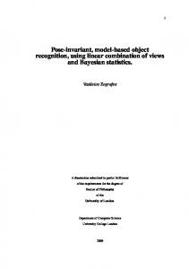
Understanding the properties of feature distributions represents an important step in the path towards achieving efficient image feature self-organization. The challenge posed by this task resides in the intrinsic complexity of high dimensional data spaces and the lack of prior knowledge about the topological characteristics of their manifolds. The image feature matching mechanism inherent to the learning and recall procedures of the Neural Map, described in Section 3.3, depends on a nearest neighbor search in the approximated manifold of the feature domain, where the candidate neurons are ranked according to the measure of distance defined in Section 3.1. This mechanism involves the implicit assumption that the image features naturally form groups that share common statistical characteristics, and in the context of unsupervised learning they follow a natural distribution [42]. In Section 4.4, the present work applies the unsupervised self-organization properties of the Enhanced Tree Growing Neural Gas (ETreeGNG) algorithm to corroborate the existence of these groups in four feature distributions. The related clustering experiments are based on a complete data set FSB of borderline Square image features, defined in Section 2.2, which are derived from the object views of the ETH-80 image set (close-perimg version). These image features provide 5 feature vectors, denominated Gabor jets, that comprise 40 feature descriptors obtained with the Γ discrete Gabor filter family. The feature descriptors of each Gabor jet are extracted from the object views at locations, defined with the Grid key-point detector, as specified in Section 2.3. In line with the findings of Richter [72], resulting from applying the ETreeGNG to the texture information of Square image features, the representative clustering scheme of the feature distribution FSSB is one large cluster containing most of the neurons in the Growing Neural Gas (GNG) network. The cluster composition is distributed extremely uneven across all basic level categories, as described in Table 4.2. The qualitative validation of this clustering scheme using external testing criteria [102] attains low R and J, and medium F M values for the superordinate areas as well as for the basic level categories, and the Γ statistics cannot be calculated. The challenge of clustering image features with the ETreeGNG algorithm is connected to the so-called curse of dimensionality [6, 42]. It argues that potentially redundant and irrelevant feature descriptors of the samples decrease the contrast between nearest and farthest neighbors on the approximated manifold and, thus, the ETreeGNG algorithm is unable to generate meaningful clustering schemes of the feature distribution. In order to overcome the curse of dimensionality, the present work generates two embedded distributions, with lower-dimensional samples that only retain the relevant feature descriptors. One embedded feature distribution FSSPB results from the Principal Component Analysis (PCA) of the feature distribution FSSB , de-

115

CHAPTER 6. DISCUSSION scribed in Section 4.3.1. The other one FSSM is created by applying the Modified Locally Linear B S

Embedding (MLLE) to prototype samples from a quantized distribution FSQB of the feature distribution FSSB , as detailed in Section 4.3.2. On the one hand, the clustering scheme of the embedded distribution FSSPB is also composed of a single cluster. Although the distribution of its neurons among the basic level categories is smoother, the qualitative evaluation of this clustering scheme is equivalent to the one obtained for the feature distribution FSSB . On the other hand, the clustering scheme of the embedded distribution FSSM contains multiple clusters. The biggest one represents 81.62% of the GNG B network, with a widely distributed composition, but favoring the animals basic level categories (i.e., cows, dogs, and horses). The other clusters are smaller, with 0.37% to 13.79% of the remaining neurons, and predominantly labeled with fruits and vegetables (i.e., apples, pears, and tomatoes), or human made small (i.e., cups) basic level categories. The qualitative evaluation of the clustering scheme of the embedded distribution FSSPM has the best experimental results, with medium R and F M , and low J and Γ values registered for all the abstraction levels. S

In general, the clustering schemes resulting from applying the ETreeGNG to the FSSB , FSQB , feature distributions are not meaningful enough to shape hierarchical artificial sysand FSSM B tems built upon their approximations, such as the Neural Map Hierarchy (NMH) defined in Section 3.4. Nonetheless, the PCA and MLLE dimensionality reduction approaches successfully increase the difference between nearest and the farthest neighbors on the manifold, as depicted in Figure 6.1. The relevance of the nearest neighbor search also improves in both cases according to the Significance Criterion [50] (SC) and the Fisher’s discriminant ratio [22] (FDR) values, which are illustrated in Figure 5.4 and Figure 5.5 respectively. Moreover, the representation of some basic level categories over others in the clustering schemes of the quantized distribution S

FSQM and its embedded one FSSPM could be related to the order of the image features established during the quantization process, which is defined in Section 4.2. Finally, the on-line and off-line labeling approaches of the ETreeGNG have equivalent results, which evidence the preservation of the relationships between the samples from the feature distributions and the neurons of the developed GNG network during the self-organization process described in Section 3.2. The present work also cross-compares the novel object categorization performance of the Neural Map Classifier (NMC) based on the feature, quantized, and their embedded distributions in Section 5.7. The experimental results displayed in Table 5.14 indicate a decreasing tendency of the overall correct categorization percentages of the NMC utilizing the embedded distributions in comparison to the ones observed for their originating feature and quantized distributions. However, the detailed results of these experiments, shown in Table B.18, revert this tendency for the natural superordinate areas (i.e., fruits and vegetables, and animals). Nevertheless, the combination of both results suggests that the improvement of the separabil116


NN-FN

NN-FN [P]

1600

20000

1200

15000

800

10000

Frequency

400 0

5000

0.60

0.66

0.72

0.78

0.84

0.90

0.96

0

1.824

1.848

1.872

NN-FN [Q] 800

600

600

400

400

200

200

0.495

0.550

0.605

0.660

0.715

1.920

1.944

1.968

1.992

NN-FN [M]

800

0

1.896

0.770

0.825

0

1.47

1.54

1.61

1.68

1.75

1.82

1.89

1.96

Figure 6.1: Emergence of Natural Clusters. The difference between the nearest and the farthest S

neighbors in the approximated manifold of samples from the FSSB , FSSPB (P), FSQB (Q), and (M) feature distributions. FSSM B ity in the embedded distributions may not compensate for their loss of information during the NMC’s learning and recall phases.

6.6

Artificial Systems: State of the Art

The Neural Map Classifier (NMC), the Neural Map Hierarchy (NMH), and the Semantic Correlation Graph (SCG) provide the learning and recall mechanisms of feature-based object recognition and categorization systems. The cross-comparison experiments, introduced in Section 5.8, measure the performance of these artificial systems to model object recognition and categorization, utilizing object views of the ETH-80 image set and the COIL-100, as detailed in Section 5.1. In all the experiments of the present work, the learning phase of the three artificial systems completes with zero learning error, ensuring that the training object views are correctly recognized and categorized 100% of the time. In the case of the NMC and the NMH, the learning error should not be mistaken with the Global Error (GE) or the Mean Error (ME), which are values related to the Neural Map’s underlying Growing Neural Gas (GNG) network. These error values accumulate the distance between samples of the feature distribution and their nearest neighbor in the GNG network during self-organization, and are exclusively used to set 117


challenging thresholds in the learning phase (i.e., GET and MET) of the artificial systems. The recall phase of the artificial systems based on the Neural Map memory model (i.e., the NMC and the NMH) uses a partitioning scheme FkR ⊆ FR of the test image features FR , with

k ∈ {1, . . . , 3} levels of abstraction. These partitions group the image features according to

the object’s identity, with k = 1, the object’s view-point, with k = 2, and the object’s feature, with k = 3. These criteria define the amount of texture information the artificial systems can utilize to determine the best matching signature for the object in the probe images. The identity partition F1R emulates visual object understanding using a sequence of snapshots from the object, similar to how an infant would scrutinize a new toy to identify its properties; the view-point partition F2R does it with a single snapshot of this sequence; and the feature partition F3R with one object part taken from one snapshot. In comparison to these two artificial systems, the recall phase of the Semantic Correlation Graph (SCG) only utilizes the texture information of the view-point partition F2R of the test image features. The experimental results listed in Table 5.16 cross-compare the incremental-hold-out validation of the three artificial systems using object views of the ETH-80 image set. In general, the NMC/F1R outperforms the other approaches almost all partitions of the complete data set, with the exception of the one using 90% of the view-points during the learning phase and 10% in the recall phase. The SCG attains the highest recognition percentages when excluding the NMC/F1R and NMH/F1R results from the cross-comparison. In these experiments, the artificial systems based on the Neural Map have equivalent results for the superordinate areas. However, the correct recognition percentages registered for basic level categories and object identity abstraction levels slightly favor the NMC over the NMH, unless the experiment uses a complete data set partition with few view-points in the learning phase (e.g., 10% or 30% of the total view points). It is worth noting that, due to the unbalanced nature of ETH-80 object taxonomy (e.g., the superordinate area fruits and vegetables comprises 1230 images from 30 objects, while human made big has 410 images from 10 objects), the used neural growth and bootstrapping limits, defined in Table 5.7, translate to different number of neurons in the resulting Neural Maps of the superordinate areas, as detailed in Table 5.19. Nonetheless, these limits represent the same ratio to the total amount of texture information available during learning. Additionally, the results of the invariant object recognition experiments with the object views of the ETH-80 image set are particularized to the basic level categories and crosscompared to the ones of three hierarchical neural network approaches. The Temporal Correlation Graph [55] (TCG) is composed of three layers, each of which contains a spatial and a temporal sublayer. In the lowest level of this hierarchy, the neurons are represented with prototype image features from a codebook, which are determined using a quantization scheme 118


similar to the one defined in Section 4.2. On the higher levels, each neuron stores its weighted connections, or synapses, to neurons in the level below (e.g., the temporal neurons in the second layer have connections to spatial neurons in the first layer, spatial neurons in the third layer are connected to temporal neurons in the second layer, and so on). The neuron activities are computed on grid positions in the network. In the lowest level, the grid is 9 × 9 positions, which are usually configured to 5 pixels each, in both the spatial and the temporal sublayer.

Similarly, the grid in the second layer is 3 × 3 positions, and the one in the third layer is 1

position. The convergence of the grid sizes determines the spatial proximity in the neural net-

work, while temporal neurons on the grid positions that feed the same position in the next level create the spatial patterns. This approach creates clusters of image features during learning, so-called temporal groups, which are set to the number of categories in the top level of this hierarchy. The Temporal Correlation Network [54] (TCN) is a variation of the TCG, where the configuration of the neurons from the top layer is more versatile, and the synapses can be defined on-line through Hebbian learning. These two approaches use parquet graphs, which are conceptually similar to the medium-sized image features of the present work, but they contain nearly twice the amount of feature descriptors. The Hierarchical Temporal Memory [33] (HTM) is also a converging hierarchy of neurons that learns temporal sequences to generate invariant object representations. However, its neurons learn localized codebooks of image features with a fixed size, instead of having a single global codebook of prototype features like the TCG/TCN. Furthermore, this approach uses image features represented with Gabor functions, which are extracted from the probe images scaled to a size of 200 × 200 pixels.

The overall results for the incremental-hold-out validation of these artificial systems, sum-

marized in Table 5.17, indicate that the NMH/F1R has the highest correct recognition percentages when 10% of the view-points are available in the learning phase and 90% in the recall phase. The NMC/F1R and the TCN present comparable results in most of the other partitions of complete data set, excepting the one with 90% of view-points used during learning and 10% for recall. In this particular case, the TCN has the highest correct recognition percentages, closely followed by the ones obtained employing the SCG. The performance of the artificial systems for invariant object recognition is also evaluated using object views of the COIL-100. In these experiments, the NMH has a flat hierarchy composed of one Neural Map at the universal abstraction level, since the images of the COIL-100 only provide object identities as ground truth, making both Neural Map based artificial systems structurally equivalent. The cross-comparison of the results obtained for this image library using the artificial systems of the present work includes the ones of the TCG, the TCN, and two additional approaches. The Feature-and-correspondence-based Pattern Recognizers [95] (FCPR) combines a feed-forward neural network with a form of graph dynamics to assemble 119


model graph candidates from a set of Parquet graphs. Then, it matches these candidates to the probe image, using a simplified version of of Elastic Graph Matching (EGM) [50], and selects the one located with the highest similarity. The Composed Complex-cue Histograms [56] (CCH) calculates one histogram of different combinations of image features for every probe image. These features are based on Gaussian derivatives or differential invariants, applied to either intensity information, color-opponent channels, or both. The generated histograms are classified through a nearest neighbor search, with the χ2 -measure, or a kernel based support vector machine (SVM). Table 5.18 details the incremental-hold-out validation results of these experiments for the artificial systems of the present work, the TCG, the TCN, and the CCH together with the fivefold cross-validation results of the image library using the FCPR. In this case, the correct object recognition percentages of the NMC/NMH/F1R are the highest ones of all partitions of the complete data set. If only the other abstraction levels of the NMC/NMH recall phase are taken into consideration (i.e., F2R and F3R ), then the SCG outperforms or matches the results of all the other artificial systems in most partitions, excepting the one that uses 90% view-points for the learning phase and 10% for the recall phase. The performance for novel object categorization of the artificial systems is evaluated with the leave-one-out cross-validation of object views from the ETH-80 image set. The crosscomparison experiments based on this evaluation paradigm include the results of the NMC, the NMH, the SCG, the TCG, the FCPR, and two supplementary approaches. The Kernel Combination [81] (KC) defines a kernel with the product of labeled graphs, which describe the morphological skeleton of the objects, and local histograms of gradients, which capture the the appearance of the objects, and uses a SVM classifier to categorize an object. The Multi-cue Decision Tree [53] (MCDT) combines categorization methods using color, texture, and shape information of the object views into a decision tree based on their performance for each category. The color method collects global Red Green Blue (RGB) histograms and compares them with the χ2 -measure; the texture method employs the Dx Dy and the Mag-Lap, which are variations of histograms containing local gray value derivatives at multiple scales; and the shape method applies the Principal Component Analysis (PCA) to the object’s segmentation mask to capture the global shape, and utilizes images with the object’s contour to represent the local shape. The overall results of the leave-one-out cross-validation, listed in Table 5.21, favor the NMC/NMH/F1R for the superordinate areas, and the NMC/F1R for the basic level categories. However, if the results obtained with the F1R partition are neglected, then the SCG achieves the highest categorization percentages for the superordinate areas, and the TCG for the basic level categories. In this case, the results of the NMC/F2R and NMC/F3R can be improved (i.e., 95.9 for NMC/F2R and 78.18 for NMC/F3R in the superordinate areas, as well as 76.57 for NMC/F2R and 120

CHAPTER 6. DISCUSSION 52.73 for NMC/F3R in the basic level categories) using alternative local feature representations, as demonstrated in Table 5.11. A related point to consider is that, compared to the KC and the MCDT, which use multiple-cues, the other artificial systems only use texture information to categorize the object views. The results of these novel object categorization experiments are further detailed for every object signature of both abstraction levels in Table 5.21. Taking a closer look, contrary to the overall results, the TCG, KC, and MCDT outperform the SCG for human made small; and they show similar results for human made big. Moreover, the MCDT has the best results for cows, followed by the TCG, which also presents the highest categorization percentages for horses. The rest of the object signatures from the superordinate areas and the basic level categories preserve the tendencies observed in the overall results.

6.6.1

General Remarks

The variations of the SCG, which evaluate alternative values for the input weight W defined in Section 3.5, produce comparable results in all the experiments of the present work. However, relatively balanced weight distributions (e.g., W0.4 , W0.6 , and W0.8 ) slightly outperform the more extreme ones (i.e., W0.0 and W1.0 ) in the majority of the cases. Regarding the partitioning scheme FkR of the test image features used in the recall phase of the Neural Map based artificial systems, all the experimental results consistently indicate that the more abstract groupings of the texture information facilitate the modeling of visual object understanding in comparison to the more concrete ones. Moreover, the scarcity of texture information in the F3R partition of the test image features leads to the lowest recognition and categorization percentages in all the experiments. Indeed, capturing the representation of an object with five Gabor jets is a very hard task to accomplish, considering the high similarity that one Gabor jet has on most locations of the probe image [36]. Nonetheless, the analysis of the performance differences for novel feature retrieval between artificial systems provides an insight on their accuracy to match single image features. The mechanism introduced to minimize propagation of early made errors in the coarse to fine voting process of the NMH proves to be successful. This outcome is also replicated to the winner-take-all voting scheme of the NMC. The improvement of this mechanism is mostly evident by contrasting the correct object recognition and categorization percentages of the human made small superordinate area and the cups basic level category.

121

Chapter 7 Conclusion and Further Research The present work introduces a memory framework for object recognition and categorization systems based on dynamically assembled object models [94]. The properties of the proposed computational theory are grounded in the unsupervised structural organization of these object models’ components according to their visual resemblance and co-occurrence, as well as in the use of this structure for matching the novel components. Both have been identified as important for achieving efficient object recognition and categorization and for providing insight on the knowledge-driven aspect of perception [19]. These foundations are materialized in three different approaches to the self-organization of visual object knowledge: the Neural Map, the Neural Map Hierarchy (NMH), and the Semantic Correlation Graph (SCG). Donatti and W¨ urtz [20] combine a Growing Neural Gas (GNG) Network [29, 30] and a classifier inspired by the coding and decoding of information in the brain [85] within a socalled Neural Map. The proficiency of this memory model to self-organize texture information is put to the test by integrating its feature matching responses with a winner-take-all voting scheme. In these experiments, the performance for object recognition and categorization of the resulting Neural Map Classifier (NMC) is validated using image features that derive texture information from object views with different granularity. The present work extends them to borderline Square image features employing different representations to encode gray- and colorvalued texture information from object views. It also evaluates alterations on self-organization caused by neural network bootstrapping [10]. The overall results indicate that medium-sized image features with the highest amount of feature descriptors maximize the informativeness and distinctiveness of texture information derived from object views. Furthermore, bootstrapping neural network topologies enhances the artificial system’s performance at the cost of slightly longer learning times. The optimization paradigm introduced in Donatti et al. [21] identifies the parameter values of the Neural Map that are best suited for object recognition and categorization. This paradigm 122

CHAPTER 7. CONCLUSION AND FURTHER RESEARCH

is based on Evolutionary Algorithms [2, 40] (EAs) and explores six different optimization approaches given by the combination of three fitness functions and two starting conditions. The parameter values obtained from the fittest individuals of these approaches are cross-compared and cross-validated with empirical ones using a more elaborate version of the experimental protocol defined in Donatti and W¨ urtz [20]. The parameter values determined with the Sample Distance (SD) fitness function generate Neural Maps that attain the highest object recognition and categorization percentages. The present work also implements bootstrapping and neural growth limits during learning to demonstrate the Neural Map capabilities for data compression. The search for the fittest individuals encounters two limitations that could be resolved in future research. The first one relates to the computational complexity of training and evaluating large GNG networks using high dimensional image features. This is particularly observed when employing a combination of Global Error (GE) and SD fitness functions with empirical (Emp) starting conditions, which favor individuals that lead to large GNG networks. The evolution of a generation using these processing-intensive approaches can become computationally intractable. The second limitation is the poor ability of the fitness functions to favor the saliency of individuals that may generate better approximations of the feature distribution topology. Donatti et al. [21] introduces the Growth Restriction (GR) to overcome the first limitation, but empirically it is too restrictive, and Neural Maps using this approach are experimentally the least performing ones. As an alternative, the number of generations needed to find an optimal individual can be reduced with a method based on the Covariance Matrix Adaptation (CMA) [39, 82]. However, CMA only optimizes continuous values and, therefore, has to be adapted for discontinuous ones in order to be used with the approach presented in Donatti et al. [21]. Employing CMA might also allow for the use of the CMA for Multiobjective Optimization [45] to restrict the growth rates of the GNG networks. Concerning the second limitation, the optimization process may be improved using additional fitness functions to assess the learning capabilities of a GNG network (e.g., assigning lower fitness values for errors generated in later generations and disregarding errors in earlier ones, or incorporating a rate of change observed in the global error curve of the GNG algorithm). The NMH is motivated by the efficiency to store and retrieve semantic information of taxonomic hierarchies and by the idea that the cognitive system exploits the tendency of features to occur in clusters across instances in the world. This memory model comprises different abstraction layers with self-organized representations of categories. The representations approximate the topological properties of clusters containing semantically equivalent samples of the feature distribution. The information stored in the more general representations determines the feature weights of more specific levels of categorization. The hierarchy of this memory model is defined according to the taxonomy of the ETH-80 image set [53]. The present work also stud123

CHAPTER 7. CONCLUSION AND FURTHER RESEARCH

ies alternatives employing emergent structures from the unsupervised clustering of the feature distribution using the Enhanced Tree Growing Neural Gas [72] (ETreeGNG). These experiments overcome the curse of dimensionality [6] through data quantization and dimensionality reduction techniques, such as Principal Component Analysis [69] (PCA) and Modified Locally Linear Embedding [104] (MLLE), which are tailored [13, 87] to the properties of the feature distribution. Although external validation criteria [102] and data separability [22, 50] improve in these embedded distributions, the resulting clustering schemes are not meaningful enough to shape the hierarchy of the NMH. It is worth noting that while using absolute values of feature distances may not be reliable due to the curse of dimensionality, which relates to the challenge of clustering the feature distribution, it is still viable to use rankings of these values for object recognition and categorization [42]. Further research in this line of work could apply the MLLE algorithm to non-quantized versions of the feature distribution, provided there are suitable hardware conditions available, or to quantize it with more robust approaches. Additionally, it could also modify the MLLE algorithm utilizing the normalized scalar product instead of the Euclidean distance to define the neighborhoods. Finally, it could also replicate the clustering experiments of the present work with image feature representations that are not based on responses from discrete Gabor filter families, and/or using alternative image libraries having more object categories. The SCG self-organizes image features depending on their co-occurrence in object views. It employs a configurable weight distribution between occurrences and co-occurrences of image features. The results obtained with different values for this weight distribution are comparable. The performance of feature-based object recognition and categorization systems equipped with the memory framework introduced in the present work are cross-compared to the ones of state-of-the-art approaches found in literature [33, 53–56, 81, 94, 95] utilizing the ETH-80 image set and the COIL-100 [66]. In general, the results for the ETH-80 image set show a gradual decrease of accuracy from the more abstract to the more concrete levels of the taxonomy, reinforcing the concept that the categories from higher abstraction levels are more accurately differentiable, since the characteristics shared by their intra-category individuals are significantly dissimilar in comparison to the ones observed inter-category. In both cases, the artificial systems that employ sequences of object views, either during learning or recall phases, attain the highest object recognition and categorization, in agreement with the intuitive interpretation of visual object understanding in biological systems. An important remark is that the categorization experiments of the present work are obtained through a best case analysis, because novel object views are processed under the same viewing conditions as during training, with near-perfect object segmentation and known scales. Further research should focus on recognition and categorization in more realistic scenes [26, 41]. 124

Bibliography [1] E. Anderson, Z. Bai, C. Bischof, S. Blackford, J. Demmel, J. Dongarra, J. Du Croz, A. Greenbaum, S. Hammarling, A. McKenney, and D. Sorensen. LAPACK Users’ Guide. Society for Industrial and Applied Mathematics, Philadelphia, PA, third edition, 1999. ISBN 0-89871-447-8 (paperback). [2] Thomas Bäck. Evolutionary Algorithms in Theory and Practice. PhD thesis, University of Dortmund, Department of Computer Science, February 1994. [3] Marek Barwi´ nski. A Neurocomputational Model of Memory Acquisition for Novel Faces. PhD thesis, International Graduate School of Neuroscience, Ruhr-Universität Bochum, 2008. [4] Mark F. Bear, Barry W. Connors, and Michael A. Paradiso. Neuroscience: Exploring the Brain. Lippincott Williams & Wilkins, third edition edition, 2006. ISBN 0781760038. [5] Hans-Georg Beyer and Hans-Paul Schwefel. Evolution strategies - A comprehensive introduction. Natural Computing, 1(1):3–52, 2002. doi: 10.1023/A:1015059928466. URL http://dx.doi.org/10.1023/A:1015059928466. [6] Kevin S. Beyer, Jonathan Goldstein, Raghu Ramakrishnan, and Uri Shaft. When is “nearest neighbor” meaningful? In Catriel Beeri and Peter Buneman, editors, Database Theory - ICDT ’99, 7th International Conference, Jerusalem, Israel, January 10-12, 1999, Proceedings., volume 1540 of Lecture Notes in Computer Science, pages 217–235. Springer, 1999. ISBN 3-540-65452-6. doi: 10.1007/3-540-49257-7 15. URL http://dx. doi.org/10.1007/3-540-49257-7_15. [7] Oliver Beyer and Philipp Cimiano. Online labelling strategies for growing neural gas. In Hujun Yin, Wenjia Wang, and Victor J. Rayward-Smith, editors, Intelligent Data Engineering and Automated Learning - IDEAL 2011 - 12th International Conference, Norwich, UK, September 7-9, 2011. Proceedings, volume 6936 of Lecture Notes in Computer Science, pages 76–83. Springer, 2011. ISBN 978-3-642-23877-2. doi: 10.1007/ 978-3-642-23878-9 10. URL http://dx.doi.org/10.1007/978-3-642-23878-9_10. 125

BIBLIOGRAPHY

[8] Oliver Beyer and Philipp Cimiano. Online semi-supervised growing neural gas. Int. J. Neural Syst., 22(5), 2012. doi: 10.1142/S0129065712500232. URL http://dx.doi.org/ 10.1142/S0129065712500232. [9] Irving Biederman. Recognition-by-components: A theory of human image understanding. Psychological Review, 94:115–147, 1987. [10] Bram Bolder. Sensomotorische Koordination eines Roboterkopfes. Shaker, Aachen, 2006. [11] Joachim Buhmann, Jörg Lange, and Christoph von der Malsburg. Distortion invariant object recognition by matching hierarchically labeled graphs. In IJCNN, pages 155–159. IEEE, 1989. [12] Heinrich H. B¨ ulthoff and Shimon Edelman. Psychophysical support for a 2-D view interpolation theory of object recognition. Proceedings of the National Academy of Science of the United States of America, 89:60–64, 1992. [13] Raymond B. Cattell. The scree test for the number of factors. Multivariate Behavioral Research, 1(2):245–276, 1966. doi: 10.1207/s15327906mbr0102\ 10. [14] Allan M. Collins and M. Ross Quillian. Retrieval time from semantic memory. Journal of verbal learning and verbal behavior, 8(2):240–247, 1969. [15] Leonardo Dagum and Ramesh Menon. Openmp: An industry-standard api for sharedmemory programming. IEEE Comput. Sci. Eng., 5(1):46–55, January 1998. ISSN 10709924. doi: 10.1109/99.660313. URL http://dx.doi.org/10.1109/99.660313. [16] John G. Daugman. Uncertainty relation for resolution in space, spatial frequency, and orientation optimized by two-dimensional visual cortical filters. Journal of the Optical Society of America A, 2(7):1160–1169, July 1985. [17] Dick de Ridder and Robert P.W. Duin. Locally linear embedding for classification. Pattern Recognition Group, Dept. of Imaging Science & Technology, Delft University of Technology, Delft, The Netherlands, Tech. Rep. PH-2002-01, pages 1–12, 2002. [18] Kevin Doherty, Rod Adams, and Neil Davey. Treegng - hierarchical topological clustering. In ESANN, pages 19–24, 2005. [19] Guillermo S. Donatti and Rolf P. W¨ urtz. Memory organization for invariant object recognition and categorization. In Brazilian Symposium on Computer Graphics and Image Processing, 20. (SIBGRAPI), pages 11–12. Sociedade Brasileira de Computa¸caõ, October 2007. 126

BIBLIOGRAPHY

[20] Guillermo S. Donatti and Rolf P. W¨ urtz. Using growing neural gas networks to represent visual object knowledge. In ICTAI, pages 54–58. IEEE Computer Society, 2009. ISBN 978-0-7695-3920-1. [21] Guillermo S. Donatti, Oliver Lomp, and Rolf P. W¨ urtz. Evolutionary optimization of growing neural gas parameters for object categorization and recognition. In IJCNN, pages 1862–1869. IEEE, 2010. ISBN 978-1-4244-6916-1. [22] Richard O. Duda, Peter E. Hart, and David G. Stork. Pattern Classification (2nd Edition). Wiley-Interscience, 2000. ISBN 0471056693. [23] Martin C. M. Elliffe, Edmund T. Rolls, and Simon M. Stringer. Invariant recognition of feature combinations in the visual system. Biological Cybernetics, 86(1):59–71, 2002. [24] Boris Epshtein and Shimon Ullman. Semantic hierarchies for recognizing objects and parts. In CVPR. IEEE Computer Society, 2007. [25] Julien Fauqueur, Nick G. Kingsbury, and Ryan Anderson. Multiscale keypoint detection using the dual-tree complex wavelet transform. In Proceedings of the International Conference on Image Processing, ICIP 2006, October 8-11, Atlanta, Georgia, USA, pages 1625–1628. IEEE, 2006. doi: 10.1109/ICIP.2006.312656. [26] Li Fei-Fei, R. Fergus, and P. Perona. Learning generative visual models from few training examples: An incremental bayesian approach tested on 101 object categories. In Computer Vision and Pattern Recognition Workshop, 2004. CVPRW ’04. Conference on, pages 178–178, June 2004. doi: 10.1109/CVPR.2004.109. [27] E. B. Fowlkes and C. L. Mallows. A method for comparing two hierarchical clusterings. Journal of the American Statistical Association, 78(383):553–569, 1983. ISSN 01621459. URL http://www.jstor.org/stable/2288117. [28] Bernd Fritzke. Growing cell structures–a self-organizing network for unsupervised and supervised learning. Neural Networks, 7(9):1441–1460, 1994. doi: 10.1016/0893-6080(94) 90091-4. [29] Bernd Fritzke. A growing neural gas network learns topologies. In Gerald Tesauro, David S. Touretzky, and Todd K. Leen, editors, Advances in Neural Information Processing Systems 7, [NIPS Conference, Denver, Colorado, USA, 1994], pages 625–632. MIT Press, 1994.

127

BIBLIOGRAPHY

[30] Bernd Fritzke. A self-organizing network that can follow non-stationary distributions. In Wulfram Gerstner, Alain Germond, Martin Hasler, and Jean-Daniel Nicoud, editors, Artificial Neural Networks - ICANN ’97, 7th International Conference, Lausanne, Switzerland, October 8-10, 1997, Proceedings, volume 1327 of Lecture Notes in Computer Science, pages 613–618. Springer, 1997. ISBN 3-540-63631-5. doi: 10.1007/BFb0020222. [31] Kunihiko Fukushima, Sei Miyake, and Takayuki Ito. Neocognitron: A neural network model for a mechanism of visual pattern recognition. IEEE Transactions on Systems, Man, and Cybernetics, 13(5):826–834, 1983. [32] Dennis Gabor. Theory of communications. Journal of the Institution of Electrical Engineers, 98:429457, 1946. [33] Dileep George and Jeff Hawkins. Towards a mathematical theory of cortical micro-circuits. PLoS Computational Biology, 5(10), 2009. doi: 10.1371/journal.pcbi.1000532. URL http: //dx.doi.org/10.1371/journal.pcbi.1000532. [34] Daniel González-Jiménez, Manuele Bicego, Johan W. H. Tangelder, Ben A. M. Schouten, Onkar Ambekar, José Luis Alba-Castro, Enrico Grosso, and Massimo Tistarelli. Distance measures for gabor jets-based face authentication: A comparative evaluation. In SeongWhan Lee and Stan Z. Li, editors, Advances in Biometrics, International Conference, ICB 2007, Seoul, Korea, August 27-29, 2007, Proceedings, volume 4642 of Lecture Notes in Computer Science, pages 474–483. Springer, 2007. ISBN 978-3-540-74548-8. doi: 10.1007/ 978-3-540-74549-5 50. URL http://dx.doi.org/10.1007/978-3-540-74549-5_50. [35] Kristen Grauman and Bastian Leibe. Visual object recognition. Synthesis Lectures on Artificial Intelligence and Machine Learning, 5(2):1–181, 2011.

doi:

10.2200/

S00332ED1V01Y201103AIM011. [36] Manuel G¨ unther. Statistical Gabor Graph Based Techniques for the Detection, Recognition, Classification, and Visualization of Human Faces. PhD thesis, Computer Science, Univ. of Ilmenau, Germany, 2012. [37] Manuel G¨ unther and Rolf P. W¨ urtz. Face detection and recognition using maximum likelihood classifiers on gabor graphs. IJPRAI, 23(3):433–461, 2009. [38] Manuel G¨ unther, Stefan Böhringer, Dagmar Wieczorek, and Rolf P. W¨ urtz. Reconstruction of images from gabor graphs with applications in facial image processing. International Journal of Wavelets, Multiresolution and Information Processing, 13(3), 2015.

128

BIBLIOGRAPHY

[39] Nikolaus Hansen and Andreas Ostermeier. Completely derandomized self-adaptation in evolution strategies. Evolutionary Computation, 9(2):159–195, 2001. doi: 10.1162/ 106365601750190398. URL http://dx.doi.org/10.1162/106365601750190398. [40] John H. Holland. Adaptation in Natural and Artificial Systems: An Introductory Analysis with Applications to Biology, Control and Artificial Intelligence. MIT Press, Cambridge, MA, USA, 1992. ISBN 0262082136. [41] Sebastian Houben, Johannes Stallkamp, Jan Salmen, Marc Schlipsing, and Christian Igel. Detection of traffic signs in real-world images: The german traffic sign detection benchmark. In The 2013 International Joint Conference on Neural Networks, IJCNN 2013, Dallas, TX, USA, August 4-9, 2013, pages 1–8. IEEE, 2013. ISBN 978-1-46736128-6. doi: 10.1109/IJCNN.2013.6706807. URL http://dx.doi.org/10.1109/IJCNN. 2013.6706807. [42] Michael E. Houle, Hans-Peter Kriegel, Peer Kröger, Erich Schubert, and Arthur Zimek. Can shared-neighbor distances defeat the curse of dimensionality?

In Michael Gertz

and Bertram Ludäscher, editors, Scientific and Statistical Database Management, 22nd International Conference, SSDBM 2010, Heidelberg, Germany, June 30 - July 2, 2010. Proceedings, volume 6187 of Lecture Notes in Computer Science, pages 482–500. Springer, 2010. ISBN 978-3-642-13817-1. doi: 10.1007/978-3-642-13818-8 34. URL http://dx. doi.org/10.1007/978-3-642-13818-8_34. [43] David H. Hubel and Torsten N. Wiesel. Receptive fields, binocular interaction and functional architecture in the cat’s visual cortex. Journal of Physiology, 160:106–154, 1962. [44] C. Igel, V. Heidrich-Meisner, and T. Glasmachers. Shark. The Journal of Machine Learning Research, 9:993–996, 2008. [45] Christian Igel, Nikolaus Hansen, and Stefan Roth. Covariance matrix adaptation for multi-objective optimization. Evolutionary Computation, 15(1):1–28, 2007. doi: 10.1162/ evco.2007.15.1.1. URL http://dx.doi.org/10.1162/evco.2007.15.1.1. [46] Judson P. Jones and Larry A. Palmer. An evaluation of the two-dimensional gabor filter model of simple receptive fields in cat striate cortex. Journal of Neurophysiology, 58(6): 1233–1258, 1987. [47] Joni-Kristian Kamarainen, Ville Kyrki, and Heikki Kälviäinen. Invariance properties of gabor filter-based features-overview and applications. IEEE Transactions on Image Processing, 15(5):1088–1099, 2006. 129

BIBLIOGRAPHY

[48] Teuvo Kohonen. Self-organized formation of topologically correct feature maps. Biological Cybernetics, 43:59–69, 1982. [49] Norbert Kr¨ uger, Michael Pötzsch, and Christoph von der Malsburg. Determination of face position and pose with a learned representation based on labelled graphs. Image and Vision Computing, 15(8):665–673, 1997. [50] Martin Lades, Jan C. Vorbr¨ uggen, Joachim M. Buhmann, Jörg Lange, Christoph von der Malsburg, Rolf P. W¨ urtz, and Wolfgang Konen. Distortion invariant object recognition in the dynamic link architecture. IEEE Trans. Computers, 42(3):300–311, 1993. [51] D. T. Lee and Bruce J. Schachter. Two algorithms for constructing a delaunay triangulation. International Journal of Parallel Programming, 9(3):219–242, 1980. doi: 10.1007/BF00977785. [52] Tai Sing Lee. Image representation using 2d gabor wavelets. IEEE Trans. Pattern Anal. Mach. Intell., 18(10):959–971, 1996. [53] Bastian Leibe and Bernt Schiele. Analyzing appearance and contour based methods for object categorization. In CVPR (2), pages 409–415. IEEE Computer Society, 2003. ISBN 0-7695-1900-8. [54] Markus Leßmann and Rolf P. W¨ urtz. Online learning of invariant object recognition in a hierarchical neural network. In Stefan Wermter, Cornelius Weber, Wlodzislaw Duch, Timo Honkela, Petia D. Koprinkova-Hristova, Sven Magg, G¨ unther Palm, and Alessandro E. P. Villa, editors, Artificial Neural Networks and Machine Learning ICANN 2014 - 24th International Conference on Artificial Neural Networks, Hamburg, Germany, September 15-19, 2014. Proceedings, volume 8681 of Lecture Notes in Computer Science, pages 427–434. Springer, 2014. ISBN 978-3-319-11178-0. doi: 10.1007/ 978-3-319-11179-7 54. URL http://dx.doi.org/10.1007/978-3-319-11179-7_54. [55] Markus Leßmann and Rolf P. W¨ urtz. Learning invariant object recognition from temporal correlation in a hierarchical network. Neural Networks, 54:70–84, 2014. doi: 10.1016/j. neunet.2014.02.011. URL http://dx.doi.org/10.1016/j.neunet.2014.02.011. [56] Oskar Linde and Tony Lindeberg. Composed complex-cue histograms: An investigation of the information content in receptive field based image descriptors for object recognition. Computer Vision and Image Understanding, 116(4):538–560, 2012. doi: 10.1016/j.cviu. 2011.12.003. URL http://dx.doi.org/10.1016/j.cviu.2011.12.003.

130

BIBLIOGRAPHY

[57] Ralph Linsker. Self-organization in a perceptual network. IEEE Computer, 21(3):105– 117, 1988. [58] Oliver Lomp. Finding optimal parameters for neural networks using evolutionary algorithms. B.Sc. Thesis, ET-IT Dept., Univ. of Bochum, Germany, October 2008. [59] David G. Lowe. Object recognition from local scale-invariant features. In ICCV, pages 1150–1157, 1999. doi: 10.1109/ICCV.1999.790410. [60] David G. Lowe. Distinctive image features from scale-invariant keypoints. International Journal of Computer Vision, 60(2):91–110, 2004. doi: 10.1023/B:VISI.0000029664.99615. 94. [61] Bruce MacLennan. Gabor representations of spatiotemporal visual images. Technical report, Knoxville, TN, USA, 1991. [62] Thomas Martinetz. Competitive hebbian learning rule forms perfectly topology preserving maps. In S. Gielen and B. Kappen, editors, Proceedings of the International Conference on Artificial Neural Networks (ICANN-93), Amsterdam, pages 427–434, Heidelberg, 1993. Springer. [63] Thomas Martinetz and Klaus Schulten. A “Neural-Gas” Network Learns Topologies. Artificial Neural Networks, I:397–402, 1991. [64] Thomas Martinetz and Klaus Schulten. Topology representing networks. Neural Networks, 7(3):507–522, 1994. doi: 10.1016/0893-6080(94)90109-0. [65] Hiroshi Murase and Shree K. Nayar. Visual learning and recognition of 3-d objects from appearance. International Journal of Computer Vision, 14(1):5–24, 1995. [66] Sameer A. Nene, Shree K. Nayar, and Hiroshi Murase. Columbia Object Image Library (COIL-100). Technical report, February 1996. [67] Bruno A. Olshausen and David J. Field. Emergence of simple-cell receptive field properties by learning a sparse code for natural images. Nature, 381(6583):607–609, 1996. [68] Thomas J. Palmeri and Isabel Gauthier. Visual object understanding. Nature Reviews Neuroscience, 5(4):291–303, 2004. [69] Karl Pearson. Liii. on lines and planes of closest fit to systems of points in space. Philosophical Magazine Series 6, 2(11):559–572, 1901. doi: 10.1080/14786440109462720.

131

BIBLIOGRAPHY

[70] P. Jonathon Phillips, Patrick J. Flynn, W. Todd Scruggs, Kevin W. Bowyer, Jin Chang, Kevin Hoffman, Joe Marques, Jaesik Min, and William J. Worek. Overview of the face recognition grand challenge. In CVPR (1), pages 947–954. IEEE Computer Society, 2005. ISBN 0-7695-2372-2. [71] William M. Rand. Objective criteria for the evaluation of clustering methods. Journal of the American Statistical Association, 66(336):846–850, 1971. ISSN 01621459. URL http://www.jstor.org/stable/2284239. [72] Mathis Richter. Using enhanced tree growing neural gas networks to represent knowledge derived from artificial and real-world data. B.Sc. Thesis, ET-IT Dept., Univ. of Bochum, Germany, November 2009. [73] Maximilian Riesenhuber and Tomaso Poggio. Hierarchical models of object recognition in cortex. Nature Neuroscience, 2(11):1019–1025, 1999. [74] Maximilian Riesenhuber and Tomaso Poggio. Cbf: A new framework for object categorization in cortex. In Seong-Whan Lee, Heinrich H. B¨ ulthoff, and Tomaso Poggio, editors, Biologically Motivated Computer Vision, volume 1811 of Lecture Notes in Computer Science, pages 1–9. Springer, 2000. ISBN 3-540-67560-4. [75] Timothy T. Rogers and James L. Mcclelland. Semantic Cognition: A Parallel Distributed Processing Approach. MIT Press, March 2006. ISBN 0262681579. [76] Eleanor Rosch, Carolyn B. Mervis, Wayne D. Gray, David M. Johson, and Penny BoyesBream. Basic objects in natural categories. pages 382–439, 1976. [77] Sam T. Roweis and Lawrence K. Saul. Nonlinear dimensionality reduction by locally linear embedding. Science, 290:2323–2326, 2000. [78] David E. Rumelhart and Peter M. Todd. Learning and connectionist representations. In David E. Meyer and Sylvan Kornblum, editors, Attention and Performance XIV: Synergies in Experimental Psychology, Artificial Intelligence, and Cognitive Neuroscience, pages 3–30. MIT Press, 1993. [79] Bernt Schiele and James L. Crowley. Recognition without correspondence using multidimensional receptive field histograms. International Journal of Computer Vision, 36(1): 31–50, 2000. [80] Thomas Serre, Lior Wolf, Stanley M. Bileschi, Maximilian Riesenhuber, and Tomaso Poggio. Robust object recognition with cortex-like mechanisms. IEEE Trans. Pattern Anal. Mach. Intell., 29(3):411–426, 2007. 132

BIBLIOGRAPHY

[81] Frederic Suard, Alain Rakotomamonjy, and Abdelaziz Bensrhair. Object categorization using kernels combining graphs and histograms of gradients. In Aurélio C. Campilho and Mohamed S. Kamel, editors, Image Analysis and Recognition, Third International Conference, ICIAR 2006, Póvoa de Varzim, Portugal, September 18-20, 2006, Proceedings, Part II, volume 4142 of Lecture Notes in Computer Science, pages 23–34. Springer, 2006. ISBN 3-540-44894-2. doi: 10.1007/11867661 3. URL http://dx.doi.org/10. 1007/11867661_3. [82] Thorsten Suttorp, Nikolaus Hansen, and Christian Igel. Efficient covariance matrix update for variable metric evolution strategies. Machine Learning, 75(2):167–197, 2009. doi: 10.1007/s10994-009-5102-1. URL http://dx.doi.org/10.1007/s10994-009-5102-1. [83] Keiji Tanaka, Hide A. Saito, Yoshiro Fukada, and Madoka Moriya. Coding visual images of objects in the inferotemporal cortex of the macaque monkey. Journal of Neurophysiology, 66:170–189, 1991. [84] Michael J. Tarr and Heinrich H. B¨ ulthoff. Is human object recognition better described by geon-structural-descriptions or by multiple views? Journal of Experimental Psychology: Human Perception and Performance, 21(6):1494–1505, 1995. [85] Thomas Trappenberg. Fundamentals of Computational Neuroscience. Oxford University Press, June 2002. ISBN 0198515839. [86] Shimon Ullman. High-Level Vision: Object Recognition and Visual Cognition. MIT Press, first edition edition, 1996. ´ [87] Juliana Valencia-Aguirre, Andrés Marino Alvarez-Meza, Genaro Daza-Santacoloma, and Germán Castellanos-Dom´ınguez. Automatic choice of the number of nearest neighbors in locally linear embedding. In Eduardo Bayro-Corrochano and Jan-Olof Eklundh, editors, Progress in Pattern Recognition, Image Analysis, Computer Vision, and Applications, 14th Iberoamerican Conference on Pattern Recognition, CIARP 2009, Guadalajara, Jalisco, Mexico, November 15-18, 2009. Proceedings, volume 5856 of Lecture Notes in Computer Science, pages 77–84. Springer, 2009. ISBN 978-3-642-10267-7. doi: 10.1007/ 978-3-642-10268-4 9. URL http://dx.doi.org/10.1007/978-3-642-10268-4_9. [88] Christoph von der Malsburg. Self-Organization of Orientation Sensitive Cells in the Striate Cortex. Kybernetik, 14:85–100, 1973. [89] Christoph von der Malsburg. Pattern recognition by labeled graph matching. Neural Networks, 1(2):141–148, 1988. 133

BIBLIOGRAPHY

[90] Georges Voronoi. Nouvelles applications des paramètres continus a` la théorie des formes quadratiques. deuxième mémoire. recherches sur les parallélloèdres primitifs. Journal f¨ ur die reine und angewandte Mathematik, 134:198–287, 1908. [91] Guy Wallis and Heinrich H. B¨ ulthoff. Learning to recognize objects. Trends in Cognitive Sciences, 3(1):22–31, 1999. [92] Jamie Ward. The Student’s Guide to Cognitive Neuroscience. Psychology Press, first edition edition, 2006. [93] Heiko Wersing and Edgar Körner. Learning optimized features for hierarchical models of invariant object recognition. Neural Computation, 15(7):1559–1588, 2003. [94] G¨ unter Westphal. Feature-Driven Emergence of Model Graphs for Object Recognition and Categorization. PhD thesis, University of L¨ ubeck, Germany, 2006. [95] G¨ unter Westphal and Rolf P. W¨ urtz. Combining feature- and correspondence-based methods for visual object recognition. Neural Computation, 21(7):1952–1989, 2009. [96] Jan Wieghardt, Rolf P. W¨ urtz, and Christoph von der Malsburg. Learning the topology of object views. In Anders Heyden, Gunnar Sparr, Mads Nielsen, and Peter Johansen, editors, ECCV (4), volume 2353 of Lecture Notes in Computer Science, pages 747–760. Springer, 2002. ISBN 3-540-43748-7. [97] Laurenz Wiskott, Jean-Marc Fellous, Norbert Kr¨ uger, and Christoph von der Malsburg. Face recognition by elastic bunch graph matching. IEEE Trans. Pattern Anal. Mach. Intell., 19(7):775–779, 1997. [98] Andrew P. Witkin. Scale-space filtering. In Alan Bundy, editor, Proceedings of the 8th International Joint Conference on Artificial Intelligence. Karlsruhe, FRG, August 1983, pages 1019–1022. William Kaufmann, 1983. [99] Ingo J. Wundrich, Christoph von der Malsburg, and Rolf P. W¨ urtz. Image representation by complex cell responses. Neural Computation, 16(12):2563–2575, 2004. [100] Rolf P. W¨ urtz. Multilayer Dynamic Link Networks for Establishing Image Point Correspondences and Visual Object Recognition. PhD thesis, Fakultät f¨ ur Physik und Astronomie, Ruhr-Universität Bochum, 1994. [101] Rolf P. W¨ urtz. Object recognition robust under translations, deformations, and changes in background. IEEE Trans. Pattern Anal. Mach. Intell., 19(7):769–775, 1997.

134

BIBLIOGRAPHY

[102] Rui Xu and Don Wunsch. Clustering. Wiley-IEEE Press, 2009. ISBN 9780470276808. [103] Kristof Zalecki. Auffinden interessanter bildbereiche mit hilfe der intrinsischen dimensionalität. B.Sc. Thesis, ET-IT Dept., Univ. of Bochum, Germany, May 2011. [104] Zhenyue Zhang and Jing Wang. ing multiple weights.

MLLE: modified locally linear embedding us-

In Bernhard Schölkopf, John C. Platt, and Thomas Hoff-

man, editors, Advances in Neural Information Processing Systems 19, Proceedings of the Twentieth Annual Conference on Neural Information Processing Systems, Vancouver, British Columbia, Canada, December 4-7, 2006, pages 1593–1600. MIT Press, 2006.

ISBN 0-262-19568-2.

URL http://papers.nips.cc/paper/

3132-mlle-modified-locally-linear-embedding-using-multiple-weights.

135

Appendices

136

Appendix A Implementation Details A.1

Hardware Specifications

The experimental results of the present work are calculated over Dell PowerEdge 2900, R710, and R910 computing servers, which are equipped with x64 microprocessors designed and manufactured by Intel Corporation. The first one has two Dual-Core Xeon 5100 processors, with up to 3.0 gigahertz (GHz) clock frequency, and 48 gigabytes (GB) of random-access memory (RAM). The second one contains two Quad-Core Xeon 5500/5600 processors up to 2.9 GHz and 48 GB of RAM. The third one has four Six-Core Xeon 7500 processors of 2.66 GHz and 128 GB of RAM. All these computing servers run the Linux Mint operative system (OS).

A.2

Software Libraries

The methods and experiments related to the memory framework introduced in the present work are implemented using the library of Pattern Recognition and Graph Matching Algorithms (PRaGMA). It is a software library written in a metalanguage based on the C/C++ programming languages. It includes imperative, object-oriented, and generic programming features. The software of this library is modularly designed to improve its maintainability. It provides a comprehensive application programming interface (API) to be reusable by third party applications as well as cross-platform, building, testing, and packaging tools (CMake) for software deployment. The PRaGMA library also contains wrapping interfaces to other well-known software packages. The optimization of the Growing Neural Gas (GNG) parameter values [21] integrates the evolutionary algorithms from the SHARK [44] machine learning library. The Principal Component Analysis [69] (PCA) uses the linear algebra package [1] (LAPACK). The data container implementations are optimized with the library uBLAS, which is part of the Boost libraries. 137

APPENDIX A. IMPLEMENTATION DETAILS

Furthermore, the vector-vector, matrix-vector, and matrix-matrix operations of the Basic Linear Algebra Subprograms (BLAS), as well as the Fast Fourier Transformation (FFT) implementation used in PRaGMA, are tuned to the hardware architecture, described in Section A.1, with Intel’s Math Kernel Library (MKL). The use of this third party library provides a performance improvement to the implementations of all methods in the present work, which is most notable for the ones related to image feature extraction and self-organization. Finally, the execution of the incremental-hold-out validation and the leave-one-out crossvalidation are parallelized using the Open Multi-Processing [15] (OpenMP) API. In both cases, the present work uses all available threads of the hardware architecture, which are distributed among the program’s subroutines at the highest possible level of its execution tree. Therefore, these model validation paradigms are parallelized according to the different partitions of the complete data set (e.g., the leave-one-out cross-validation of object views from the ETH-80 image set uses 80 partitions of the complete data set).

138

Appendix B Supplementary Results Method Voting Animals Cows Dogs Horses F. & V. Apples Pears Tomatoes H. M. B. Cars H. M. S. Cups

Grid F1R

F2R

100 30 73.33 66.67 100 90 100 90 100 100 90 90

94.91 31.79 44.55 46.83 93.31 56.02 82.44 58.53 94.06 94.06 75.12 75.12

Square F2R F1R 96.67 82.66 80 43.01 50 28.44 60 24.88 100 99.56 100 91.38 100 82.93 100 98.62 100 92.19 100 97.56 90 83.34 100 87.07

Square [B] F2R F1R 100 95.53 70 44.63 90 48.05 80 38.29 100 98.78 100 92.93 100 84.88 100 98.05 100 86.83 100 94.15 90 84.88 100 88.05

Node F2R F1R 98.89 82.2 66.67 34.39 26.67 25.04 26.67 19.67 100 99.56 100 89.92 90 71.79 100 98.94 100 70 100 87.07 76.67 74.88 80 82.69

Table B.1: Feature Granularity. Detailed object categorization percentages for the leave-oneout cross-validation.

139

APPENDIX B. SUPPLEMENTARY RESULTS

Method Voting Animals Cows Dogs Horses F. & V. Apples Pears Tomatoes H. M. B. Cars H. M. S. Cups

Grid F1R

F2R

100 40 63.33 60 100 100 100 70 90 100 96.67 96.67

97.5 40 54.17 55 98.34 76.67 96.67 64.17 84.17 84.17 92.5 92.5

Square Square [B] 1 2 FR FR F1R F2R 96.67 90.83 100 97.5 76.67 53.33 76.67 58.33 90 50.83 100 77.5 76.67 46.67 93.33 62.5 100 100 100 100 100 100 100 100 100 100 100 100 100 100 100 100 100 76.67 80 58.33 100 93.33 80 73.33 100 96.67 100 95 100 99.17 100 100

Node F1R F2R 93.33 90.28 80 50.83 46.67 35.83 63.33 43.33 100 100 100 100 100 99.17 100 100 56.67 45 73.33 66.67 90 87.5 100 90.83

Table B.2: Feature Granularity. Detailed invariant object recognition percentages for the incremental hold-out validation with 90% of the view points used during learning and 10% on recall.


Grid

Square Square [B] 1 2 FR FR F1R F2R 100 95.93 100 88.89 100 96.85 66.67 45.28 100 60.28 96.67 55.28 50 53.33 100 55.83 100 72.5 90 55.83 93.33 45.83 100 58.05 100 96.11 100 100 100 99.81 100 68.61 100 97.5 100 97.5 100 82.78 100 86.67 100 89.44 100 71.11 100 100 100 100 100 93.33 100 95.56 100 84.45 100 93.33 100 97.5 100 90.55 96.67 80.28 100 93.89 100 92.78 96.67 80.28 100 99.17 100 95.83 F1R

F2R

Node F1R F2R 100 87.41 90 50.83 83.33 46.39 80 40.83 100 99.91 100 97.5 100 80.55 100 98.33 100 78.61 100 86.11 100 89.17 100 94.17


140



Grid F1R

F2R

100 66.67 50 90 100 100 100 100 100 100 96.67 96.67

95.93 45.28 53.33 55.83 96.11 68.61 82.78 71.11 93.33 93.33 80.28 80.28

Square Square [B] Node 1 2 1 2 FR FR FR FR F1R F2R 96.67 83 100 96.85 100 83.61 96.67 57 96.67 55.28 100 49.67 90 46.17 100 72.5 73.33 40 96.67 43.5 100 58.05 70 33 100 99.94 100 99.81 100 99.89 100 98.67 100 97.5 100 97.5 100 89.17 100 89.44 100 82.17 100 99.83 100 100 100 100 100 88.33 100 84.45 100 67.17 100 95.83 100 90.55 100 78 100 94.33 100 92.78 90 88 100 97.5 100 95.83 100 93.5



Grid F1R

F2R

100 93.33 80 100 100 93.33 100 100 100 100 93.33 93.33

96.06 43.81 57.74 57.5 95.04 63.22 85.72 64.64 89.52 89.52 75.95 75.95

Square F1R F2R 96.67 81.87 90 47.14 86.67 45.95 96.67 34.88 100 99.92 100 98.09 100 85.12 100 99.64 100 86.79 100 91.91 100 89.29 100 94.05

Square [B] F1R F2R 100 97.3 90 58.22 100 68.45 100 52.14 100 99.68 100 98.33 100 89.17 100 99.29 100 75.48 100 85 100 87.14 100 92.98

Node F1R F2R 96.67 83.41 93.33 45.36 83.33 38.21 93.33 32.5 100 99.64 100 97.02 100 79.88 100 99.52 100 67.86 100 78.93 90 81.79 100 90.95


141



Grid F1R

F2R

100 70 86.67 90 100 83.33 100 100 100 100 90 90

95.8 38.61 50.09 44.63 89.51 50.37 83.42 47.32 79.35 79.35 70.83 70.83

Square Square [B] Node 1 2 1 2 FR FR FR FR F1R F2R 48.89 54.48 100 85.12 58.89 57.93 10 23.05 63.33 33.89 30 24.17 0 21.3 83.33 41.48 26.67 22.13 16.67 24.44 96.67 43.15 20 22.04 100 99.91 100 99.88 100 99.97 100 98.24 100 97.13 100 95 100 85.74 100 88.61 100 77.68 100 97.5 100 97.78 100 99.17 100 75.28 100 71.39 100 64.72 100 84.26 100 80.74 100 74.91 80 79.81 70 76.2 70 69.91 100 86.11 90 84.07 90 79.17


Method Boot. Voting Animals Cows Dogs Horses F. & V. Apples Pears Tomatoes H. M. B. Cars H. M. S. Cups

Square Yes F1R 96.67 83.33 46.67 60 100 100 100 100 100 100 90 100

Square [B] No

F2R

Yes F2R

F1R

F1R

No F2R

F1R

83.5 96.67 82.66 100 95.94 100 44.15 80 43.01 83.33 43.82 76.67 29.43 50 28.44 86.67 46.18 86.67 26.26 60 24.88 70 36.59 60 99.54 100 99.56 100 99.46 100 92.04 100 91.38 100 90.89 100 82.44 100 82.93 100 85.69 100 98.78 100 98.62 100 98.05 100 92.76 100 92.19 100 85.85 100 96.99 100 97.56 100 93.66 100 83.58 90 83.34 83.33 83.66 80 87.32 100 87.07 100 87.97 100

F2R 95.53 42.85 46.5 35.45 99.4 90.9 86.1 97.97 85.12 93.01 83.5 87.72

Table B.7: Bootstrapping. Detailed object categorization percentages for the leave-one-out cross-validation.

142

143

F2R

96.95 58.33 78.33 67.5 99.72 100 100 100 55.83 73.33 95 100

100 76.67 93.33 93.33 100 100 100 100 80 80 100 100

Emp

F1R

GE/Emp GE/Rnd GR/Emp GR/Rnd SD/Emp SD/Rnd 1 2 1 2 1 2 1 2 1 2 FR FR FR FR FR FR FR FR FR FR F1R F2R 100 65 100 96.67 94.44 83.61 98.89 93.06 100 99.45 100 99.72 83.33 38.33 73.33 55.83 13.33 30.83 76.67 40.83 73.33 56.67 83.33 57.5 96.67 45.83 73.33 60.83 33.33 30 53.33 42.5 100 75.83 83.33 64.17 96.67 46.67 80 54.17 26.67 28.33 56.67 42.5 100 78.33 100 80.83 100 66.67 100 99.72 100 97.5 100 99.45 100 100 100 100 100 66.67 100 100 76.67 69.17 100 96.67 100 100 100 100 100 66.67 100 100 33.33 30.83 100 89.17 100 100 100 100 100 66.67 100 99.17 76.67 56.67 100 95.83 100 100 100 100 73.33 35.83 60 54.17 0 1.67 0 11.67 80 56.67 76.67 55 86.67 47.5 83.33 67.5 0 10.83 0 20.83 90 75 90 70 100 64.17 100 92.5 50 44.17 83.33 84.17 100 99.17 100 100 100 65.83 100 97.5 76.67 71.67 96.67 90 100 100 100 100

hold-out validation with 90% of the view points used during learning and 10% on recall.

Table B.8: Optimization Through Evolutionary Algorithms. Detailed invariant object recognition percentages for the incremental



144

F2R

96.76 56.11 72.78 59.72 100 97.22 90.28 99.45 84.17 90.83 93.33 96.11

100 93.33 100 100 100 100 100 100 100 100 66.67 100

Emp

F1R

GE/Emp GE/Rnd GR/Emp GR/Rnd 1 2 1 2 1 2 FR FR FR FR FR FR F1R F2R 100 96.76 100 94.91 96.67 80.93 100 93.06 100 60.28 83.33 46.67 43.33 30.28 80 42.78 100 72.22 100 67.22 46.67 30.56 73.33 42.5 100 57.5 96.67 49.17 30 26.39 70 36.67 100 99.72 100 99.72 100 98.42 100 99.17 100 97.5 100 97.22 76.67 66.11 100 91.39 100 89.44 100 87.5 20 26.11 100 79.17 100 98.89 100 99.17 96.67 64.44 100 90 100 81.39 100 81.67 3.33 9.44 40 40.83 100 88.61 100 87.22 10 21.94 73.33 58.61 100 92.78 100 88.06 40 36.95 80 80.11 100 95.28 100 93.05 70 61.39 100 87.78

SD/Emp F1R F2R 100 97.96 100 61.39 100 72.22 100 62.78 100 99.81 100 97.78 100 88.89 100 100 100 80.83 100 89.17 100 92.78 100 96.11

SD/Rnd F1R F2R 100 98.42 100 58.89 100 74.44 100 59.72 100 99.72 100 97.5 100 87.78 100 99.72 100 85.83 100 90.28 100 93.05 100 96.11





145

F2R

GE/Emp F1R F2R 100 97.83 100 96.83 90 58.67 93.33 60.83 100 67.67 100 67 100 58.5 100 58.83 100 99.61 100 99.89 100 98.83 100 98.5 100 90.17 100 90.5 100 99.5 100 99.33 100 78.5 100 75.17 100 84.83 100 84 100 94.33 100 93.17 100 97.33 100 96.5

Emp

F1R

GE/Rnd F1R F2R 100 94.5 90 52.33 100 54.5 96.67 46.67 100 99.06 100 97.17 100 88.33 100 99.83 100 75.33 100 83.17 100 89.83 100 95

GR/Emp GR/Rnd SD/Emp SD/Rnd 1 2 1 2 1 2 FR FR FR FR FR FR F1R F2R 94.44 79.78 100 89.61 100 98.22 100 97.94 36.67 28 56.67 37.83 96.67 61.33 96.67 59.67 66.67 31 93.33 41.5 100 68.83 100 66.33 46.67 26.67 76.67 33.67 100 63 100 60.33 100 98.55 100 99.11 100 99.56 100 100 86.67 67.33 100 88.17 100 98.33 100 98.5 13.33 25.5 100 83.17 100 91.33 100 91.5 93.33 68.17 100 93.83 100 100 100 99.83 0 3.5 33.33 34.67 100 77.5 100 77.5 0 10.17 80 54.83 100 86.5 100 84 40 35.5 80 79.17 100 94.67 100 94.5 66.67 57.17 90 85.67 100 97.83 100 97.5





146

F2R

97.5 59.05 71.19 52.14 99.72 98.33 89.29 98.81 76.43 85.95 87.62 93.33

100 90 100 100 100 100 100 100 100 100 100 100

Emp

F1R

GE/Emp F1R F2R 100 96.67 93.33 59.52 100 64.88 100 51.9 100 99.64 100 98.33 100 88.33 100 99.41 100 71.43 100 82.74 100 86.43 100 92.97

GE/Rnd F1R F2R 100 95.99 90 47.38 100 58.69 100 46.91 100 99.33 100 98.45 100 88.33 100 99.29 100 73.21 100 84.52 100 85.6 100 91.19

GR/Emp GR/Rnd SD/Emp 1 2 1 2 FR FR FR FR F1R F2R 96.67 80.44 100 91.9 100 98.29 36.67 29.4 70 37.86 90 57.26 70 33.45 90 41.55 100 66.9 40 23.57 83.33 36.66 100 53.57 100 98.45 100 98.73 100 99.68 90 72.14 100 89.88 100 98.22 33.33 36.55 100 81.43 100 89.29 90 66.67 100 93.09 100 99.88 0 10.48 40 36.91 100 75.24 6.67 22.14 73.33 54.29 100 85.71 56.67 39.88 80 76.55 100 87.02 76.67 65.83 90 85.95 100 93.45

SD/Rnd F1R F2R 100 98.06 90 51.91 100 67.38 100 54.76 100 99.84 100 97.98 100 89.76 100 99.05 100 77.38 100 87.86 100 87.98 100 93.09





147

F2R

85.34 36.39 42.22 43.33 99.91 97.31 88.98 97.31 71.39 80 76.29 83.43

100 66.67 83.33 100 100 100 100 100 100 100 70 90

Emp

F1R

GE/Emp GE/Rnd GR/Emp GR/Rnd 1 2 1 2 1 2 FR FR FR FR FR FR F1R F2R 97.78 82.25 100 83.76 71.11 60.4 91.11 73.67 43.33 33.15 43.33 30 6.67 19.63 20 23.43 90 40.46 83.33 37.78 26.67 24.35 66.67 30 93.33 41.2 93.33 41.39 16.67 18.33 83.33 29.26 100 99.75 100 99.6 100 98.98 100 99.23 100 96.95 100 97.69 93.33 65.92 100 83.33 100 88.8 100 87.13 23.33 32.31 100 79.82 100 96.57 100 97.87 96.67 61.85 100 82.96 100 67.22 100 70.19 0 2.32 40 42.96 100 77.5 100 79.63 0 11.68 96.67 56.76 70 73.7 70 74.07 60 40.37 70 65.92 90 82.22 90 82.03 70 66.02 76.67 73.8

SD/Emp SD/Rnd 1 2 FR FR F1R F2R 100 88.09 100 89.57 60 36.57 80 42.87 90 42.31 96.67 45.93 100 46.85 100 51.48 100 99.78 100 99.75 100 97.59 100 97.78 100 89.35 100 91.39 100 97.04 100 97.5 100 70.74 100 72.13 100 80.65 100 79.54 70 75.46 90 77.68 100 84.81 100 85.56





148

F2R

95.67 43.35 44.64 36.95 99.43 91.04 85.79 97.8 85.37 93.78 83.35 88.23

100 80 85 70 100 100 100 100 100 100 82.5 100

Emp

F1R

GE/Emp F1R F2R 100 95.65 77.5 44.76 87.5 47.87 72.5 35.25 100 99.43 100 91.28 100 86.83 100 97.2 100 83.11 100 92.69 85 83.29 100 88.05

GE/Rnd GR/Emp GR/Rnd SD/Emp SD/Rnd 1 2 1 2 1 2 1 2 FR FR FR FR FR FR FR FR F1R F2R 100 93.07 94.17 75.85 98.34 89.03 100 96.5 100 96.44 60 37.87 15 21.53 20 27.44 70 46.46 67.5 42.44 90 39.45 30 22.87 47.5 29.39 97.5 46.95 100 43.17 40 29.03 15 17.32 32.5 23.72 75 38.72 87.5 40.24 100 99.03 100 97.99 100 98.23 100 99.15 100 99.27 100 89.94 60 54.57 100 76.16 100 91.95 100 92.99 100 83.84 15 26.16 100 72.2 100 85.92 100 85.86 100 96.53 70 53.54 100 83.72 100 98.29 100 98.11 100 80.73 0 7.01 40 37.56 100 84.64 100 87.14 100 91.89 2.5 14.94 85 57.87 100 94.57 100 94.33 70 80.92 35 33.84 70 71.89 90 84.27 90 84.63 90 86.47 70 56.89 70 79.57 100 87.99 100 88.05

validation. The neural growth of Neural Map Classifiers (NMC) is limited to 0.25% (L2) of their training data sets cardinality.

Table B.13: Optimization Through Evolutionary Algorithms. Detailed object categorization percentages for the leave-one-out cross-



149

F2R

95.14 41.83 44.57 33.6 99.51 90.86 85.55 97.62 85 92.81 82.93 87.74

100 77.5 85 65 100 100 100 100 100 100 80 100

Emp

F1R

GE/Emp GE/Rnd GR/Emp GR/Rnd SD/Emp SD/Rnd 1 2 1 2 1 2 1 2 1 2 FR FR FR FR FR FR FR FR FR FR F1R F2R 100 94.15 100 93.19 94.17 76.4 99.17 89 100 96.18 100 96.5 65 41.83 67.5 37.26 5 21.34 20 28.42 70 46.34 70 45.85 85 42.32 85 38.96 17.5 21.28 50 30.67 100 49.27 100 48.78 50 30.67 50 30.67 5 16.53 42.5 23.78 70 35.37 80 39.27 100 99.37 100 99.15 100 98.09 100 98.13 100 99.02 100 99.35 100 91.46 100 89.88 52.5 52.2 100 78.05 100 92.68 100 92.44 100 85.67 100 84.02 2.5 23.23 100 72.62 100 85.85 100 85.61 100 97.68 100 97.02 70 51.53 100 85.85 100 98.05 100 98.29 100 79.09 100 80.98 0 5.31 42.5 36.34 100 83.66 100 86.83 100 89.94 100 90.61 2.5 11.89 85 55.55 100 94.88 100 94.88 80 81.28 70 80.73 37.5 32.99 70 72.75 90 83.66 90 84.63 92.5 86.77 90 86.16 65 56.65 72.5 80.12 100 88.05 100 89.27

validation. The neural growth of Neural Map Classifiers (NMC) is limited to 0.1% (L1) of their training data sets cardinality.




150

F2R

GE/Emp GE/Rnd GR/Emp GR/Rnd SD/Emp SD/Rnd 1 2 1 2 1 2 1 2 1 2 FR FR FR FR FR FR FR FR FR FR F1R F2R 100 94.69 100 93.49 100 91.19 94.44 76.34 98.89 88.97 100 95.8 100 96.07 76.67 41.71 56.67 39.35 70 37.15 6.67 21.06 23.33 28.86 70 44.07 70 43.58 86.67 42.52 80 38.21 70 34.8 23.33 23.58 46.67 30.89 93.33 46.18 93.33 44.88 63.33 35.37 46.67 29.43 46.67 28.53 6.67 15.94 40 25.29 73.33 36.75 83.33 39.75 100 99.22 100 99.13 100 98.78 100 98.08 100 98.29 100 99.16 100 99.35 100 90.57 100 90.65 100 89.1 60 53.33 100 76.83 100 91.63 100 91.87 100 85.04 100 84.31 100 80.57 3.33 22.76 100 71.63 100 85.45 100 86.42 100 97.8 100 96.5 100 96.1 70 49.68 100 85.85 100 98.13 100 97.97 100 84.39 100 70.82 100 78.13 0 3.9 43.33 38.46 100 83.17 100 86.42 100 93.5 100 85.77 100 88.78 0 10.24 86.67 58.53 100 93.74 100 94.8 80 81.87 73.33 78.7 70 78.94 33.33 35.28 70 72.52 90 83.66 90 84.72 90 86.75 90 86.83 83.33 84.23 66.67 59.68 73.33 79.84 100 87.81 100 88.62

Emp

F1R

validation. The neural growth of Neural Map Classifiers (NMC) is limited to 0.05% (L 12 ) of their training data sets cardinality.




151

Wav. Grid Seg. EM DoG OB 1 2 1 2 1 2 1 2 1 2 1 FR FR FR FR FR FR FR FR FR FR FR F2R 100 94.74 100 96.21 100 97.51 100 99.11 98.89 89.59 100 99.89 40 36.26 70 44.39 73.33 48.21 23.33 33.74 83.33 45.85 50 37.48 73.33 35.69 96.67 46.01 90 51.22 100 61.38 43.33 28.86 96.67 54.8 56.67 33.09 73.33 36.42 73.33 43.74 66.67 40.57 23.33 24.23 96.67 51.46 100 98.51 100 99.13 100 99.67 100 98.13 100 99.4 100 98.27 90 90.08 100 91.38 100 92.36 100 89.27 100 93.82 83.33 74.64 100 83.9 100 85.12 100 87.64 100 88.21 86.67 78.62 100 91.87 100 67.88 100 98.29 100 99.51 100 98.21 100 92.36 100 80.97 100 68.53 100 84.47 100 90.98 100 92.36 100 85.85 90 69.35 100 83.01 100 93.66 100 97.07 100 98.21 100 94.8 100 83.58 60 43.66 86.67 83.66 90 83.66 80 68.54 70 76.99 80 67.64 80 52.69 100 88.37 96.67 88.62 80 78.29 100 85.12 100 79.43

of Neural Map Classifiers (NMC) are defined in Table 5.12.

Table B.16: Key-point Detection. Detailed object categorization percentages for the leave-one-out cross-validation. The neural growth





Γ F1R 100 70 97.5 80 100 100 100 100 100 100 90 100

F2R 96.4 45.79 48.17 37.5 99.27 91.52 86.16 98.11 84.76 94.64 84.57 88.23

Γ + Γ{c} Γ{g} Γ{g} + Γ{c} F1R F2R F1R F2R F1R F2R 100 99.47 100 97.87 100 99.27 70 52.32 82.5 53.66 75 53.35 80 51.95 82.5 48.11 90 49.7 60 41.22 85 42.62 90 47.26 100 99.94 100 98.76 100 99.9 100 96.28 100 89.76 100 94.21 100 87.8 100 89.45 100 91.28 100 100 100 94.45 100 99.88 90 70.12 100 90.67 100 87.74 100 85.43 100 95.18 100 94.08 80 82.32 72.5 73.9 80 79.94 82.5 87.14 100 83.96 80 82.81

Table B.17: Local Feature Selection. Detailed object categorization percentages for the leaveone-out cross-validation.


FSSB F1R 100 70 97.5 77.5 100 100 100 100 100 100 90 100

F2R 96.45 46.13 47.56 38.11 99.21 91.74 86.04 98.2 84.7 94.6 84.42 88.11

S

FSQB

F1R 98.89 3.33 50 63.33 96.67 100 30 93.33 100 100 56.67 70

F2R 88.05 26.1 26.91 30.24 77.08 77.48 23.73 48.94 78.86 90.9 28.37 36.28

FSSPB

F1R 100 50 33.33 53.33 100 100 66.67 90 33.33 90 50 80

FSSM B

F2R F1R F2R 97.29 100 97.67 36.26 0 25.04 29.84 30 31.38 27.15 73.33 35.12 99.89 100 87.77 76.1 100 89.27 59.18 0 15.24 67.89 100 50.82 38.78 36.67 43.25 64.39 96.67 70.98 47.72 0 5.22 65.04 0 6.99

Table B.18: Data Quantization and Dimensionality Reduction. Detailed object categorization percentages for the leave-one-out cross-validation.

152

153

F1R 100 80 90 93.33 100 100 100 100 80 90 100 100

90 F2R 99.45 56.67 75.83 67.5 100 100 100 100 56.67 75 99.17 100

70 50 F3R F1R F2R F3R F1R F2R F3R 64.51 100 97.96 61.83 100 98.33 61.76 25.79 93.33 62.22 24.44 90 62.33 24.68 28.61 100 76.67 27.72 100 68.83 26.52 28.75 83.33 55.55 26.48 96.67 51.17 25.92 83.12 100 99.81 81.26 100 99.61 80.62 59.49 100 98.05 57.1 100 98.67 55.32 69.35 100 88.33 56.01 100 88.67 54.78 64.33 100 99.17 60.99 100 99.83 60.25 38.79 100 80.83 50.32 100 77.5 48.26 38.79 100 89.17 50.32 100 84.5 48.26 74.5 100 92.78 69.4 100 94.83 66.61 74.5 100 95.83 69.4 100 97.17 66.61 F1R 100 90 100 100 100 100 100 100 100 100 100 100

30 F2R 98.29 59.05 73.1 52.86 99.68 98.69 88.45 99.52 75.24 83.93 87.02 92.03

10 F3R F1R F2R 61.19 100 88.09 23.35 70 39.26 26.25 96.67 49.72 24.78 100 46.39 78.81 100 99.78 52.62 100 98.06 51.33 100 89.72 56.95 100 97.13 45.46 100 70.74 45.46 100 78.7 63.37 70 75.46 63.37 100 82.87

F3R 52.23 18.2 19.66 20.86 76.18 45.31 45.34 48.47 44.53 44.53 50.9 50.9

complementary ones on recall. The underlaying GNG networks of the Neural Maps are developed using SDE/Emp parametrization.

of the ETH-80 image set (close-perimg version) with [10%, 30%, 50%, 70%, 90%] of the view points used during learning and the

Table B.19: Neural Map Hierarchy (NMH). Detailed invariant object recognition percentages for the incremental hold-out validation

% Voting Animals Cows Dogs Horses F. & V. Apples Pears Tomatoes H. M. B. Cars H. M. S. Cups



Method Animals Cows Dogs Horses F. & V. Apples Pears Tomatoes H. M. B. Cars H. M. S. Cups

W0.0 100 100 97.5 97.5 100 100 97.5 100 100 100 100 100

W0.2 100 100 97.5 95 100 100 97.5 100 100 100 100 100

W0.4 100 100 97.5 95 100 100 97.5 100 100 100 100 100

W0.6 100 100 97.5 95 100 100 97.5 100 100 100 100 100

W0.8 100 100 97.5 95 100 100 97.5 100 100 100 100 100

W1.0 100 100 97.5 95 100 100 97.5 100 100 100 100 100

Table B.20: Semantic Correlation Graph (SCG). Detailed invariant object recognition percentages for the incremental hold-out validation of the ETH-80 image set (close-perimg version) with 90% of the view points used during learning and 10% on recall. The memory models variate depending on the employed input weight W ∈ {0.0, 0.2, 0.4, 0.6, 0.8, 1.0} configuration.


W0.0 98.89 91.67 90.83 88.33 100 98.33 89.17 100 99.17 100 94.17 100

W0.2 98.61 92.5 90 87.5 100 98.33 89.17 100 99.17 100 97.5 100

W0.4 98.61 93.33 90 87.5 100 98.33 89.17 100 99.17 100 97.5 100

W0.6 98.61 94.17 90 86.67 100 98.33 89.17 100 99.17 100 99.17 100

W0.8 98.61 94.17 90 85.83 100 98.33 88.33 100 99.17 100 99.17 100

W1.0 98.33 94.17 90 85.83 100 98.33 87.5 100 99.17 100 99.17 100


154



W0.0 99.67 85 90.5 89 100 98 92 100 89 98.5 98 100

W0.2 99.67 85.5 90.5 88 100 98.5 92 100 89.5 98.5 98.5 100

W0.4 99.67 88 90 87.5 100 98.5 91 100 89.5 98.5 98.5 100

W0.6 99.67 88.5 90.5 85.5 100 98.5 91 100 90.5 98.5 99 100

W0.8 99.67 88.5 90.5 85.5 100 98.5 91 100 90.5 98.5 99 100

W1.0 99.67 89 90.5 84.5 100 98.5 90.5 100 90.5 98.5 99 100



W0.0 98.45 83.21 83.21 80.36 100 97.5 85.71 100 97.86 100 84.64 97.14

W0.2 98.45 84.29 83.21 79.29 100 97.5 85.71 100 98.57 100 86.07 97.14

W0.4 98.45 84.29 83.93 79.29 100 97.5 85.71 100 98.57 100 87.14 97.14

W0.6 98.33 84.64 83.93 76.43 100 97.5 85.36 100 98.57 100 87.86 97.14

W0.8 98.33 85.71 84.29 74.29 100 97.5 84.64 100 98.57 100 89.64 97.5

W1.0 98.21 85 83.57 73.21 100 97.5 85 100 98.57 100 90 97.5


155



W0.0 70 51.39 47.78 33.33 100 96.94 90.83 99.17 73.06 91.39 77.5 96.39

W0.2 69.44 52.22 46.94 32.5 100 97.22 90.56 99.17 73.06 91.67 79.44 96.39

W0.4 69.35 51.94 46.67 32.22 100 97.5 90.28 99.17 73.06 91.67 80.83 97.5

W0.6 69.26 53.06 45.28 32.22 100 98.06 88.89 99.17 72.78 91.67 81.11 97.5

W0.8 69.17 54.44 45.28 31.39 100 98.06 88.89 99.17 72.78 91.67 82.22 97.78

W1.0 69.17 52.5 45.28 30.28 100 98.06 88.89 99.44 72.5 91.39 84.72 97.78


GL/BL Sup. Areas Basic Level 1 2 3 F2R FR FR F1R Voting FR L2 98.75 94.5 65.13 86.56 73.29 L1 98.44 94.19 64.33 86.25 72.97 1 L2 98.44 93.97 64.12 85.31 72.8

Cat. F3R 40.73 40.12 39.88

Table B.25: Neural Map Hierarchy (NMH). General object categorization percentages for the leave-one-out cross-validation of the ETH-80 image set (close-perimg version). The Neural Maps (NM) use the SDE/Emp parametrization with three neural growth limit (GL) configurations. L1 defines the maximum number of neurons to 0.25% of the training data set for universal Neural Maps, and 1.42% for superordinate area ones; L1 sets it to 0.1% for universal and 0.52% for superordinate areas; and L 21 sets it to 0.05% for universal and 0.25% for superordinate areas. In each configuration, the bootstrapping limit (BL) is 10% of the established neural growth limit (GL).

156



L2 F1R 100 70 87.5 35 100 100 100 100 100 100 90 100

L1

F2R F1R 96.41 100 44.15 67.5 52.07 90 34.63 32.5 99.19 100 92.2 100 85.24 100 97.93 100 84.39 100 92.99 100 84.88 87.5 87.08 100

L 21

F2R F1R F2R 95.83 100 95.8 42.01 60 42.87 51.04 90 51.83 35.06 32.5 33.72 99.21 100 99.17 92.5 100 93.11 85.61 100 85.43 97.87 100 97.32 84.39 100 83.42 92.93 100 92.13 84.03 87.5 83.47 86.77 100 85.98

Table B.26: Neural Map Hierarchy (NMH). Detailed object categorization percentages for the leave-one-out cross-validation of the ETH-80 image set (close-perimg version). The Neural Maps (NM) use the SDE/Emp parametrization with three neural growth limit (GL) configurations. L1 defines the maximum number of neurons to 0.25% of the training data set for universal Neural Maps, and 1.42% for superordinate area ones; L1 sets it to 0.1% for universal and 0.52% for superordinate areas; and L 21 sets it to 0.05% for universal and 0.25% for superordinate areas. In each configuration, the bootstrapping limit (BL) is 10% of the established neural growth limit (GL).

157

Curriculum Vitae Guillermo Sebastián Donatti Work Experience Institut f¨ ur Neuroinformatik Bochum, Germany Sep 2012 – Today Research Consultant: Independently working on two spin-off projects from my doctoral research in close collaboration with scientists from the Organic Computing Group of the Institute for Neural Computation. These projects are related to discovering natural clusters and analyzing the co-occurrence distribution of graph image features with the aim to extend state-of-the-art memory frameworks for automatic object recognition and categorization. Institut f¨ ur Neuroinformatik Bochum, Germany Sep 2006 – Aug 2012 Research Associate / Sr. Software Engineer: Contributed to the field of Computational Neuroscience with several article publications. — Supervised two B.Sc. theses and cosupervised one M.Sc. thesis in Applied Computer Science, integrating topics from Evolutionary Computation, Supervised and Unsupervised Learning, and Dynamic Field Theory. — Actively collaborated with the editorial office of the Neural Network Journal from Elsevier. — Accomplished teaching duties in five undergraduate lecture courses. — Completed two practical and three methodological internships in Machine Learning, Pattern Recognition, Organic Computing, and Computer Vision related topics. — Intensively participated in symposia, congresses, poster presentations, journal clubs, and other scientific collaboration activities. — Worked as senior Software Engineer for the Pattern Recognition and Graph Matching Algorithms (PRAGMA) project. Global Software Group / Motorola Solutions C´ ordoba, Argentina Nov 2002 – Jul 2006 Software/Test Engineer: Participated in eight high quality software development projects within a CMM L5 and ISO 9001 certified process framework. — Carried out activities across the software development life cycle. — Was deeply involved in tasks related to planning, design, development, and testing of software systems. — Engaged activities related to requirements gathering and engineering, configuration management, and technology evaluation. — Completed training courses in topics related to Software Engineering and Artificial Intelligence. — Actively collaborated in the areas of Distributed Computing, Machine Learning, Knowledge Representation, and Data Mining with internal and external partners such as Murphy-Brown, Citibank, Motorola Labs, and Motorola Early Stage Accelerator. Universidad Libre del Ambiente C´ ordoba, Argentina Oct 2000 – Oct 2001 System Administrator: Internship under the supervision of the Universidad Nacional de Córdoba and the Government of C´ ordoba. — Managed the Informatics department at Universidad Libre del Ambiente (ULA). — Carried out Networking, Information Technology support, and Computer Science counseling activities. Education

Ph.D. in Neuroscience IGSN, Ruhr-Universit¨ at Bochum Sep 2006 – Today Awards: Marie Curie Fellowship for Early Stage Research. Other Qualifications: Member of the NovoBrain programme and the RUB Research School. Thesis: “Memory Organization for Invariant Object Recognition and Categorization”. Short Abstract: The present work combines biologically inspired mathematical models to develop memory frameworks for artificial systems that structure object models dynamically using relatively invariant patches of information arranged in visual dictionaries. Its findings convey implications for strategies and experimental paradigms to analyze human object memory as well as technical applications for robotics and computer vision.

158

M.Sc. (equivalent) in Computer Science FaMAF, Universidad Nacional de C´ ordoba Mar 1997 – May 2005 Thesis: “Software Development Effort Estimations Through Neural Networks”. Short Abstract: The present work conducts the development of a neural network model to solve the software development effort estimation problem with a feed-forward architecture and using a large software development metrics historical database provided by the International Software Benchmarking Standards Group (ISBSG). The present work also compares the performance of this neural network model with the ones of well-known commercial off the shelf cost estimation tools such as Construx Estimate and ISBSG Reality Checker. Analyst in Computer Science FaMAF, Universidad Nacional de C´ ordoba Mar 1997 – Jun 2001 Other Qualifications: Intermediate/Undergraduate Degree. Oriented Secondary School Instituto Privado Galileo Galilei Mar 1992 – Dec 1996 Awards: Second best overall score. Concentration: Biology, Natural Sciences. Basic Secondary School: Completed at Liceo Aeron´ autico Militar (Argentine Air Force). Publications

Guillermo S. Donatti, Oliver Lomp, and Rolf P. W¨ urtz. “Evolutionary Optimization of Growing Neural Gas Parameters for Object Categorization and Recognition”. In Proceedings of the 2010 International Joint Conference on Neural Networks (IJCNN), IEEE Computer Society, pp. 1862–1869, Barcelona, Spain, 2010. Guillermo S. Donatti and Rolf P. W¨ urtz. “Using Growing Neural Gas Networks to Represent Visual Object Knowledge”. In Proceedings of the 21st IEEE International Conference on Tools with Artificial Intelligence (ICTAI), IEEE Computer Society, pp. 54–58, Newark, NJ, 2009. Guillermo S. Donatti and Rolf P. W¨ urtz. “Memory Organization for Invariant Object Recognition and Categorization”. In Proceedings of the 20th Brazilian Symposium on Computer Graphics and Image Processing (SIBGRAPI): Poster Abstracts, IEEE Computer Society, pp. 11–12, Belo Horizonte, Brasil, 2007. Guillermo S. Donatti and Sergio A. Cannas. “Software Development Effort Estimations Through Neural Networks”. In Proceedings of the 34th Jornadas Argentinas de Inform´ atica e Investigación Operativa (JAIIO), Rosario, Argentina, 2005.

Teaching Experience Institut f¨ ur Neuroinformatik Mar 2012 – Aug 2012 Lecturer of the “Intensive Course C++” workshop.

Ruhr-Universit¨ at Bochum

Institut f¨ ur Neuroinformatik Sep 2009 – Feb 2010/Mar 2011 – Aug 2011 Advisor of the “Organic Computing” workshop.

Ruhr-Universit¨ at Bochum

Institut f¨ ur Neuroinformatik Ruhr-Universit¨ at Bochum Sep 2008 – Feb 2009/Mar 2010 – Aug 2010/Sep 2011 – Feb 2012 Advisor of the “Learning” workshop. Global Software Group Sep 2003 – Feb 2004 Lecturer of the “Artificial Neural Networks” workshop.

Motorola Solutions

FaMAF (laboratory) Universidad Nacional de Córdoba Sep 2002 – Feb 2003 Student Assistant at the “Software Engineering I” department.

159

FaMAF (laboratory) Universidad Nacional de C´ ordoba Mar 2002 – Aug 2002 Student Assistant at the “Algorithms and Data Structures II” department. Coursework

Postgraduate Courses: • • • • •

Natural Computation in Hierarchies (OCCAM 2011). Agent-Based Modeling in Social Sciences (Ruhr-University Research School 2011). Machine Learning (MLSS 2008). Detection, Recognition and Segmentation in Context (ICVSS 2007). From Molecules to Cognition (IGSN 2007).

Soft-Skills Courses: • Getting Published in Sciences: Strategies for Writing Journal Articles. • Independent Research: How Much Academic Freedom is Needed to Become a Successful Researcher? • Scientific Presentation. • Grant Writing. Extracurricular Courses: • • • • • • • • • • Skills

Intelligent Systems and Intelligent Agent Technologies. Agent–Oriented Methodologies. Sociable Robots. Object Oriented Paradigm, Programming and Modeling–Orientation. Software Cost, Schedule and Effort Estimation. Design Patterns. Networking Technologies. Software Requirements Engineering. Java 2 Certified Programmer & Developer. Developing J2EE Compliant Applications.

Programming Languages & Software Libraries C, C++, Haskell, HTML, Java, LATEX, OpenMP, Perl, Prolog, SQL, STL, and TCL/TK in both Linux and Windows environments. Scientific Disciplines & Technologies Artificial Intelligence, Artificial Neural Networks, Bayesian Classifiers, Clustering, CMM, Computational Neuroscience, Computer Vision, Configuration Management, Cryptography, Data Mining, Distributed Computing, Distributed Systems SSL, Evolutionary Algorithms, Evolutionary Computation, Growing Neural Gas Networks, Intelligent Agents, J2SE/J2EE Web Services, Knowledge Representation, Machine Learning, Natural Language Processing, Neural Modeling Fields, Neuroscience, O.O. Design and Programming, Object Recognition, OWL, Signal Processing, Software Engineering, and Testing Methodologies.

Languages

Spanish Level: Native Speaker. English Level: Proficient Speaker (CEF). German Level: Independent Speaker (CEF).

160

Previously Published Contents Parts of Chapter 1 of the present work are already published in Donatti and W¨ urtz [19]. Likewise, parts of Chapter 1, Chapter 2, Chapter 3, and Chapter 7 are published in Donatti and W¨ urtz [20]. Finally, parts of Figure 2.5, Chapter 3, Chapter 5, Chapter 6, and Chapter 7 have been published in Donatti et al. [21].

161

Acknowledgments The cycle time and the rainbow of experiences involved in completing the present work constitute an enriching journey, not only from the professional, but also from the personal perspectives of life. The author would like to thank all the extraordinary people that contributed to making this milestone possible, unfortunately, only a limited number can be addressed explicitly. First and foremost, a special thanks to Rolf P. W¨ urtz, who has been at the front line of this development process. The present work would not have been possible without his guidance and sponsorship to secure the financial support from the European Commission in the NovoBrain project (MEST-CT-2005-020385); from the land of Northrhine-Westphalia in the project Mobile Vision System (w0806it041), which was co-financed by the ERDF from the European Commission; from the DFG (WU 314/5-2) and (WU 314/5-3); and the RUB Research School funded by Germany’s Excellence Initiative (DFG GSC 98/1). It is an honor to be affiliated with the Institute for Neural Computation, the International Graduate School of Neuroscience, and the RUB Research School. The author is most grateful to the colleagues and staff of these institutions for nurturing an environment to discuss research in general, to learn to push personal boundaries, and to share memorable social events. In particular, the author would like to acknowledge Markus Leßmann, Oliver Lomp, and Mathis Richter for their direct collaboration in alternative spin-off projects of the present work; without leaving aside the scientific feedback from Marek Barwi´ nski and Valentin Markounikau; as well as the constant exchange of technical ideas with Manuel G¨ unther and Andreas Nilkens. The realization of an enterprise of this magnitude does not come without a great effort and sacrifices. The author is indebted to friends and family from two continents, who make sure that the glass always looks half-full. Even in the darkest hours, the pragmatism of Miguel E. Andrés was a beacon of light on the path to success. It is a blessing to know all of you are there in difficult times, and a pleasure to share all the joyful moments of this adventure with you. Last, but most certainly not least, the author would like to dedicate the present work to his parents and girlfriend, who endure all the hardships side-by-side and make all the triumphs possible during this long journey, and the many more to come. It is your unconditional love that makes everything possible.

162