It is only capable of doing complex-to-complex transforms of power-of-2 problem sizes. 2http://developer.apple.com/mac/library/samplecode/OpenCL FFT ...
Memory Saving Discrete Fourier Transform on GPUs Daniel Kauker, Harald Sanftmann, Steffen Frey, Thomas Ertl Visualization and Interactive Systems Group University of Stuttgart Stuttgart, Germany {kauker, sanftmann, frey, ertl}@vis.uni-stuttgart.de
Abstract—This paper will show an alternative method to compute the two-dimensional Discrete Fourier Transform. While current GPU Fourier transform libraries need a large buffer for storing intermediate results, our method can compute the same output with far less memory. This will function by exploiting the separability of the Fourier transform. Using this scheme, it is possible to transform rows and columns independently. As multiple lines can be transformed at once, the available memory on the device can be used to reduce the number of necessary kernel calls drastically. We will also prove that our approach can compete with the timings of the twodimensional transform provided by NVIDIAs CUFFT library but consumes at the same time far less memory by enabling the transformation of much bigger data sets on the device. Keywords-Discrete Fourier Transform; Fourier transform; GPGPU
I. I NTRODUCTION Today’s graphics cards are often used as mathematical coprocessors to support the CPU in compute intensive tasks. The Discrete Fourier Transform (DFT) is a popular application used in imaging software. NVIDIA provides a library for their GPGPU enabled graphic cards [1]. Depending on the size of the data, NVIDIAs CUFFT library uses a large amount of memory which might not be available on standard consumer hardware. In this paper we propose a method for saving large amounts of memory for two-dimensional DFTs by relying on the one dimensional transform provided by current libraries. We exploit the separability of the Fourier transform and the results will show that our approach can compete with the performance of CUFFT and the multi threaded CPU transform, using the FFTW1 library [2], [3] as a reference. After giving an outline of the previous work (section II) we will further explain the mathematical background (section III) as well as the realization our approach (section IV). Finally, we will present the results of the evaluation (section V) and give an outlook for further research (section VI). II. R ELATED W ORK Porting the DFT to the GPU was handled in various publications before: 1 http://fftw.org
Two early publications from Fialka et al. [4] and from Moreland et al. [5] presented methods for using the graphics cards from these days for DFTs. Fialka et al. use the shader language HLSL under DirectX 9.0 to apply the DFT and convolution to images. Moreland et al. use OpenGL and the Cg shader, to program the vertex and fragment shader which do the DFT and convolution. They focus on fast one-dimensional DFTs, they apply it consecutively on both dimensions of an image, and claim a performance of 1.9 seconds for transforming and filtering an image of size 1024 · 1024 by doing the calculations for all three channels simultaneously (back in 2006). With the presentation of CUDA, NVIDIA also released the first version of its DFT library CUFFT. It is a closed source library making use of CUDA and performing one-, two- and three-dimensional transforms of real and complex data. Govindaraju et al. [6] claim that their high performance implementation of the Stockham radix-R approach [7] has an improvement of about two to four times over the CUFFT library. Regarding memory consumption, they do not state an exact amount of what their algorithm needs. As they use out-of-place transforms in their algorithm, it can be assumed that they need at least the input and output buffers. Volkov and Kazian [8] present an optimized version of DFT code which achieves a four to five times higher throughput than the CUFFT library version 1.1. They use the Cooley-Tukey framework to split up the calculation of the Fourier coefficients of one-dimensional arrays with the size of N = 2n . Their parallelization scheme reduces the onedimensional transform into a two-dimensional transform of the size N = N1 N2 and handles the rows in the same way as we use them here. Although this method can be used in the context of our approach as well, we focus on the memory consumption and will offer an option to reduce it by using up to date DFT libraries. When OpenCL became available in 2010, Apple published a DFT library sample2 . Its implemented following the publications of Govindaraju and Volkov cited above. It is only capable of doing complex-to-complex transforms of power-of-2 problem sizes. 2 http://developer.apple.com/mac/library/samplecode/OpenCL
FFT
III. M ATHEMATICAL BACKGROUND The Fourier transformation transforms a time domain function into the frequency domain [9], [10], [11]. The basic Discrete Fourier Transformation formula can be rewritten to point out the separability. In Equation 1, Fy (x, m) denotes an one-dimensional DFT. Its index y indicates the line of the data to transform. As every line is independent, all the Fy ’s can be computed in parallel.
F (n, m)
=
N −1 M −1 X X
M c
1st dimension transformed
Input Image
fftshift
=
M −1 X
x=0
y=0
N −1 X
e
·fft1d
transpose
xn −2πi( ym M + N )
f (x, y) · e
N −1 X
N c
fft2d
Fourier transformed
x=0 y=0
=
transpose
·fft1d
f (x, y) · e
−2πi( xn N )
−2πiym M
· Fy (x, m)
! ·e
both dimensions transformed
−2πixn N
(1)
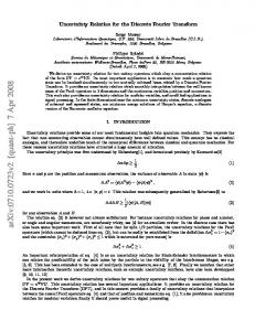
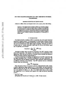
Figure 1. The diagram shows the execution of our approach. c is the chunk size that the M · N image is split into. The last step is optional and shows the FFT with the lowest frequency coefficients in the center.
x=0
Using this scheme, the computational complexity is O(N · M · log(N · M )) for the input size of N · M . IV. O UR A PPROACH This section describes the algorithm proposed in this paper. For transforming data memory efficiently into the Fourier domain we use three properties: First, we exploit the Hermite property of the transform so that no redundant values are computed. This reduces the output from N · M to ( N2 + 1) · M for data of size N · M . Secondly, we use an in-place operation for storing the computed Fourier coefficients. These two options are implemented in many DFT libraries, including the NVIDIA CUFFT Library and FFTW we use in this case. Thirdly, we reduce the size of the buffers needed for interim results as we exploit the separation of the Fourier transform. These buffers are created during the planing state of CUFFT or FFTW and are called plans. The number of lines that are transformed in parallel can be adjusted dynamically to utilize the whole device memory. Thus, there is no need to create a buffer for the whole image at once which might not fit into the memory of the device. Therefore, our approach transforms only a number of lines in parallel until all lines of the first dimension are processed and then transforms the second dimension in the same way. The final result is mathematically equal to the standard twodimensional approach. A. Algorithm The general algorithm we propose in this paper is outlined in Figure 1 and Algorithm 2. First, the original data is loaded and then transferred onto the device. There, the first dimension is transformed in portions of M c chunks. When all rows are transformed, the result is transposed and the second dimension is transformed in the same way. Afterwards, the
data is transformed back and the result is equal to a simple, but more memory consuming, fft2d call. The transposition of the data is necessary, since the DFT functions do not work on input that is stridden or padded. When the second dimension is to be transformed, its elements don’t appear in consecutive order. The transposition reorders the data and the one-dimensional transforms can be applied. For efficiency, the last transposition can be avoided, if the subsequent algorithms are aware of this, as it is just a reordering of the data. B. Optimizations Basically, the separation of the transform can be implemented in two different ways: Having all the input and output on the device, so all the computations and transpositions are done on the GPU. This approach is called “deviceonly” below. The GPU memory requirements can be further reduced by having the input and output residing on the host side and copying the chunks to the device individually, transform them there and copy them back. The transposition is done on the host side. Here, only one chunk and the buffer for its intermediate results need to fit into the GPU memory at a time. We call this version “partial copy”. On a more detailed view, the question arises, where and when the plans should be created. Calling the planning function before a transformation might result in smaller plans as the second one is also in memory. This introduces the overhead of calling the one-dimensional transforms more often because they are “smaller”. On the other hand, deleting unused plans and buffers and creating new plans on demand during the transform has the overhead of doing the same work more often when the transformation is to be applied more than once on different data. For evaluation, we used the first method and create the plans before the computation is started as previous investigations have shown that the
Algorithm 2 Lines 4 to 15 show the code corresponding to the device-only version and lines 17 to 30 show the partialcopy code. The colors and labels correspond to Figure 3. 1: cuda malloc(); 2: cufft plan(); 3: if DeviceOnly then 4: memcpyHostToDev(); 5: for i = 0; i < height; i += chunksize do 6: cufft1d(); {first dimension} 7: end for 8: transpose(); 9: for i = 0; i < width; i += chunksize do 10: cufft1d(); {second dimension} 11: end for 12: transpose(); 13: memcpyDevToHost(); 14: else 15: for i = 0; i < height; i += chunksize do 16: memcpyHostToDevChunked(); 17: cufft1d(); {first dimension} 18: transpose(); 19: memcpyDevToHostChunked(); 20: end for 21: for i = 0; i < width; i += chunksize do 22: memcpyHostToDevChunked(); 23: cufft1d(); {second dimension} 24: transpose(); 25: memcpyDevToHostChunked(); 26: end for 27: end if 28: cuda free(); {clean up} 29: cufft destroy();
plan creation is slower than the overhead of calling multiple kernels. V. R ESULTS A. Evaluation System For evaluating the following results a standard desktop PC was used. It was running Windows 7, the NVIDIA Graphics Driver 190.38 with CUDA 2.3 and driver version 190.89 with OpenCL. The processor is an Intel i7 940 running at 2,93 GHz. It has four physical cores with Hyper Threading enabled. The graphics card used is a NVIDIA GTX 285 with 1 GB device memory. B. Data sizes In the evaluation, we used a large set of different problem sizes. Power-of-2 examples are used as well as typical image resolutions. Table I shows the evaluated data set sizes and the memory needed to store the input, intermediate and output buffers by the evaluated libraries in detail.
The minimum values refer to our device-only approach since the minimum values of the partial-copy approach need only a few hundred kilobytes as we only process one column or row at a time on the device. The maximum values refer to the partial-copy and the device-only approach as the memory consumption is identical. Both methods have input and output allocated on the device and the plans are one chunk per dimension, only. The values measured directly after the plan creation show, size that CUFFT needs about four ( M ·N ≈ 16 = 4 Floats) times the space of the input for its intermediate results for the realto-complex transforms when transforming two-dimensional data. For power-of-2 one-dimensional transforms, CUFFT does not allocate memory in its planning state at all. This explains why large input dimensions do not necessarily lead to a larger memory consumption in our approach. The values in Table I are calculated as follows: N + 1) · M · C + p(N, M ) 2 sizeopencl = 2 · N · M · C N sizemin = 2 ∗ ( + 1) · M ∗ C + 2 p(N, 1) + p(M, 1) N sizemax = 2 ∗ 2 ∗ ( + 1) · M ∗ C + 2 N p(N, M ) + p(M, + 1), 2 with N being the width and M the height of the input image. C denotes sizeof(complex) which is 8 Bytes. p represents for the planning function of CUFFT and we estimated it as p(m, n) = 16 · n · m according to our measurements. sizeopencl was derived from the source code of the library. In theory, our partial-copy approach ends when one line and its according plan do not fit into memory any longer. Even in this case, the one dimensional transform could be separated and calculated in chunks, e.g. by the Cooley-Tukey approach. The following list gives an overview of the algorithms evaluated: FFTW: CPU reference implementation. It uses a precreated plan (FFTW_MEASURE flag) and eight threads. CUFFT: In-place transform of cufft2d. Neither the plan creation nor the transfer are included in the result. Our approach, device-only: The plans are pre-computed and the complete computation is done on the device. For the transposition we used the respective example included in the NVIDIA CUDA SDK3 . Our approach, partial-copy: This approach copies every data chunk to the device, transforms and transposes it there and copies it back to the host. Thus, it does not require sizecuf f t
=
(
3 http://developer.nvidia.com/object/cuda
2 3 downloads.html
Width 16384 16384 16384 16384 8192 8192 8192 6048 4096 4752 3456 2560 2048 2353 1920 1280 512
Dimensions Height MegaPixel 8192 128 7168 112 6144 96 5120 80 8192 64 6144 48 4096 32 4032 23 4096 16 3168 14 2304 8 1920 5 2048 4 1568 3 1080 2 1024 1 512 0.25
Libraries CUFFT OpenCL (2560) (2240) (1920) (1600) (1280) (960) 640 465 320 287 152 94 48 70 40 25 1
2048 – – – 1024 – 512 – 256 – – – 64 – – – 4
Our approach Min Max 1024 896 768 640 512 384 256 186 128 115 61 38 32 28 16 10 2
1024 1792 1536 1280 512 768 256 744 128 460 243 150 32 113 48 30 2
Table I Problem sizes and memory consumption of the evaluated GPU algorithms. The values in brackets are estimated as there was not enough memory on the device. The values are rounded to full Megapixel and Megabytes, respectively. We calculate the Megapixel by W idth·Height . 1024·1024
the complete input and output to be located on the device and can be used when there is not enough device memory available. OpenCL: Apples sample for DFT using OpenCL. C. NVIDIA CUFFT Library The NVIDIA CUFFT Library is a closed source Library providing DFT algorithms for CUDA enabled graphics cards. It uses a planning interface which allocates the buffers for intermediate results and some functions for transforming one-, two- and three-dimensional data forward and backward. As far as memory consumption is concerned, the CUFFT uses a very high amount of memory (see Table I). To save some memory when using CUFFT, we use the in-place transform which overwrites the input during the transformation. When comparing this to the out-of-place transform, there is no measurable difference in execution time. The one-dimensional DFT function of CUFFT has a parameter for so called batch transforms. This option allows to apply the transformation to more than one line at a time and thus saves GPU kernel calls. However, the parameter also influences the size of the buffer allocated by CUFFT linearly. It allows to trade memory consumption for execution time. D. FFTW The libfftw3 (version 3.2.2) library is an open source project implementing the DFT for various platforms. Its aim is to have a very fast implementation and it uses an offline planning function for finding the optimal calculation pattern. This chosen mode FFTW_MEASURE has a time consuming
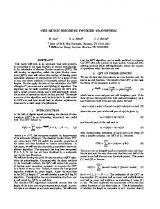
planning phase. It tries different methods for decomposing the transform and selects the fastest one for the actual transformation. The FFTW scales well with multiple cores. We used eight threads in our evaluation. E. OpenCL We also used the DFT example by Apple for comparing its performance with CUFFT and our approach. As it is only able to handle problem sizes of power-of-2 and has huge CPU memory requirements, we were only able to run it up to 16 Megapixel (32bit executable). F. Discussion of the Results Figure 2 shows the results of our experiments. The peak at 3.52 Megapixel, which affects all implementations of the DFT, is a result of the “Fourier-unfriendly” size of 2353 · 1568 (its prime factors are 13 and 181). The first dimension is not nicely separable and thus all implementations need significantly more time for processing it than for a size with smaller prime factors. In this case, it would be beneficial to pad the image as even the 8 Megapixel image transforms faster if it already resides on the GPU. For small images (up to 4 Megapixel), NVIDIA’s CUFFT implementation is faster than our device-only approach. For larger images (starting at around 4 Megapixel), our approach runs faster. As our approach targets setups in which only a low amount of memory is available for DFTs, we ran a second benchmark on the same hardware but with 500 Megabytes of memory allocated previously. When dealing with lower sized data, the measurements are exactly the same as presented in Figure 2 since there is enough memory and the configurations work the same way. Starting from 16 Megapixel, the CUFFT library is not able to compute the Fourier coefficients anymore because there is not enough memory for the plans and the intermediate results. 48 Megapixel is the biggest amount of data which our device-only approach can handle. Hence, only our partial-copy approach is able to run on the GPU. In Figure 3, we present a more detailed view on a selection of the evaluated algorithms. The timings are separated into the important steps and measured accurately using the CudaEvent API. Those timers measure the GPU time of the kernel called which is normally asynchronous to the host and thus nearly transparent to the host timers. What can be seen is that most of the time of the device-only approach is spent in the transform. Note, that the second dimension only has N2 + 1 complex rows to transform and thus is faster than M transforms of the first dimension. For the partialcopy approach, the same time is spent there plus the cost for the memory operations. Comparing it to CUFFT, the OpenCL approach is slightly slower and at 16 Megapixels even slower than the FFTW on
FFTW
CUFFT
OpenCL
device-only
partial-copy
Time [Milliseconds]
150
100
50
0 0.25
2
34 5
8
15
16
23
32
Data Size [Megapixel]
Time [Seconds]
800
600
400
200
0
16
23
32
48
64
80
96
112
128
Data Size [Megapixel]
Figure 2. Both graphs show the same measurements. The upper graph has a closer look on the lower values. The lower graph provides an overview of the image size starting at 16 Megapixel. For CUFFT and our device-only approach, dashed lines show where they were able to perform when there were 1024 Megabytes available. With 500 Megabytes preallocated, they are only able to handle the values along the solid line. Red numbers are power of 2
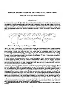
the CPU. Since it only does complex-to-complex transforms, the comparison is only exemplary. Figure 4 shows the performance of our partial-copy algorithm according to the memory it uses. The chunk size was selected for these measurements (noted on the upper x axis of the figure). The performance is shown in comparison to the run with all memory available, falling down to 4% of its original speed for a chunk size of 2. What can be seen is that the performance starts to drop drastically at a
chunk size below 100, still having about 72% of the original performance for memory usage of about 5% (according to the chunk size of 128 (40 Megabytes memory usage) and the maximum memory usage of about 744 Megabytes). At this point, the number of kernel calls is 316. VI. C ONCLUSION & F UTURE W ORK In this paper we presented an approach for using existing DFT libraries in a memory saving way. We use the sepa-
FFT Device to Host
Host to Device Transpose FFTW
The presented technique could be integrated in existing GPU DFT libraries to trade-off memory and computation time. Furthermore, it increases the maximum image size which can be processed significantly.
89.7
CUFFT
R EFERENCES
64.0
[1] NVIDIA, “CUDA CUFFT Library,” 2010.
part-cpy
134.4
dev-only
46.0 0
50
100
150
Time [ms] Figure 3. Detailed timing measurements of our approaches. The values are taken from the 23.26 Megapixel example on the full memory configuration. For the partial-copy approach, all four stages are shown. The chunk size was 2125 for the first and 1594 for the second dimension. The colors and labels correspond to Algorithm 2.
Chunksize 512 256 128
64 32 16
8
4
2
100%
10000
75%
1000
50%
100
25%
Kernel Calls
1/Factor
Max
10 0 Max
183 87 40 15 8 4 2 1 0.5 Memory Usage [Megabytes]
Figure 4. Performance (squares) and number of kernel calls (circles) of our partial-copy approach compared to its memory usage. The problem size used for evaluation was the 23 Megapixel image. Note that the x axes and right y axis are scaled logarithmically.
rability of the Fourier transform to compute only parts of the coefficients at a time using the available memory. Our approach has been implemented using CUDA and CUFFT which is very memory consuming by default. Evaluating the results has shown that our approach is faster than CUFFT for data sizes starting at about 4 Megapixel, even though we use functions provided by CUFFT and NVIDIA. For larger images, which cannot be processed entirely on the device due to memory constraints, we provide a method that does the transformation on the GPU and the transposition on the CPU. The approach we presented in this paper was evaluated only for two dimensional problems, but it can be applied for higher dimensional transforms as well. This could be useful for medical or geological data sets where three dimensional arrays need to be transformed.
[2] M. Frigo and S. G. Johnson, “The design and implementation of FFTW3,” Proceedings of the IEEE, vol. 93, no. 2, pp. 216–231, 2005, special issue on “Program Generation, Optimization, and Platform Adaptation”. [3] M. Frigo and S. Johnson, “FFTW: An adaptive software architecture for the FFT,” Acoustics, Speech and Signal Processing, 1998. Proceedings of the 1998 IEEE International Conference, vol. 3, pp. 1381–1384, May 1998. [4] O. Fialka and M. Cadik, “FFT and convolution performance in image filtering on GPU,” in Information Visualization, 2006. IV 2006. Tenth International Conference on, July 2006, pp. 609–614. [5] K. Moreland and E. Angel, “The FFT on a GPU,” in HWWS ’03: Proceedings of the ACM SIGGRAPH/EUROGRAPHICS conference on Graphics hardware. Aire-la-Ville, Switzerland, Switzerland: Eurographics Association, 2003, pp. 112– 119. [6] N. K. Govindaraju, B. Lloyd, Y. Dotsenko, B. Smith, and J. Manferdelli, “High performance Discrete Fourier Transforms on graphics processors,” Microsoft. [7] T. G. Stockham, Jr., “High-speed convolution and correlation,” in AFIPS ’66 (Spring): Proceedings of the April 26-28, 1966, Spring joint computer conference. New York, NY, USA: ACM, 1966, pp. 229–233. [8] V. Volkov and B. Kazian, “Fitting FFT onto the G80 architecture,” University of California, Berkeley, 2008. [9] R. Bracewell and P. B. Kahn, “The Fourier transform and its applications,” American Journal of Physics, vol. 34, no. 8, pp. 712–712, 1966. [Online]. Available: http: //link.aip.org/link/?AJP/34/712/3 [10] J. K. Sanjit K. Mitra and K. Sanjit, Handbook for Digital Signal Processing. John Wiley & Sons, 1993. [11] J. O. Smith, Mathematics of the Discrete Fourier Transform (DFT). http://ccrma.stanford.edu/ jos/mdft/, February, 2010 (date accessed), online book.