MemTri: A Memory Forensics Triage Tool using Bayesian Network and ...

MemTri: A Memory Forensics Triage Tool using Bayesian Network and Volatility

Rohan Murray Department of Computer Science University of Westminster

A Dissertation Submitted to the Department of Computer Science in Partial Fulfillment of the Requirements for the Cyber Security and Forensics MSc London, UK, 2016

Academic Supervisor: Dr. Antonis Michalas, University of Westminster Day of the defence: September 19, 2016 Submitted Date: September 14, 2016

ii

c

Copyright by ROHAN MURRAY. All rights reserved.

“For everyone practicing evil hates the light and does not come to the light, lest his deeds should be exposed.“ John 3:20 NKJV

iii

Abstract In this modern era of technology, it is becoming more common for digital devices to be seized as evidence. This has lead to a backlog of digital evidence to be analysed for court cases. A proposed solution to this ’data volume challenge’ is to develop digital forensics triage tool that utilises data mining techniques such as supervised machine learning. Apparently, no research has yet been published for the development of a memory forensics triage tools capable of performing crime classification of a memory image. This work explores the development of such a memory forensics triage tool, labelled MemTri, that can assess the likelihood of criminal activity in a memory image, based on evidence data artefacts generated by several applications. Fictitious illegal firearms suspect activity scenarios were performed on virtual machines to generate 60 test memory images for input into MemTri. Four categories of applications (i.e. Internet Browsers, Instant Messengers, FTP Client and Document Processors) are examined for data artefacts located through the use of regular expressions. These identified data artefacts are then analysed using a Bayesian Network, to assess the likelihood that a seized memory image contained evidence of illegal firearms trading activity. MemTri’s normal mode of operation achieved a high artefact identification accuracy performance of 95.7% when the applications’ processes were running, however this fell significantly to 60% as applications processes’ were terminated. To explore improving MemTri’s accuracy performance, a second (scan) mode was developed, which achieved more stable results of around 80% accuracy, even after applications processes’ were terminated.

Acknowledgements This dissertation could not have been completed without the support of various individuals. I would therefore like to express my appreciation to: • My loving Creator, who set in place all that I needed to complete this project, while inspiring me with written words of wisdom and assurance. • My fiance, who offered consistent emotional support, took the time to listen to my analytical ramblings and proofread my dissertation. • My father and mother for their prayers and encouragement. • My supervisor for his constant encouragement and guidance. • The University of Westminster technical support team for assisting in preparation of the computer laboratory for me to successfully perform my experiments. • The participants that responded to the online memory forensics questionnaire, whoever you are!

List of Figures 3.1 3.2 3.3 3.4

Bayesian Bayesian Bayesian Bayesian

. . . .

. . . .

14 19 22 25

4.1 4.2 4.3 4.4 4.5 4.6

. . . . .

27 30 31 32 33

4.16

Physical Layout of a modern computer system [1] . . . . . . . . . Segmentation and Paging Process [2] . . . . . . . . . . . . . . . . Translation of Logical Address to Linear Address [2] . . . . . . . Virtual Memory Address for 4MB page size . . . . . . . . . . . . Virtual Memory Address for 4KB page size . . . . . . . . . . . . Translation of Virtual Address to Physical Address for 4KB page size [2] . . . . . . . . . . . . . . . . . . . . . . . . . . . . . . . . . Combination of base address in CR3 register with Directory offset in VA to produce the PDE Address . . . . . . . . . . . . . . . . . Combination of base address in PDE with Page Table offset in VA to produce the PTE Address . . . . . . . . . . . . . . . . . . . . Combination of base address in PTE and with Page Frame offset in VA to produce the Physical Address . . . . . . . . . . . . . . . Basic Resources of a Process [1] . . . . . . . . . . . . . . . . . . . Diagram showing how an Object is referenced in the Object table of a Process [1] . . . . . . . . . . . . . . . . . . . . . . . . . . . . Diagram showing shared and independent resources of Process and Threads [3] . . . . . . . . . . . . . . . . . . . . . . . . . . . . . . Process’ virtual address space and stored resource areas [1] . . . DKOM attack on EPROCESS structure to hide a process [4] . . . Simple dd command to collect memory from Windows physical memory object device . . . . . . . . . . . . . . . . . . . . . . . . Suspended VMware virtual machine’s memory in .vmem file . . .

6.1 6.2

Designed steps for MemTri’s Evidence Search Engine component . 64 Designed Bayesian Network Model for the MemTri Application . . 66

7.1

Program flowchart for MemTri application. Green shapes are ESE related process; Purple shapes are BNA related processes . . . . . 69

4.7 4.8 4.9 4.10 4.11 4.12 4.13 4.14 4.15

Network Network Network Network

Connections . . . . . . . . . . . . Inference Diagram . . . . . . . . . Example . . . . . . . . . . . . . . with Observed Evidence Example

i

. . . .

. . . .

. . . .

. . . .

. . . .

. . . .

. 33 . 33 . 34 . 34 . 36 . 38 . 39 . 40 . 42 . 47 . 49

LIST OF FIGURES

7.2 7.3

Example of Google search data artefact identified with a ‘strong’ regular expression . . . . . . . . . . . . . . . . . . . . . . . . . . . 73 Example of File Open/Save data artefact identified with a ‘weak’ regular expression . . . . . . . . . . . . . . . . . . . . . . . . . . . 73

8.1

MemTri’s average accuracy results for executions in normal and scan mode across the three phase sets of test images . . . . . . . . 8.2 MemTri’s average precision results for executions in normal and scan mode across the three phase sets of test images . . . . . . . . 8.3 MemTri’s average recall results for executions in normal and scan mode across the three sets of phase test images . . . . . . . . . . . 8.4 Volatility’s ’pslist’ plug-in output for image #29 showing chrome.exe process marked as terminated immediately after application was exited . . . . . . . . . . . . . . . . . . . . . . . . . . . . . . . . . . 8.5 MemTri’s average f-measure results for executions in normal and scan mode across the three sets of phase test images . . . . . . . . 8.6 Average ’Yes’ Likelihood that a specific application type was used to commit illegal firearms trading based on Question 4 results of the Digital Forensics Expert Questionnaire . . . . . . . . . . . . . 8.7 The projected ranking for each experiment performed in reference to the total number of scenarios performed . . . . . . . . . . . . . 8.8 Standard deviation of MemTri’s normal and scan mode ranking results for the three phase sets of test images . . . . . . . . . . . . 8.9 Average likelihood of finding evidence artefacts for the various application types based on expert questionnaire responses to Questions 4–8 . . . . . . . . . . . . . . . . . . . . . . . . . . . . . . . . . 8.10 Example of an irrelevant case evidence artefact identified by MemTri for scenario id D1 of image #11 . . . . . . . . . . . . . . . . . . .

80 81 83

84 85

87 88 89

91 92

A.1 Format of the CR3 and Paging-Structure Entries for 32-Bit Paging [2]108 B.1 Overview of the Windows OS Architecture [5] . . . . . . . . . . . . 109 C.1 List of Windows Executive Objects [1] . . . . . . . . . . . . . . . . 110

ii

List of Tables 3.1 3.2 3.3

Likelihood Joint Probability Table for P(H1 | H) . . . . . . . . . . 23 Likelihood Joint Probability Table for P(E1 | H1) . . . . . . . . . 23 Likelihood Joint Probability Table for P(E2 | H1) . . . . . . . . . 24

4.1

Volatility’s volshell command output for the EPROCESS structure . 37

6.1 6.2 6.3

List of applications installed by type . . . . . . . . . . . . . . . . . 61 List of suspect activity scenarios developed . . . . . . . . . . . . . 62 Symbolised meaning of the nodes in MemTri’s BNM; IBE*-Internet Browser Evidence, IME*-Instant Messenger Evidence, DPE*-Document Processor Evidence, FTPE*-FTP Client Evidence . . . . . . . . . 66

7.1 7.2

Template for inserting Joint Probability Table values . . . . . . . . 77 Example of Joint Probability Tables values for P (H1 |H) . . . . . . 77

8.1

Matrix of performance measurement variables used to calculate accuracy, precision and recall. . . . . . . . . . . . . . . . . . . . . . 79 Projected Ranking of Test Image experiments based on expert knowledge questionnaire results encoded into BNA . . . . . . . . . 88 Standard deviations between MemTri’s test image ranking results and the ideal projected ranking . . . . . . . . . . . . . . . . . . . . 89

8.2 8.3

G.1 Template for collecting test images based on experiments involving multiple scenario ids . . . . . . . . . . . . . . . . . . . . . . . . . . 122 H.1 Example of Data Artefacts matched by the Regular Expressions in the evidence search engine.cpp . . . . . . . . . . . . . . . . . . . 124 I.1

Lines in the evidence search engine.cpp file where the Regular Expressions are implemented . . . . . . . . . . . . . . . . . . . . . . . 126

J.1

Scenarios Found results for MemTri’s Normal Mode execution on Running Phase test images . . . . . . . . . . . . . . . . . . . . . . 128 Scenarios Found results for MemTri’s Scan Mode execution on Running Phase test images . . . . . . . . . . . . . . . . . . . . . . . . . 129

J.2

iii

LIST OF TABLES

J.3 J.4 J.5 J.6

Scenarios Found results for MemTri’s Normal Mode execution on Stopped Phase test images . . . . . . . . . . . . . . . . . . . . . . Scenarios Found results for MemTri’s Scan Mode execution on Stopped Phase test images . . . . . . . . . . . . . . . . . . . . . . Scenarios Found results for MemTri’s Normal Mode execution on Delayed Phase test images . . . . . . . . . . . . . . . . . . . . . . Scenarios Found results for MemTri’s Scan Mode execution on Delayed Phase test images . . . . . . . . . . . . . . . . . . . . . . .

. 130 . 131 . 132 . 133

K.1 Performance Results for MemTri’s Normal Mode execution on Running Phase test images. Note duration in seconds . . . . . . . . . . 135 K.2 Performance Results for MemTri’s Scan Mode execution on Running Phase test images. Note duration in seconds . . . . . . . . . . 136 K.3 Performance Results for MemTri’s Normal Mode execution on Stopped Phase test images. Note duration in seconds . . . . . . . . . . . . . 137 K.4 Performance Results for MemTri’s Scan Mode execution on Stopped Phase test images. Note duration in seconds . . . . . . . . . . . . . 138 K.5 Performance Results for MemTri’s Normal Mode execution on Delayed Phase test images. Note duration in seconds . . . . . . . . . 139 K.6 Performance Results for MemTri’s Scan Mode execution on Delayed Phase test images. Note duration in seconds . . . . . . . . . 140 L.1 Output Rating Results for MemTri’s Normal Mode execution on Running Phase test images. . . . . . . . . . . . . . . . . . . . . . . 142 L.2 Output Rating Results for MemTri’s Scan Mode execution on Running Phase test images. . . . . . . . . . . . . . . . . . . . . . . . . 143 L.3 Output Rating Results for MemTri’s Normal Mode execution on Stopped Phase test images. . . . . . . . . . . . . . . . . . . . . . . 144 L.4 Output Rating Results for MemTri’s Scan Mode execution on Stopped Phase test images. . . . . . . . . . . . . . . . . . . . . . . . . . . . 145 L.5 Output Rating Results for MemTri’s Normal Mode execution on Delayed Phase test images. . . . . . . . . . . . . . . . . . . . . . . 146 L.6 Output Rating Results for MemTri’s Scan Mode execution on Delayed Phase test images. . . . . . . . . . . . . . . . . . . . . . . . . 147 M.1 Data Collected from Digital Forensics Expert Questionnaire; VL*=Very Likely, L*=Likely, ALAN=As Likely As Not, UL*=Unlikely, VUL=Very Unlikely, Unc.=Uncertain, W. Avg.= Likelihood Weighted Average 148

iv

Contents List of Figures

i

List of Tables

iii

1 Introduction 1.1 Motivation . . . . . . . . . . . . . . . 1.2 Aims and Objectives . . . . . . . . . . 1.2.1 Aims . . . . . . . . . . . . . . . 1.2.2 Objectives . . . . . . . . . . . . 1.3 Contributions . . . . . . . . . . . . . . 1.3.1 Memory Artefact Identification 1.3.2 Expert Knowledge Collection . 1.3.3 Memory Forensics Triage . . . 1.4 Outline . . . . . . . . . . . . . . . . .

. . . . . . . . .

. . . . . . . . .

. . . . . . . . .

. . . . . . . . .

. . . . . . . . .

. . . . . . . . .

. . . . . . . . .

. . . . . . . . .

. . . . . . . . .

. . . . . . . . .

. . . . . . . . .

. . . . . . . . .

. . . . . . . . .

. . . . . . . . .

. . . . . . . . .

. . . . . . . . .

1 1 3 3 4 5 5 5 5 6

2 Preliminaries 8 2.1 Memory Forensics . . . . . . . . . . . . . . . . . . . . . . . . . . . 8 2.2 Bayesian Network . . . . . . . . . . . . . . . . . . . . . . . . . . . . 10 3 Bayesian Network 3.1 Bayes’ Theorem . . . . . . . . . . . . . . . . . . . . . . . . 3.1.1 Bayes’ Theorem and Digital Forensics . . . . . . . 3.2 Bayesian Probability . . . . . . . . . . . . . . . . . . . . . 3.2.1 Conditional Probability . . . . . . . . . . . . . . . 3.2.2 Derivation of Bayes’ Theorem . . . . . . . . . . . . 3.3 Bayesian Network Model . . . . . . . . . . . . . . . . . . . 3.3.1 Conditional Independence . . . . . . . . . . . . . . 3.3.1.1 Casual Chain . . . . . . . . . . . . . . . . 3.3.1.2 Common Cause . . . . . . . . . . . . . . 3.3.1.3 Common Effect . . . . . . . . . . . . . . 3.3.2 Translating Bayesian Network Model to Equations 3.3.2.1 BNM #1: Single Node . . . . . . . . . . 3.3.2.2 BNM #2: Two Node Serial Connection .

v

. . . . . . . . . . . . .

. . . . . . . . . . . . .

. . . . . . . . . . . . .

. . . . . . . . . . . . .

. . . . . . . . . . . . .

11 11 11 12 12 13 13 14 14 14 14 15 15 16

CONTENTS

3.4

3.3.2.3 BNM #3: Three Nodes Serial Connection . 3.3.2.4 BNM #4: Diverging Connection . . . . . . 3.3.2.5 BNM #5: Converging Connection . . . . . Bayesian Inference . . . . . . . . . . . . . . . . . . . . . . . 3.4.1 Calculation Methods of Bayesian Inference . . . . . 3.4.1.1 Bayesian Inference by Enumeration . . . . 3.4.1.2 Bayesian Inference by Variable Elimination 3.4.2 Bayesian Network Example . . . . . . . . . . . . . .

4 Volatile Memory 4.1 Computer Memory . . . . . . . . . . . . . . . . . . 4.2 PC Architecture . . . . . . . . . . . . . . . . . . . 4.2.1 Memory Management Unit . . . . . . . . . 4.2.2 Direct Memory Access (DMA) Controller . 4.3 CPU Architecture . . . . . . . . . . . . . . . . . . 4.3.1 Registers . . . . . . . . . . . . . . . . . . . 4.3.2 Cache . . . . . . . . . . . . . . . . . . . . . 4.4 Memory Management . . . . . . . . . . . . . . . . 4.4.1 Segmentation . . . . . . . . . . . . . . . . . 4.4.2 Paging . . . . . . . . . . . . . . . . . . . . . 4.4.2.1 Page Address Translation . . . . . 4.5 Windows Operating System Process . . . . . . . . 4.5.1 Windows OS Architecture . . . . . . . . . . 4.5.2 Windows Process Structure and Resources . 4.5.2.1 Windows Process Object . . . . . 4.5.2.2 Handles . . . . . . . . . . . . . . . 4.5.2.3 Tokens: Security Access . . . . . . 4.5.2.4 Threads . . . . . . . . . . . . . . . 4.5.2.5 Virtual Address Descriptors . . . 4.5.2.6 Process Environment Block . . . . 4.5.3 Enumerating Windows Processes . . . . . . 4.6 Memory Acquisition . . . . . . . . . . . . . . . . . 4.6.1 Hardware-based Methods . . . . . . . . . . 4.6.1.1 DMA Attack . . . . . . . . . . . . 4.6.1.2 Cold Boot Attack . . . . . . . . . 4.6.2 Software-based Methods . . . . . . . . . . . 4.6.2.1 Kernel-Level Acquisition . . . . . 4.6.2.2 User-Level Acquisition . . . . . . . 4.6.2.3 Virtualisation Acquisition . . . . .

. . . . . . . . . . . . . . . . . . . . . . . . . . . . .

. . . . . . . . . . . . . . . . . . . . . . . . . . . . .

. . . . . . . . . . . . . . . . . . . . . . . . . . . . .

. . . . . . . . . . . . . . . . . . . . . . . . . . . . .

. . . . . . . . . . . . . . . . . . . . . . . . . . . . .

. . . . . . . .

. . . . . . . .

. . . . . . . .

. . . . . . . .

16 17 17 18 18 19 20 21

. . . . . . . . . . . . . . . . . . . . . . . . . . . . .

. . . . . . . . . . . . . . . . . . . . . . . . . . . . .

. . . . . . . . . . . . . . . . . . . . . . . . . . . . .

. . . . . . . . . . . . . . . . . . . . . . . . . . . . .

26 26 27 27 28 28 28 29 30 31 31 33 34 35 35 36 37 38 38 39 41 41 43 43 44 45 47 47 48 48

5 Background & Related Work 50 5.1 Source of the Problem . . . . . . . . . . . . . . . . . . . . . . . . . 50 5.2 Digital Forensics and Triage Solutions . . . . . . . . . . . . . . . . 50 5.3 Data-mining and Digital Forensics Triage . . . . . . . . . . . . . . 52

vi

CONTENTS

5.4

5.5 5.6 5.7

DFT with Supervised Machine Learning . . . . . . . 5.4.1 Support Vector Machines . . . . . . . . . . . 5.4.2 Decision Trees . . . . . . . . . . . . . . . . . 5.4.3 K-Nearest Neighbour . . . . . . . . . . . . . . 5.4.4 Bayesian Network . . . . . . . . . . . . . . . 5.4.5 General Limitation of applying SML in DFT Extraction of Data Artefacts . . . . . . . . . . . . . Data Artefact Feature Translation . . . . . . . . . . Concluding Note . . . . . . . . . . . . . . . . . . . .

6 Design and Methodology 6.1 Suspect Machine Preparation . . . 6.2 Suspect Activity Scenarios . . . . . 6.3 Memtri Application Design . . . . 6.3.1 Evidence Search Engine . . 6.3.2 Bayesian Network Analyser

. . . . .

. . . . .

. . . . .

. . . . .

. . . . .

. . . . .

. . . . .

. . . . .

. . . . .

. . . . .

. . . . . . . . .

. . . . . . . . .

. . . . . . . . .

. . . . . . . . .

. . . . . . . . .

. . . . . . . . .

. . . . . . . . .

. . . . . . . . .

53 53 54 54 55 57 57 58 59

. . . . .

. . . . .

. . . . .

. . . . .

. . . . .

. . . . .

. . . . .

. . . . .

60 60 61 63 63 64

. . . . . . . . . . . . .

67 67 67 68 68 70 70 71 71 72 74 75 75 76

. . . . . . . . . . .

78 78 79 81 82 85 86 86 90 90 91 92

7 Implementation 7.1 Collection of the Memory Images . . . . . . . . . . . . . . . 7.1.1 Generating the Training Memory Images . . . . . . 7.1.2 Generating the Test Memory Images . . . . . . . . . 7.2 MemTri Application Development . . . . . . . . . . . . . . 7.2.1 Modes of Operation . . . . . . . . . . . . . . . . . . 7.2.2 Evidence Search Engine Implementation . . . . . . . 7.2.2.1 Locating the Target Application Processes 7.2.2.2 Extracting ASCII and Unicode Text . . . . 7.2.2.3 Evidence Filtering and Feature Generation 7.2.3 Bayesian Network Analyser Implementation . . . . . 7.2.3.1 Building the Bayesian Network Model . . . 7.2.3.2 Joint Probability Tables Setup . . . . . . . 7.2.3.3 Bayesian Inference on Evidence . . . . . . . 8 Results and Evaluation 8.1 Performance . . . . . . . . . . . . . . . . . . 8.1.1 Accuracy . . . . . . . . . . . . . . . 8.1.2 Precision . . . . . . . . . . . . . . . 8.1.3 Recall . . . . . . . . . . . . . . . . . 8.1.4 F-Measure . . . . . . . . . . . . . . . 8.1.5 Overall Performance . . . . . . . . . 8.2 Output Rating . . . . . . . . . . . . . . . . 8.3 Observation and Anomalies . . . . . . . . . 8.3.1 Cross Application Memory Content 8.3.2 Concentration of Evidence Artefacts 8.3.3 Irrelevant Memory Artefacts . . . .

vii

. . . . . . . . . . .

. . . . . . . . . . .

. . . . . . . . . . .

. . . . . . . . . . .

. . . . . . . . . . .

. . . . . . . . . . .

. . . . . . . . . . .

. . . . . . . . . . .

. . . . . . . . . . .

. . . . . . . . . . . . .

. . . . . . . . . . .

. . . . . . . . . . . . .

. . . . . . . . . . .

. . . . . . . . . . . . .

. . . . . . . . . . .

CONTENTS

9 Conclusions & Future Work 93 9.1 Challenges and Limitations . . . . . . . . . . . . . . . . . . . . . . 94 9.2 Future Work . . . . . . . . . . . . . . . . . . . . . . . . . . . . . . 95 9.3 Critical Evaluation . . . . . . . . . . . . . . . . . . . . . . . . . . . 96 References

100

Appendices

108

A CR3 and Paging-Structure Entries

108

B Windows OS Architecture

109

C Windows OS Objects

110

D Case Database Files D.1 Trigger Words.txt . D.2 Context Words.txt . D.3 Flagged Websites.txt D.4 Flagged Contacts.txt D.5 Download Links.txt

. . . . .

. . . . .

. . . . .

. . . . .

. . . . .

. . . . .

. . . . .

. . . . .

. . . . .

. . . . .

. . . . .

. . . . .

. . . . .

. . . . .

. . . . .

. . . . .

. . . . .

. . . . .

. . . . .

. . . . .

. . . . .

. . . . .

. . . . .

111 111 111 112 112 112

E SASs Performance Template E.1 Internet Browser . . . . . . E.2 Instant Messenger . . . . . E.3 Document Processor . . . . E.4 FTP Client . . . . . . . . .

. . . .

. . . .

. . . .

. . . .

. . . .

. . . .

. . . .

. . . .

. . . .

. . . .

. . . .

. . . .

. . . .

. . . .

. . . .

. . . .

. . . .

. . . .

. . . .

. . . .

. . . .

. . . .

113 113 113 114 114

. . . . .

. . . . .

. . . . .

F Memory Forensics Expert Questionnaire

115

G Template for generating Test Images

121

H Sample Regular Expressions & Data Artefacts

123

I

125

Lines in MemTri’s code containing the Regular Expressions

J Results of Scenarios Found J.1 Scenarios Found Results for J.2 Scenarios Found Results for J.3 Scenarios Found Results for J.4 Scenarios Found Results for J.5 Scenarios Found Results for J.6 Scenarios Found Results for

Running Phase: Normal Mode Running Phase: Scan Mode . . Stopped Phase: Normal Mode Stopped Phase: Scan Mode . . Delayed Phase: Normal Mode . Delayed Phase: Scan Mode . .

viii

. . . . . .

. . . . . .

. . . . . .

. . . . . .

127 128 129 130 131 132 133

CONTENTS

K Performance Results K.1 Performance Results K.2 Performance Results K.3 Performance Results K.4 Performance Results K.5 Performance Results K.6 Performance Results

for for for for for for

Running Phase: Normal Mode Running Phase: Scan Mode . . Stopped Phase: Normal Mode . Stopped Phase: Scan Mode . . Delayed Phase: Normal Mode . Delayed Phase: Scan Mode . .

. . . . . .

L Priority Rankings and Output Rating Results L.1 Output Rating Results for Running Phase: Normal Mode L.2 Output Rating Results for Running Phase: Scan Mode . . L.3 Output Rating Results for Stopped Phase: Normal Mode L.4 Output Rating Results for Stopped Phase: Scan Mode . . L.5 Output Rating Results for Delayed Phase: Normal Mode L.6 Output Rating Results for Delayed Phase: Normal Mode

. . . . . .

. . . . . .

. . . . . .

. . . . . .

. . . . . .

. . . . . .

134 135 136 137 138 139 140

. . . . . .

. . . . . .

. . . . . .

141 . 142 . 143 . 144 . 145 . 146 . 147

M Data Collected from Digital Forensics Expert Questionnaire

148

N MemTri User Manaul

149

O MemTri C++ Code O.1 List of the main functions of MemTri O.2 memtri.cpp . . . . . . . . . . . . . . O.3 evidence search engine.h . . . . . . . O.4 evidence search engine.cpp . . . . . . O.5 bayesian network anaylser.h . . . . . O.6 bayesian network anaylser.cpp . . . . O.7 auxillary.h . . . . . . . . . . . . . . . O.8 auxillary.cpp . . . . . . . . . . . . .

ix

. . . . . . . .

. . . . . . . .

. . . . . . . .

. . . . . . . .

. . . . . . . .

. . . . . . . .

. . . . . . . .

. . . . . . . .

. . . . . . . .

. . . . . . . .

. . . . . . . .

. . . . . . . .

. . . . . . . .

. . . . . . . .

. . . . . . . .

. . . . . . . .

. . . . . . . .

151 151 152 163 164 175 176 181 182

Chapter 1

Introduction This project focuses on building a memory forensics triage tool, named MemTri, that has the ability to search for evidence artefacts in a memory image, after which it provides an output rating that measures the likelihood that a suspect was engaged in a specific criminal activity. The output ratings generated by MemTri can then be assessed by a law enforcement officer to determine the best priority order for performing a full analysis on a set of seized suspect memory images. To narrow the scope, this project focuses on the identification of evidence artefacts generated by a selected set of Internet Browsers, Instant Messengers, Document Processors and FTP Client applications. Also, the memory images in this work are collected in a Windows7 environment and the evidence searched for is specifically in relation to an illegal firearms trading investigation. MemTri uses the Volatility framework [6] to navigate and interpret the Windows7 structures in the memory image, when searching for evidence artefacts. The evidence artefacts found are then analysed using a Bayesian Network which incorporates digital forensics expert’s knowledge gathered through the use of a questionnaire. After analysis of the evidence artefacts found, MemTri produces a probabilistic output rating of how relevant all the located evidence is to an illegal firearms trading investigation. The ideal reader of this dissertation is expected to have a basic knowledge of computer science concepts involving volatile memory, operating systems, discrete mathematics and supervised machine learning. There are chapters dedicated to explaining the core research areas of this project, i.e. volatile memory and Bayesian Networks, in a manner that the average reader can follow the work done in this project.

1.1

Motivation

In this modern age of technology, it is becoming more common for law enforcement personnel to encounter digital devices as part of seized evidence to be examine. These digital devices include desktops, laptops, mobile phones and tablets

1

1.1 Motivation

etc. This growing influx of seized digital devices has generated a backlog of court case evidence to be forensically examined [7]. A proposed solution for alleviating this evidence backlog is to develop triage execution tools that incorporate data mining techniques [8]. The main aim of such triage tools is to quickly assess whether a digital device contains relevant case evidence or not, and how much priority should be placed on fully analysing the device. Though there have been various research into developing crime classification triage tools for disk and mobile forensics, it appears there has not yet been any published work on the development of any such similar triage tool for memory forensics. This was a bit surprising since various research has shown that memory can contain critical evidence such as internet browsing data, network traffic, malware, passwords, cryptographic keys and decrypted content, some of which may never be stored to disk [9, 10]. A possible reason for the apparent low research in developing crime classification triage tools for memory forensics is due to the complexity in analysing operating system (OS) memory structures, which is still a fairly adolescent area of research. The open-source tools Volatility [6] and Rekall [11] have aided in simplifying the analysis of such OS memory structures by incorporating the academic research done by various authors in reverse engineering these structures. Therefore, the MemTri application developed in this project, leverages from the various research incorporated into the Volatility framework [6] in order to analyse OS memory structures. It was simply decided to utilise the Volatility framework [6] for this project, due to it being the most widely utilised and tested memory analysis tool in the academic community. Another factor that may have contributed to the apparent research in developing crime classification triage tools for memory forensics, is due to the fact that acquiring memory requires careful planning and skill in order to collect a ‘forensically sound’ [12] memory image, which in-turn has led to the slow adoption of performing memory image acquisitions by law enforcement departments. Another challenge in memory forensics is that, if the user terminates the application process used to perform an illegal activity then the freed virtual address space is often quickly overwritten by other activity within the operating system. Based on Garfinkel et al.’s [13] research however, portions of unallocated memory can remain unchanged for up to 14 days, even when the system is actively being utilised. Therefore, since some data artefacts may not be overwritten in unallocated memory space by the OS, it is still possible to extract such data artefacts for memory analysis, similar to carving for files in a file system. In this work, MemTri is developed with two modes of operation, namely normal and scan mode, that give insights for the best methods to process evidence artefacts in a volatile memory environment. The Evidence Search Engine (ESE) component of MemTri mainly uses regular expressions in order to locate evidence artefacts in memory. This approach was taken based on research done by [10, 14, 15] which showed that intuitive evidence artefacts can be retrieved by simply searching for ASCII/Unicode data patterns

2

1.2 Aims and Objectives

generated by specific applications. This regular expressions approach is also flexible in that it can locate evidence artefacts in a memory image regardless of the OS environment in which the artefacts were generated. Additionally, regular expressions can be executed fairly quickly to locate evidence within large datasets. This intuitiveness, flexibility and speed offered by regular expression evidence searching methods, are essential traits for the development of an effective digital forensics triage tool. The Bayesian Network Analyser (BNA) component of MemTri, as the name suggests, uses a Bayesian Network to analyse the evidence found by the ESE. An output rating is then produced that can be used to rank a set of suspect memory images, based on the likelihood level of criminal activity. It was decided to build the Bayesian Network based on the model proposed by Ray and Shenoi [16], since it is simple to interpret and has proven successful in correctly analysing real-life criminal investigations. Comparative studies have also analysed that Bayesian approaches to developing digital forensics triage tools, on average have the best accuracy performance [17] (88.5%) compared to other supervised machine learning (SML) techniques such as Support Vector Machines, Decision Trees and K-Nearest Neighbour. This combination of accuracy and ease of interpretation supported by Bayesian Network approaches, are favourable traits when seeking to triage a criminal investigation. Additionally, of the aforementioned SML techniques, Bayesian Networks handles missing evidence most eloquently, since it is naturally incorporated into its design. Handling missing evidence is particularly a key part of forensics investigations, since evidence can often be missing due to it being destroyed or not yet discovered.

1.2

Aims and Objectives

The following sections states the various aims and objectives set for this project to be successfully executed.

1.2.1

Aims

The main aim of this project is to quantitatively measure the likelihood that a specific criminal offence was committed, based on evidence data artefacts found in Random Access Memory (RAM), in order to determine the priority that should be placed on fully examining a set of memory images. To achieve this aim a Windows7 memory forensics triage tool named MemTri will be developed that utilises Bayesian Networks and the Volatility Framework. The secondary aim of this project involves assessing the effectiveness of locating data artefacts in RAM, after the process that generated the artefact has terminated.

3

1.2 Aims and Objectives

1.2.2

Objectives

In order for MemTri to achieve the aims of this project; the following objectives have been set. Base Objectives: 1. Build an Evidence Search Engine to extract artefacts from internet browsers, instant messengers and document processors, and link the evidence artefacts to their applications process. The final output of the Evidence Search Engine is called features. 2. Develop an Evidence Weighting System that assigns numeric weights to evidence based on the importance/value of an evidence artefact to a criminal investigation. The system should use either manually entered weights or automatically assigned weights based on heuristic rules. 3. Develop a mechanism for users to modify the keywords or patterns used to search for evidence. 4. Design a Bayesian Network Model that incorporates the knowledge of digital forensics experts about the likelihood that a specific evidence artefact, if found, has contributed to a performing a specific criminal offence. 5. Build a Bayesian Network Analyser that processes the features found in a memory image and provides a numeric Bayesian Network output rating, which is a measurement of the likelihood that a specific criminal offence was committed 6. Collect a set of training and test memory images at three different phase points; (1) while the targeted applications are running, (2) immediately after the targeted applications have been terminated and (3) Five minutes after the targeted applications have been terminated. Enhanced Objectives: 1. Build a Case Classifier that provides a numeric Bayesian Network output rating for two different kinds of criminal offences. For example, MemTri should provide an output rating for illegal firearms dealership and another output rating for illegal drugs dealership. The Digital Investigator can then compare both ratings to determine which of the two criminal offences was likely committed. 2. Upgrade the Evidence Search Engine to extract evidence artefacts from an email client and link the artefact to the applications process.

4

1.3 Contributions

3. Provide a Case Evidence Report that shows where in the memory image evidence was found, the application process associated with evidence and the total number of evidence artefacts found etc. This can help to further triage the digital investigators criminal investigation by identifying where the most relevant evidence is likely located and thus where best to begin his full memory analysis.

1.3

Contributions

The performance of this project contributes to various digital forensics research such as memory artefact identification, expert knowledge collection and Memory Forensics Triage. These contributions are expounded in the following subsections.

1.3.1

Memory Artefact Identification

This project provides regular expression patterns that can be used to identify various types of memory artefacts generated by various applications, namely, Chrome, Tor, Filezilla, Skype, Wickr, Libre Writer and Microsoft’s Notepad. This project also confirms the regular expressions patterns designed by [14, 10] to locate browser memory artefacts generated by visiting websites and performing Google search engine queries. Further research is also done in developing regular expressions that capture other kinds of browser artefacts such as those generated when a file is downloaded. Simon [15] in his research noted that Skype contact information and communication content can be extracted from physical memory, however did not provide regular expressions patterns to capture this data. Therefore, this research confirms the existence of such Skype information in memory and develops regular expressions to capture these Skype memory artefacts.

1.3.2

Expert Knowledge Collection

A demonstration is given of how to design a questionnaire using SurveyMonkey [18], that can be used to gather expert knowledge data, which is then encoded into a Bayesian Network Model. Ray and Shenoi [16] in their development of a Bayesian Network also utilised a questionnaire approach however the server that hosted the sample questionnaire is no longer available. Additionally, this work illustrates the steps taken to translate the expert knowledge from the designed SurveyMonkey questionnaire into Bayesian Network Model.

1.3.3

Memory Forensics Triage

This project presents a Memory Forensics Triage application named MemTri, that has the ability to provide an output rating which measures the likelihood level of a specific criminal activity, found within a memory image. As previously mentioned, there appears to be no published research that attempted to develop a

5

1.4 Outline

digital forensics triage tool aimed specifically at analysing criminal activity found in a memory image, using SML techniques. This work examines the effectiveness of two designed approaches for locating criminal evidence in memory. The first approach involves using Volatility [6] framework to dump the memory of target applications which are then searched for evidence. The second approach involves scanning the entire memory for evidence. Therefore, the results of this project gives insights into which of these approaches is generally better suited for a memory forensics triage environment.

1.4

Outline

The rest of this dissertation is divided into the following parts: • Chapter 2 – Preliminaries: Introduces the main areas of research utilised in the development of MemTri. • Chapter 3 – Bayesian Network: Explains what is Bayes’ Theorem and how it is utilised in the context of Digital Forensics to analyse hypotheses and evidence. Steps are also given of how to build a Bayesian Network model and the significance of the node connections based on logical reasoning. Finally, an example is used to demonstrate how statistical inference is performed within a Bayesian Network using Bayes’ Theorem. • Chapter 4 – Volatile Memory: Explain what is volatile memory and where it is located within a modern computer system. The memory management mechanisms of segmentation and paging are then discussed along with an illustration of how memory addresses are translated for both mechanisms. A close look is taken at the Windows process structure and the common data fields of forensic interest are highlighted. Finally, an analysis is made of various memory acquisition techniques in terms of the forensic quality of the images produced. • Chapter 5 – Background and Related Work: Discusses the importance of the contributions made by this project to the area of digital forensics triage. An assessment is also made of other comparative triage work done using various supervised machine learning techniques. Finally, various research to locating data artefacts in memory are discussed. • Chapter 6 – Design and Methodology: Presents the intended design for the MemTri application. An outline is given of the experiment setup and memory acquisition steps. Finally, the design details for the two main components of MemTri are explained. • Chapter 7 – Implementation: Describes how the design for MemTri was actually executed.

6

1.4 Outline

• Chapter 8 – Results and Evaluation: Presents the results from the execution of MemTri on the test images collected. An evaluation is made of the results and any interesting observations were also highlighted. • Chapter 9 – Conclusions: Summarises the work done in this project and highlights challenges and limitations that were encountered. Recommendations are also given for future work that can be undertaken. Finally, an objective assessment is given of whether the aims and objectives set for this project were achieved.

7

Chapter 2

Preliminaries This chapter gives an overview of the main areas of research covered in this project, i.e. Memory Forensics (see Chapter 4) and Bayesian Networks (see Chapter 3). The area of Memory Forensics, specifically focuses on the analysis of artefacts found in main memory i.e DRAM, while the Bayesian Network area focuses on rational decision-making based on evidence (whether present or missing) given an hypothesis. It is this extraction of artefacts in Memory Forensics and the rational decision making via statistical inference in Bayesian Network, that is combined to develop the Memory Forensics Triage (MemTri) application in this project. The following sections introduce the research areas within Memory Forensics and Bayesian Networks utilised in this work.

2.1

Memory Forensics

This project focuses on the collection, extraction and analysis of data artefacts in main memory (i.e. DRAM). As mentioned in Section 4.1, main memory is volatile, which means that it only maintains its contents when the system is in a powered-on state. Therefore, this project ideally focuses on collecting a memory image from a computer that is in a powered-on state. There are various methods for collecting memory from a computer, which are mainly classified into two methods, namely hardware-based and software-based methods (see Section 4.6). There are pros and cons of using either of the aforementioned methods, which are further explained in Section 4.6. Therefore, the Digital Investigator must be aware of these limitations and strategically select the best method for the given circumstance. In this project, a software-based visualisation memory acquisition technique (see Section 4.6.2.3) is performed using VMware Player [19]. Virtualisation memory acquisition is quick and it produces and high quality [12] memory image. The next memory forensics related part of the work done in this project, involves the extraction of artefacts found in main memory. To accomplish this task, the Digital Investigator must have a keen understanding of how data is

8

2.1 Memory Forensics

managed and structurally stored in main memory. The management of main memory mainly relies on the functionality provided by the computer’s CPU architecture as explained in Section 4.4. Experiments were conducted on computers that contained microprocessors based on Intel’s IA-32 architecture. The IA-32 microprocessor on the experiment machines are set to operate in protected-mode which supports the memory management features of segmentation and paging. These two aforementioned memory management features are explained in Section 4.4. It is important for the Digital Investigator to understand how these memory management features operate in order to correctly interpret where data is stored. For example, the paging feature is used to implement virtual memory through a mechanism referred to as ‘demand paging’. With virtual memory the virtual address that is seen by a running process is different than the actual physical address in main memory where the data is held. Moreover, the data can be stored in a page file located on a hard disk, in which case, a page fault interrupt is initiated to fetch the page from disk into main memory. Therefore, the CPU has to perform a page address translation (see Section 4.4.2.1) in order to translate the process’ virtual address into a physical address. This project specifically focuses on processes running in a Windows 7 OS environment. As such, when examining the Windows process structures, the Digital Investigator has to be aware that the virtual addresses referenced within the process’ structure has to be converted into the actual physical addresses in the memory image. The Volatility framework [6] has the capability to automatically perform these necessary page address translations, which helps to simplify the extraction of data from Windows process structures. The OS of a computer is responsible for generating processes and managing how its data is stored, accessed and protected. As previously mentioned, this project focuses on extracting information from processes running in a Windows 7 OS environment. The extracted evidence artefacts from the suspect’s computer memory image is later analysed using a Bayesian Network (see Chapter 3) to determine the likelihood that the suspect committed a specific crime (in the case of this project, Illegal Firearms Trading). In order to locate this critical evidence in memory, it is beneficial that the Digital Investigator understands the Windows OS structures used to implement a process (see Section 4.5.2). For example, if the evidence being sought was likely typed in via the keyboard, the investigator can focus his examination on heap nodes within the Windows process’ VAD tree structure, instead of searching the entire process’ virtual address space. Also, by understanding the structure of a Windows Process, the Digital Investigator is better able to confirm the accuracy of the results presented by a Memory Forensics application such as Volatility. There are two main methods used for locating a Windows process, namely the enumeration method and the pool scan method. The enumeration method of locating processes is likely to produce more accurate results, however it is susceptible to malware attack techniques such as Direct Kernel Object Manipulation

9

2.2 Bayesian Network

(DKOM) attacks (see Section 4.5.3), which attempts to hide processes from being detected. Therefore, the Digital Investigator must be able to detect such attacks, in order to determine if an application’s results may be missing data. The pool scanning technique of locating processes is not susceptible to DKOM attacks, however it is more likely to produce false positive results. Details of how these two process identification methods function are explained in Section 4.5.3. In this work, MemTri is developed with two modes of operation; a normal mode which uses the enumeration method to locate processes via Volatility’s ‘pslist’ plug-in and a scan mode which uses the pool scanning method for locating processes via Volatility’s ‘psscan’ plug-in. Chapter 4 gives further details on how data is stored, managed and accessed in main memory and thus gives the reader a deeper insight into how MemTri is able to locate evidence artefacts in memory.

2.2

Bayesian Network

A Bayesian Network is an acyclic graph, often modelled to support rational decision-making, through the performance of statistical inference with Bayes’ Theorem. Bayes’ Theorem (see Section 3.1) was introduced by Rev. Thomas Bayes to provide a rational way of updating one’s belief of an event occurring in light of new evidence [20]. The theorem is essentially based on conditional probability (see Section 3.2) which evaluates the probability of two dependent events occurring. A favourable feature of Bayesian Networks, which has contributed to its wide use in forensic disciplines, is its ability to statistically account for missing evidence [21]. It is common for evidence to be missing or not yet recovered in forensic investigations. Therefore, Bayesian Networks’ natural ability to consider missing evidence is valuable in forensics related decision-making processes. Even more so, with memory forensics investigations, evidence may be missing from main memory due to it being swapped out to a page file on disk or to it gradually being overwritten within unallocated memory space by normal OS activity. A Bayesian Network models the causal/effectual relationship amongst nodes in the network. (see Section 3.3). Therefore when statistical inference (see Section 3.4) is performed, all related nodes are automatically updated. This work analyses the evidence extracted from four different types of applications loaded into main memory, using a Bayesian Network. The inherent features of the Bayesian Network, such as statistically accounting for missing data and the automatic updating of causal evidence relationships, may prove useful in the development of a memory forensics triage tool, which aims to provide decision-making support for prioritising a set of suspect memory images. Chapter 3 goes into further details on the theory behind Bayesian Networks and thus sheds more light on how the evidence artefacts discovered by MemTri is actually analysed.

10

Chapter 3

Bayesian Network This chapter sets the foundation for understanding the logical reasoning incorporated into MemTri through the use of a Bayesian Network. Logical reasoning in Bayesian Network is performed through statistical inference using Bayes’ Theorem and it supports effective decision-making processes. In digital forensics triage, law enforcement personnel often has to make quick decision based on evidence found on a crime scene. Thus, a soundly built Bayesian Network can efficiently aid in determining the best course of action to be taken based on the evidence found.

3.1

Bayes’ Theorem

Bayes Theorem is a formula proposed by Rev. Thomas Bayes that is designed to update the belief about an event occurring based on the observance of another related event [20]. Bayes’ Theorem is mathematically stated as follows: Theorem 1 (Bayes’ Theorem). Let A and B be two dependent events generalized as e. Additionally, let P (e) be the probability that an event e will occur. Let P (ei |ej ) be the probability of ei occurs given that ej is true. Then, it holds that: P (A | B) =

3.1.1

P (B | A) P (A) , where P (B) > 0 P (B)

(3.1)

Bayes’ Theorem and Digital Forensics

In the field of Digital Forensics, Bayes’ Theorem is applied in the context of updating the belief of a hypothesis H occurring based on the observance of new evidence [22]. Therefore, in Digital Forensics, Bayes’ Theorem can be applied as follows:

P (H | E) =

P (E | H) P (H) P (E)

11

(3.2)

3.2 Bayesian Probability

Where, P (H | E) is the ‘Posterior Probability’ which represents the degree of belief that the hypothesis H occurred after taken into account the evidence E. P (E | H) is the ‘Likelihood’ that the evidence E will be observed/present given that the hypothesis event H occurred. P (H) is the ‘Prior Probability’ which represents the initial belief of the hypothesis occurring before the evidence E is observed. P (E) is the ‘Marginal Likelihood’ or ‘Normalising Constant’ which represents the total probability of the evidence being present whether or not the hypothesis occurs E. It is this hypothesis-evidence analysis form of Bayes’ Theorem that is utilised in modelling the Bayesian Network for the MemTri application.

3.2

Bayesian Probability

3.2.1

Conditional Probability

Bayesian Probability is based on the statistical notion of conditional probability [23]. That is, if two events A and B are dependent, the probability of both events occurring is

P (A ∩ B) = P (A | B) P (B)

P (A | B) =

P (A ∩ B) , where P (B) > 0 P (B)

(3.3)

(3.4)

And likewise

P (B ∩ A) = P (B | A) P (A)

P (B | A) =

P (B ∩ A) , where P (A) > 0 P (A)

(3.5)

(3.6)

Equations (3.4) and (3.6) for conditional probability closely resembles Equation (3.1) given for Bayes Theorem. A simple substitution of P (A ∩ B) in Equation (3.4) with (3.5) will result in (Equation 3.1) given for Bayes’ Theorem. The following section formally illustrates how Bayes’ Theorem is derived based on conditional probability.

12

3.3 Bayesian Network Model

3.2.2

Derivation of Bayes’ Theorem

When two events are dependent, we are given based on the multiplication rule of conditional probability that:

P (A ∩ B) = P (B | A) P (A)

(1)

P (A ∩ B) = P (A | B) P (B)

(2)

And

Equating both equations (1) and (2) we get,

P (A | B)P (B) = P (B | A) P (A)

(3)

Dividing both sides of equation (3) by P (B) we get

P (A | B) =

P (B | A) P (A) P (B)

(4)

The result is the formulae for Bayes Theorem, which is utilised to perform statistical inference within the Bayesian Network, later discussed in Section 3.4 .

3.3

Bayesian Network Model

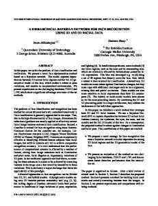
The Bayesian Network Model is an acyclic graph that encodes the conditional independence relationship of the graph nodes. There are three kinds of connections in the Bayesian Network [24] as shown in Figure 3.1. The following section discusses how the notion of conditional independence is encoded into these three types of connections.

13


3.3.1

Conditional Independence

A

B

C

(A) Serial / Causal Chain

B A

A C

C B

(B) Diverging / Common Cause

(C) Converging / Common Effect

Figure 3.1: Bayesian Network Connections

3.3.1.1

Casual Chain

For Bayesian Network Connection (A) in Figure 3.1, it translates that it is believed that A causes B to occur which further causes C to occur. If we know however that B occurred then whether A occurs or not does not affect our belief about C occurring. A is therefore conditionally independent of C given that B occurs, i.e. P (C | A ∩ B) = P (C | B). This conditional independence can also be written as (A ⊥ ⊥ C | B). 3.3.1.2

Common Cause

For Bayesian Network Connection (B) in Figure 3.1, the occurrence of B (the parent node) causes both A and C (the child nodes) to occur. If A is observed to have occurred then our belief that the occurrence of A is a result of B occurring will increase. Since our belief that B has occurred increased, it will also affect our belief that C will also occur. Therefore the occurrence of A indirectly impacts our belief that C will occur as a result of increasing the belief that B has occurred. However, if B is known to have occurred then this knowledge directly impacts our belief of C occurring regardless of whether A is observed or not. A is therefore conditionally independent of C given that B occurs, i.e. P (C | A ∩ B) = P (C | B) ≡ (A ⊥ ⊥ C | B). 3.3.1.3

Common Effect

For Bayesian Network Connection (C) in Figure 3.1, both the parent nodes A and C can cause the child node B (the effect) to occur. A and C are however

14


marginally independent (A ⊥ ⊥ C) as long as B is not known. That is to say that the probability of A occurring does not affect the probability of C occurring and vice versa, if B is not known. Therefore if A is known to occur, it will update our belief about B occurring, however it does not impact our belief about C occurring and likewise if C is known, it will not impact our belief about A occurring. However, if B is known then A and C becomes conditionally dependent, i.e. (A ⊥ 6 ⊥ C | B), which is directly opposite to the conditional independence relationship previously explained with Casual Chain and Common Cause connections. That is, if B is known to have occurred then if the probability of A increases then our belief that B was caused as a result of C occurring will decrease and vice versa. This can be expressed as P (C | A ∩ B) 6=P(C | B) ≡(A ⊥ 6 ⊥ C | B).

3.3.2

Translating Bayesian Network Model to Equations

In order to understand the methods for calculating statistical inference within a Bayesian Network Model (BNM), the first step is to be able to generate the joint probability equation based on the designed model. The following sections show how to intuitively determine the equation of a Bayesian Network Model and also illustrate how conditional independence is naturally translated from the models design. The general rule that is followed for translating a node, say X, into the Bayesian Network joint probability equation is P (X | P arents(X)) [25]. Definition 1. Joint Probability: Given two random events x ∈ X and y ∈ Y , the Joint Probability is the intersection of the events, i.e P (X = x ∩ Y = y)

3.3.2.1

BNM #1: Single Node

A Equation for BNM 1: P (A) Since there is only one node with no parents the equation of the graph is simply P (A).

15


3.3.2.2

A

BNM #2: Two Node Serial Connection

B

Joint Probability Equation for BNM 2: P (A ∩ B) = P (A) P (B | A) Breaking down the formation of the equation into steps, the first node A with no parents is simply written as P (A) while the second child node B with the parent node A is written as P (B | A). As you may have noticed, this is the same equation for conditional probability’s multiplication rule of dependent events[refer to rule definition]. Therefore since the simplest connection in the graph can be expressed in terms of a conditional probability equation, it intuitively highlights that Bayes Theorem can be applied to perform statistical inference within a Bayesian Network. 3.3.2.3

A

BNM #3: Three Nodes Serial Connection

B

C

Joint Probability Equation for BNM 3: P (A ∩ B ∩ C) = P (A) P (B | A) P (C | A ∩ B) = P (A) P (B | A) P (C | B) The first line of the equation for the BNM 3 serial connection is the same as the chain rule in conditional probability. This incorporation of conditional probability’s chain rule intuitively shows how data can be logically propagated throughout the Bayesian Network when performing statistical inference later discussed in Section 3.4. The second line is the final reduced form of the equation after considering the conditional independence relationship between A and C (see Section 3.3.1.1). That is, the probability of the node C, which a child of B and a grandchild of A, initially represented as (C | A ∩ B) is the same as P (C | B). Therefore the general rule of translating a node X to Bayesian Network joint probability equation form, i.e. P (X | P arents(X)), holds. Definition 2. Conditional Probability’s Chain Rule: For a set of n events, the chain rule states that , P (A1 ∩ A2 ∩ A3 ∩ .... ∩ An ) = P (A1 ) P (A2 | A1 ) P (A3 | A2 ∩ A1 ) .... P (An | An−1 ∩ An−2 ∩ ... ∩ A1 ).

16


3.3.2.4

BNM #4: Diverging Connection

B A

C

Equation for BNM 4:

P (A ∩ B ∩ C) = P (A) P (A | B ∩ C) P (C | A ∩ B) = P (A) P (A | B) P (C | B) Similar to as explained in BNM 3, the notion of conditional independence in Bayesian Network diverging connections results in P (A | B ∩ C) = P (A | B) and P (C | A ∩ B) = P (C | B) shown in the final line of the equation for BNM 4. This final form of the equation additionally supports that the general rule of P (X | P arents(X)) can be also directly applied to diverging connections of a Bayesian Network. 3.3.2.5

BNM #5: Converging Connection

A

C B

Equation for BNM 5: P (A ∩ B ∩ C) = P (A) P (C) P (B | A ∩ C) In this case, we note that the probability of the node B is conditionally dependent on A and C, i.e. P (B | A ∩ C) 6=P(B | C) and similarly P (B | A ∩ C) 6=P(B | A), as explained in Section 3.3.1.3. Therefore, since B has two parents, applying the general rule of P (X | P arents(X)) is shown to correctly interpret this conditionally dependency portion of the equation i.e, P (B | A ∩ C).

17

3.4 Bayesian Inference

3.4

Bayesian Inference

Bayesian Inference refers to performing statistical inference through the use of Bayes Theorem. Statistical inference is a process where conclusions are derived from probabilistic data. Therefore, statistical inference provides support for logical decision making in areas where there is uncertainty. As mentioned previously, the Digital Forensics form of Bayes’ Theorem given by Equation 3.2 is used to perform Bayesian Inference within this project as restated below:

P (H | E) =

P (E | H) P (H) P (E)

Where Hrepresents our hypothesis about an event occurring and E is the new evidence found that supports the occurrence of the hypothesis. Therefore, Bayesian Inference in the designed Bayesian Network model involves updating our belief about a hypothesis occurring based on newly observed evidence. This is essentially done by solving for the Posterior Probability P (H | E) of the main hypothesis node within the Bayesian Network. The reasoning is that the Posterior Probability P (H | E) is the conclusion / consequent of the two antecedents, the Likelihood P (E | H) and the Prior Probability P (H). The following sections discuss two methods used in the calculation of Bayesian Inference.

3.4.1

Calculation Methods of Bayesian Inference

Bayesian Inference is generally the most expensive calculation that is performed within a Bayesian Network. The two methods that are discussed in this section are (1) Inference by Enumeration and (2) Inference by Variable Elimination. However before we discuss these methods, an introduction will first be made to an expanded version of the Bayes Theorem. According Pn to the law of total probability, the Marginal Likelihood P (E) is equal to j=1 P (E | Hj ) P (Hj ). Thus, Bayes Theorem can also be written as: P (E | Hi ) P (Hi ) P (Hi | E) = Pn j=1 P (E | Hj ) P (Hj )

(3.7)

Definition 3. Law of Total Probability: For a collection of n events in the partition of a sample space S, such that it is collectively exhaustive (i.e A1 ∪ A2 ∪ A3 ∪, ..., ∪An = S) and Ai is mutually exclusive (i.e. Ai ∩Aj = for i), an event B found within the sample space S is P (B) = P (B∩A1 )+P (B∩A2 )+....+P P (B∩An ) = P (B | A1 )P (A1 ) + P (B | A2 )P (A2 ) + .... + P (B | An )P (An ) = ni=1 P (B | Aj ) P (Aj ).

18


This expanded equation is utilised in the Bayesian Inference calculation example later illustrated in Section 3.4.2. For simplification of the discussion of the following inference methods, the focus is placed on the fact that the Posterior Probability is directly proportional to the numerator product of the Likelihood and Prior Probability. That is: P (H | E) ∝ P (E | H) P (H) The Marginal Likelihood or Normalising Constant P (E) is ignored from the discussion, since it is generally a constant value and the statistical inference output value is mainly viewed by the changes in the Likelihood and Prior Probability. 3.4.1.1

Bayesian Inference by Enumeration

This is the brute force method for calculating Bayesian Inference. It involves finding the summation of all the probability values of the relevant nodes. Figure 3.2 is a diagram of the Bayesian Network that will be used to demonstrate the enumeration method for calculating Bayesian Inference.

A C

D

B Figure 3.2: Bayesian Network Inference Diagram

The Joint Probability Equation for Figure 3.2 is: P (A ∩ B ∩ C ∩ D) = P (A) P (B) P (C | A ∩ B) P (D | C)

(3.8)

For this illustration, the state of the event nodes within the Bayesian Network Figure 3.2 is either True (T ) or False (F ), i.e (A, B, C, D) ∈{T, F }. Let us say that we want to perform statistical inference to find the probability that the node A is true given that the node D is observed to be true, i.e P (A = T | D = T ). The following is the steps to derive the Bayesian Inference Enumeration method equation to calculate the answer: Step 1:

19


State the conclusion to be statistically inferred based on the formula for Conditional Probability. As previously stated in Section 3.2.2, the formulae for Bayes’ Theorem is derived from the definition of Conditional Probability. Two points to note; (1) the joint probability numerator portion of the equation only refer to the relevant nodes along the path from A to D. The node B is therefore indirectly included since C is also dependent on B. (2) The summation of all the relevant nodes is to be included except for A and D which are known to be true (T ). P P B

P (A = T | D = T ) =

C

P (A ∩ B ∩ C ∩ D) P (D)

Step 2: As aforementioned, for simplicity we will focus on the numerator portion of the equation P (A = T | D = T ) ∝

XX B

P (A ∩ B ∩ C ∩ D)

C

Step 3: Replace the joint probability equation P (A ∩ B ∩ C ∩ D) with the equivalent Equation (3.8) of the Bayesian Network.

P (A = T | D = T ) ∝

XX B

P (A = T ) P (B) P (C | A = T ∩ B) P (D = T | C)

C

Step 4: Simplify the summation by grouping event variables. This step will depend on the given equation. The aim of this step is to rearrange the equation in order to perform the least amount of calculations.

P (A = T | D = T ) ∝ P (A = T )

X

P (D = T | C)

C

3.4.1.2

X

P (B)P (C | A = T ∩ B)

B

Bayesian Inference by Variable Elimination

The Bayesian Inference by Variable Elimination goes a step further in trying to reduce the number of calculations compared to the Enumeration method. This is done by converting parts of the Bayesian Network Inference equation into pre-calculated functions. As previously stated, Bayesian Inference is the most resource intensive step to perform in a Bayesian Network. Therefore saving precalculated portions of the inference equation helps to improve the performance

20


of the Bayesian Network. The following steps illustrate the Bayesian Inference by Variable Elimination method to solve for P (A = T | D = T ) in the Bayesian Network Figure 3.2. Step 1: Perform the same steps 1 to 3 mentioned in Section 3.4.1.1 to arrive at the equation:

P (A = T | D = T ) ∝

XX B

P (A = T ) P (B) P (C | A = T ∩ B) P (D = T | C)

C

Step 2: The next step involves creating functions based on common groups of input events. The boxed portion of the equation below has the common event B. Since we already know that the event A = T it can be considered as a constant. Therefore a new function fB takes as an input parameter all possible states of C. P That is, fB (C) = B P (B) P (C | A = T ∩ B).

P (A = T | D = T ) ∝

XX B

∝

X

P (A = T ) P (B) P (C | A = T ∩ B) P (D = T | C)

C

P (A = T ) P (D = T | C) fB (C)

C

∝ P (A = T )

X

P (D = T | C) fB (C)

C

Therefore in this example the Bayesian Inference by Variable Elimination Method reduced the need to calculate for event B by incorporating the precalculated figures in a function named fB (C).

3.4.2

Bayesian Network Example

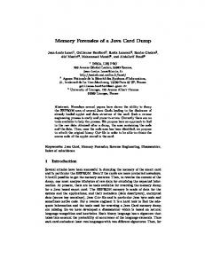
In this section we will illustrate how Bayesian Inference is performed using the Enumeration method. In essence this example will incorporate all the concepts mentioned in this Chapter. Figure 3.3 is a diagram of the Bayesian Network that will be examined. This Bayesian Network has been set up with the Netica [26] software.

21


Figure 3.3: Bayesian Network Example

This is the general structure of the Bayesian Network that is used in the development of MemTri. The top-most nodes prefixed with H are referred to as hypothesis nodes while the lowest level nodes prefixed with E are referred to as the evidence nodes. To make this example more intuitive the nodes have been assigned specific meanings as follows: H: The suspect employee’s computer was used to send confidential company files to a third party using FTP H1: An FTP connection was established between employee machine and third party E1: Network Logs show a TCP connection on port 21 between employee machine and third party E2: FTP ”Transfer OK” response packet found between employee machine and third party in router cache The probability values shown in Figure 3.3 is the Prior Probability values of the Bayesian Network. The following joint probability tables 3.1, 3.2 and

22


3.3, represent the Likelihood probability values that is associated with the given Bayesian Network in Figure 3.3:

H1 H

Yes

No

Uncertain

Yes

60

35

5

No

35

60

5

Uncertain

5

5

90

Table 3.1: Likelihood Joint Probability Table for P(H1 | H)

E1 H1

Yes

No

Uncertain

Yes

85

15

0

No

15

85

0

Uncertain

0

0

100

Table 3.2: Likelihood Joint Probability Table for P(E1 | H1)

These probability values are usually set based on the data gathered from experts in the field of the investigation. From the table we see that a node has three states ‘Yes’, ‘No’ or ‘Uncertain’. An important point to note is that the probabilities in the Bayesian Network must add up to 100%. Now let us say that an investigator wants to determine the probability that the suspect employee sent confidential files to a third party given that he has observed that there was a FTP ‘Transfer OK’ packet found. In other words, the investigator wants to determine P (H = Y | E2 = Y ). This hypothesis can be examined by performing Bayesian Inference. Statistically inferring a conclusion for this hypothesis can be useful in aiding the investigator to confidently decide whether the investigation is worth a certain dedication of resources. Now the nodes encountered from H to E2 are (H, H1 and E2). There are also no additional parent nodes that has to be considered. Therefore the joint

23


E2 H1

Yes

No

Uncertain

Yes

75

25

0

No

25

75

0

Uncertain

0

0

100

Table 3.3: Likelihood Joint Probability Table for P(E2 | H1)

probability equation for the portion of the Bayesian Network needed for inference is: P (H ∩ H1 ∩ E2) = P (H) P (H1 | H) P (E2 | H1) Applying the Enumeration method for calculating Bayesian Inference, the equation that is needed to evaluate the investigator’s request is: P P (H = Y | E2 = Y ) = = =

∩ H1 ∩ E2) P (E2) P P (H = Y ) P (H1 | H = Y ) P (E2 = Y | H1)) H1 P (E2 = Y ) P P (H = Y ) H1 P (H1 | H = Y ) P (E2 = Y | H1)) P P H H1 P (H) P (H1 | H) P (E2 = Y | H1)) H1 P (H

Solution: .333 [(.6 × .75) + (.35 × .25) + (0.05 × 0)] .333 [.45 + .0875 + 0] .333 = .333 = 0.5375

P (H = Y | E2 = Y ) =

≈ 0.538 Therefore the probability that the employee sent the files to a third party given the FTP packet evidence found based on Bayesian Inference is 0.538. This can be seen visually in Figure 3.4.

24


Figure 3.4: Bayesian Network with Observed Evidence Example

25

Chapter 4

Volatile Memory This chapter presents some fundamental concepts of how volatile memory is utilised within a Personal Computer (PC). The discussion focuses primarily on main memory or Dynamic Random Access Memory (DRAM), which is the type of memory captured and analysed in this project. It is important that a Digital Investigator understands how data is stored in main memory, in order to verify the completeness of a collected memory image and to ensure accurate analysis of its contents. Additionally, it improves the Digital Investigator’s ability to debug possible output result errors from memory analysis tools such as Volatility [6] and to assess how malware may attempt to hide itself from being discovered by such tools. This chapter also explains some of the important considerations that a Digital Forensics Investigator should take into account when deciding what tool to use to collect the main memory contents of a computer. The improper choice of tool and methodology can result in an incomplete/inaccurate memory capture image.

4.1

Computer Memory

Memory within a computer are physical devices that store information. There are two types of memory within a computer system, non-volatile memory and volatile memory. Non-volatile memory, also referred to as permanent storage, does not lose the information it stores when the device is powered off. Two examples of non-volatile memory devices are magnetic hard disks and Erasable Programmable Read-Only Memory (EPROM). Volatile Memory on the other hand stores information temporarily, in that, the information it stores is lost when the device is powered off. Two examples of volatile memory devices are DRAM and the Central Processing Unit (CPU) registers. Though volatile RAM devices and hard disks are both computer memory, it is common to refer to volatile RAM devices as ‘memory’ or ‘primary memory’ and hard disks as ‘secondary storage’. The main focus of this project is the analysis of DRAM or main memory. From this point the word ‘memory’, if used alone, will refer to the computer’s main

26

4.2 PC Architecture

memory and likewise the acronym RAM will refer to DRAM.

4.2

PC Architecture

Understanding the layout of a PC’s Architecture can help to better comprehend how memory is accessed within a computer and therefore how to develop tools to capture the contents of memory. It also informs the Investigator of the various considerations that must be taken into account in order to obtain a memory image that is both correct and complete. The following sub-sections briefly explain two main components of a modern PC’s architecture (see Figure 4.1) in relation to memory forensics. The first component, which is the Memory Management Unit (MMU), is mainly utilised for software based memory acquisition (see Section 4.6.2), while the second Direct Memory Access Controller (DMA) component is mainly utilised for hardware based memory acquisition (see Section 4.6.1).

Figure 4.1: Physical Layout of a modern computer system [1]

4.2.1

Memory Management Unit

The Memory Management Unit (MMU) is a part of the CPU and is mainly responsible for translating an address requested by the processor into the actual

27

4.3 CPU Architecture

physical memory address in RAM. In order to speed up the address translation process, the MMU communicates with the Translation Look-aside Buffer (TLB) which is a fast access temporary storage for address translation structures. The implementation of the address translation process (see Section 4.4.2.1) however varies based on the type of CPU architecture.

4.2.2

Direct Memory Access (DMA) Controller

The Direct Memory Access (DMA) Controller allows I/O devices to access main memory directly without the need to contact the CPU. This therefore improves the performance of the entire system by freeing up the CPU to focus on the processing of other tasks. Since the DMA facilitates direct access to main memory for I/O devices, it has been utilised by Digital Forensics Investigators as a means for acquiring a memory image from a target computer (see Section 4.6.1).

4.3

CPU Architecture

The mechanism by which a computer’s memory address space is accessed is dependent on the architecture of the Central Processing Unit (CPU). This project utilised Intel’s IA-32 architecture. IA-32 is the 32-bit family of Intel’s microprocessor architecture and is also referred to as x86 or i386. Intel’s IA-32 architecture supports up to 4GB of memory however this can be expanded to 64GB using the Physical Address Extension(PAE) paging feature. Intel’s IA-32 architecture has three modes of operations namely protected mode, real-address mode and system management mode [2]. Throughout the remainder of this chapter, the discussion will be in reference to Intel’s IA-32 microprocessor running in protected mode, which supports features such as segmentation, paging and virtual memory. Before explaining each of these features however, Sections 4.3.1 and 4.3.2 will define two sets of volatile memory devices located within the CPU, namely registers and caches respectively. Additionally, a few of the specialised registers and caches relevant to memory management will be briefly introduced.

4.3.1

Registers

Registers are devices with a small amount of memory that can be accessed quickly by the CPU. The group of registers involved in the basic execution of a program are the general purpose registers, segment registers, EFLAGS register and EIP register [2]. There are eight general purpose registers which are responsible for storing operands and pointers. The EFLAGS register stores the status of a program’s execution and allow application level control of the CPU. The EIP register stores a pointer to the next instruction to be executed. The segment registers store up to six segment selectors which are pointers used to locate segments in memory. The three main segment selectors are named after the segmented parts of the program being pointed to, i.e. CS (Code Segment), DS (Data Segment)

28

4.3 CPU Architecture

and SS (Stack Segment). The other three segment selectors point to data segments of a program and are namely ES, FS and GS. Section 4.4.1 will explain how the segment selectors, stored within the segment registers, play a role in segmentation memory management. The IA-32 microprocessor additionally has four registers responsible for locating data structures that control segmented memory management, namely GDTR (Global Descriptor Table Register), LDTR (Local Descriptor Table Register), IDTR (Interrupt Descriptor Table Register) and TR (Task Register). Collectively these registers generally contain linear base addresses, segment limits, table limits and segment selectors. Another set of registers involved in memory management are the control registers. There are five control registers label CR0, CR1, CR2, CR3 and CR4. The way in which these control registers are involved in memory management are, (1) through the use of flag bits that set and control the paging mode of operation and (2) by defining the base address to the first paging structure. Further details about how specific control registers control the paging memory management system is explained in Section 4.4.2. Note that each core within the CPU generally has their own set of the registers that were mentioned throughout this section.

4.3.2

Cache

A cache is a high speed device, normally implemented using Static RAM (SRAM), that temporarily stores small copies of main memory, in order to speed up the average time it takes to access main memory data. The CPU generally contains a hierarchy of data and instruction caches that are referenced by levels (L1, L2, L3 .. etc). The lower the cache level the faster it is to access but the smaller the storage size. Conversely, the higher the cache level the slower it is to access and the larger the storage size. In order to speed up the translation of a virtual address to a physical address, a specialised cache named the Translation Look-aside Buffer (TLB) was implemented as part of the MMU in the CPU (see Figure 4.1). A virtual address is explained in further detail in Section 4.4.2 and is simply a linear address that is produced when paging mode is turned on. The TLB stores the physical address that corresponds to the page number portion of a virtual address. Therefore, the CPU first quickly checks for a matching entry in the TLB, before attempting to perform the entire page translation process using main memory. The TLB also contains information about the access rights to a page and a dirty flag that indicates if the page has been modified since it has been placed in the TLB. Another cache used to speed up the page translation address process is the Page Directory Entry (PDE) cache. This cache stores PDEs that is used to locate the page table. Therefore with the PDE cache, the CPU still has to complete the address translation process by locating the page table and ultimately the physical address; however it is still quicker than having to access the PDE from

29

4.4 Memory Management

main memory.

4.4

Memory Management

This section discusses two memory management mechanisms namely segmentation and paging. An overview of these memory management mechanisms can be seen in Figure 4.2. Memory management techniques are designed to allow the computer system to utilise its available memory efficiently, to prevent corruption of multiple programs during execution and to avoid scenarios that can cause a program to crash. The addressable memory space of the IA-32 microprocessor is referred to as the linear address space [2]. The CPU’s linear address space allows a running program to view memory as a single continuous byte addressable space with an address range from 0 to 232 −1. An address for any byte within the linear address space is referred to as an linear address [2]. The MMU is responsible for translating various forms of memory addresses to the actual physical address in memory.

Figure 4.2: Segmentation and Paging Process [2]

30


4.4.1

Segmentation

When the IA-32 microprocessor is running in protected mode, segmentation is always enabled. Segmentation involves dividing the processor’s linear address space into variable length address spaces referred to as segments [2]. As hinted by the types of segment registers in Section 4.3.1, segments point to code, data and stack portions of a program’s execution in memory. In this way segmentation allows for multiple programs to run on the same processor without execution collisions, through the isolation of each program’s code, data and stack information. The address used to locate a byte within a segment is referred to as a logical address [2]. The logical address consists of a 16 bit segment selector and an 32 bit offset. The segment selector is a unique identifier for a segment and points to record in the Global Descriptor Table (GDT) or Local Descriptor Table (LDT). The corresponding segment selector record in the GDT or LDT contains the base address of the segment within the linear address space. The base address of the segment is then added to the offset portion of the logical address to produce the linear address of the requested byte within the segment. The recently explained translation process of a logical address to a linear address is summarised in Figure 4.3. If paging is disabled then the CPU’s linear address is the same as the memory’s physical address. A physical address refers to the actual address in main memory where the data is located. If paging is enabled then a page address translation process has to be done to convert the linear address to a physical address, which is later explained in Section 4.4.2.1.

Figure 4.3: Translation of Logical Address to Linear Address [2]

4.4.2

Paging

Paging is enabled by setting the PG flag (bit 31) in the CR0 register to 1. The paging mechanism in IA-32 architecture, divides the linear address space into fixed address space sizes referred to as page frames. Paging is used to implement

31


virtual memory through a mechanism called demand paging [1]. With demand paging, a file on secondary storage device can be used to store page frames from main memory. Page frames can then be swapped into and out of main memory when needed using the page file, through a process referred to as swapping. Therefore, demand paging allows for the execution of multiple programs which collectively require more memory space than is available in main memory. However, it is an expensive operation to access a page frame that is stored within a page file. Also if the computer system spends a considerable amount of time fetching page frames from the page file, it can significantly degrade the performance of the system. This is referred to as thrashing [1]. There are three paging modes namely 32-bit paging, PAE paging and IA-32e paging. These modes are mainly set by flags within the CR0 and CR4 control registers. PAE paging mode allows for 32-bit linear addresses to point to a 64-bit physical addresses and supports a maximum of 64GB of memory. IA-32e paging mode is used only by processors that support Intel 64 architecture and allows for 48-bit linear addresses that support up to 512GB of memory. The main focus of the discussion however will be on the 32-bit paging mode which uses a 32-bit linear address space and supports a maximum memory size of 4GB. When paging is turned on, a linear address is also referred to as a virtual address. A virtual address has two parts, a page number at the higher bit portion and an page frame offset at the lower bit portion of the address. Note that the IA-32 architecture is a little-endian based architecture. The number of bits of the virtual address assigned to the page number and the page frame offset depends on the page frame size. If the page frame size used is 4MB, the higher 10 bits of the virtual address is the page number and the lower 22 bits is the page frame offset as illustrated in Figure 4.4. In this case the page number represents the offset in the Page Directory structure where the page frame’s base address is stored. 31

|

22 21

Directory {z

page number

0

Offset }

Figure 4.4: Virtual Memory Address for 4MB page size

However, if the page frame size is 4KB, the higher 20 bits of the virtual address is the page number while the lower 12 bits is the page frame offset as illustrated in Figure 4.5. In this case the higher 10 bits of the page number represents the Page Directory offset while the lower 10 bits of the page number is the Page Table offset (see Figure 4.5). The following section 4.4.2.1 will explain how a virtual address is translated to a physical address when 4KB pages are used. All variations of the paging mode settings uses a similar concept for locating the paging structures needed to perform page address translation as discussed in Section 4.4.2.1.

32

4.4 Memory Management 31

22 21

Directory |

12 11

Table {z

0

Offset }

page number

Figure 4.5: Virtual Memory Address for 4KB page size

4.4.2.1

Page Address Translation

Figure 4.6: Translation of Virtual Address to Physical Address for 4KB page size [2]

The conversion of a virtual address (VA) to a physical address starts with the CR3 register. The bits 31:12 of the CR3 register contains the base address for the Page Directory structure (see Appendix A). After locating the Page Directory, the Page Directory offset bits 31:22 of the VA (see Figure 4.5) is used to select the relevant Page Directory Entry (PDE). Each PDE in the Page Directory is 4bytes (32 bits) therefore the Page Directory offset has to be multiplied by 4 and added to the Page Directory base address in order to locate the PDE. Figure 4.7 shows the combination of the Page Directory’s base address in the CR3 register and the Page Directory offset in the VA, which together forms the PDE address. Note that the two lowest bits with value 0 represent a shifting of the Page Directory offset two bits to the left, which essentially multiplies the offset by 4. CR3[32 : 12] |

VA[32 : 22] {z

PDE Address

00 }

Figure 4.7: Combination of base address in CR3 register with Directory offset in VA to produce the PDE Address

33

4.5 Windows Operating System Process

The next step in the page translation process involves locating the Page Table Entry (PTE) for the PDE.The PDE contains the base address of the Page Table in bits 31:22 (see Appendix A). After locating the Page Table, the offset in the VA bits 21:12 is used to select the relevant PTE. The PTE is 4 bytes in size therefore the Page Table offset has to be multiplied by 4 in order to locate the PTE. Figure 4.8 shows the combination of the Page Table’s base address in the PDE and the Page Table offset in the VA, which together forms the PTE address. PDE[32 : 12] |

VA[21 : 12] {z

PTE Address

00 }

Figure 4.8: Combination of base address in PDE with Page Table offset in VA to produce the PTE Address

The final step in the page translation process involves locating the physical address requested within the page frame using the PTE. The bits 31:12 of the PTE contains the base address of the page frame (see Appendix A). After locating the page frame, the page frame offset in bits 11:0 of the VA is used to locate the physical address requested in main memory. Figure 4.9 shows the combination of the page frame’s base address in the PTE and the page frame offset in the VA, which together forms the actual physical address in main memory requested by the CPU. PTE[32 : 12] |

VA[11 : 0] {z

Physical Address

}

Figure 4.9: Combination of base address in PTE and with Page Frame offset in VA to produce the Physical Address

The entire page translation process can be seen in Figure 4.6. Note that there are bits within the CR3 register, PDE and PTE that contain page control information. For example bit 6 (dirty flag bit) of the PTE is used to indicate whether the page has been updated by another application and thus needs to be refreshed in memory and the page file (see Appendix A).

4.5

Windows Operating System Process

This section gives information about the structure of a Windows operating system (OS) process and highlights some of the key fields that are particularly interesting in memory forensics investigations. This section also discusses the different techniques that are used to locate processes within a Windows OS memory image and explains how malicious users may attempt to hide a process. Therefore, by understanding the structure of a Windows OS process, a digital forensics investigator can fine tune his search for evidence and also detect attempts to hide

34


data. However, before going into details about the structure of the Windows OS process, a brief description is given of the Windows OS’s architecture.

4.5.1

Windows OS Architecture

The Windows OS was developed by Microsoft and has two modes in which a program can be executed, i.e. user mode or kernel mode (see Appendix B). Applications ran by a user is generally executed in user mode. In user mode an application has restricted access to system resources. Therefore, a user mode application generally cannot directly access/update the contents in the physical DRAM (main memory) and must first make a request via kernel mode functions which has unrestricted access to system resources. This communication between user mode and kernel mode is facilitated through the Executive (System) Services which is a part of the Windows Executive component of the OS (see Appendix B). As defined by Microsoft, “the Executive is a family of software components that provide the basic operating system services” [27]. In the Windows OS, resources are represented using data structures referred to as ‘objects’. These objects are generated, managed and protected by the Object Manager which is a part of the Windows OS Executive. Appendix C shows a list of some of the objects managed by the Object Manager. The EPROCESS object (see Appendix C) is what is used to represent and manage the execution of a process in the Windows OS environment. More details are given about the EPROCESS structure in Section 4.5.2. An important module within Windows’ kernel mode is the (micro)kernel itself (see Appendix B). The kernel is comprised of the core components for the functioning of the OS. The kernel also acts as an interface between the Executive and Hardware Abstraction Layer (HAL) to enable key OS features such as threading, context switching and multiprocess synchronisation.

4.5.2

Windows Process Structure and Resources

This section takes a closer look at the EPROCESS object structure (see Table 4.1) that is used to implement a Windows Process. When the Windows OS generates a new process, it builds various data structures that are used to manage the process’ resources. The EPROCESS object usually contains pointers to these resource management data structures instead of storing them inside the EPROCESS object itself. Figure 4.10 shows the five main resources managed by a Windows Process namely threads, virtual address space, handles, security access and loaded modules. The fields in the EPROCESS object structure (see Table 4.1) that are used to manage these five resources will be briefly discussed in the following subsections.

35


Figure 4.10: Basic Resources of a Process [1]

4.5.2.1

Windows Process Object

Before discussing the major data structures used to manage the resources of a Windows process, this section takes the time to introduce a few data fields that describe information about the process itself. These field therefore can provide key forensic information about the state of the process at the time the memory image was captured. The first field in the EPROCESS object (see Table 4.1), pcb, is the kernel’s process control block which manges the state of the process and stores the process’ crucial register values during context switching. One of these key register value fields within the pcb structure is the DirectoryTableBase (DTB), which is loaded into the CR3 register in order to perform page address translation (see Section 4.4.2.1). Volatility’s [6] ‘memmap’ plug-in therefore uses this pcb.DirectoryTableBase field when performing calculations to map a process’ virtual address space to its physical address space. The CreateTime and ExitTime fields (see Table 4.1) store the time the process was executed and terminated respectively. It is important to note that when a process exits, its allotted virtual address space is simply marked as free similar to what is done by most file systems when a file is deleted [13]. The length of time the process structure remains in memory before being overwritten depends on the amount of system activity.

36


>>> dt(” EPROCESS”) ’ EPROCESS’ (704 bytes) 0x0 : Pcb 0x98 : ProcessLock 0xa0 : CreateTime 0xa8 : ExitTime 0xb0 : RundownProtect 0xb4 : UniqueProcessId 0xb8 : ActiveProcessLinks 0xc0 : ProcessQuotaUsage [snip] 0xf4 : ObjectTable 0xf8 : Token [snip] 0x140 : InheritedFromUniqueProcessId [snip] 0x16c : ImageFileName [snip] 0x188 : ThreadListHead [snip] 0x198 : ActiveThreads [snip] 0x1a8 : Peb [snip] 0x278 : VadRoot

[’ KPROCESS’] [’ EX PUSH LOCK’] [’WinTimeStamp’, ’is utc’: True] [’WinTimeStamp’, ’is utc’: True] [’ EX RUNDOWN REF’] [’unsigned int’] [’ LIST ENTRY’] [’array’, 2, [’unsigned long’]] [’pointer’, [’ HANDLE TABLE’]] [’ EX FAST REF’] [’unsigned int’] [’String’, ’length’: 16] [’ LIST ENTRY’] [’unsigned long’] [’pointer’, [’ PEB’]] [’ MM AVL TABLE’]

Table 4.1: Volatility’s volshell command output for the EPROCESS structure

The UniqueProcessId field stores a positive integer that uniquely identifies a process and is usually referred to as the “PID”. The parent process’ PID that spawned a (child) process, is stored in the InheritedFromUniqueProcessId field. In Windows however, the parent child relationship between processes is different than in Linux. In Linux, if a parent process closes then the child process(es) terminates as well. With Windows however, if a parent process terminates, the child process still continues to run. The InheritedFromUniqueProcessId is also not updated after being initially set. The ImageFileName field stores up to 16 ASCII characters for the process’ executable filename. Longer unicode versions of the filename can be found in a VAD node or in the Process Environment Block (PEB). 4.5.2.2

Handles

A handle is simply a pointer to an opened instance of resource object that is managed by the kernel [1]. A resource object, as listed in Appendix C, can be

37


a file, thread, mutant or registry key etc. The EPROCESS.ObjectTable points to a HANDLE TABLE which uses a TableCode to identify where the list of table entries are stored (see Figure 4.11). The handle table can store up to 512 handle entries for a 32-bit system and 256 for a 64-bit system. Each handle entry in turn contains an Object field that points to the actual OBJECT HEADER(s) of the object(s) being referenced by the EPROCESS structure. Therefore, by enumerating the handle entries opened by a Windows process, a Digital Investigator can gather valuable information about the kernel resources that the process had access to, which in-turn can help paint a story of what the process was doing on the system.

Figure 4.11: Diagram showing how an Object is referenced in the Object table of a Process [1]

4.5.2.3

Tokens: Security Access

Before a process can access a resource, the kernel must assess whether it has the adequate permission(s) to do so. In Windows, a token ( EPROCESS.Token) is used to define the security context of a process. The token stores information about the security identifiers (SIDs)/user accounts associated with the process and the privileged tasks that can be performed. Therefore, analysing tokens can give the Digital Investigator valuable information about whether an attacker may have been able to compromise a process and increase its level of access to have an Administrative (account) access. Similarly, an attacker may have also performed a ‘privilege escalation attack’ on a process to allow it to perform a task that would otherwise be restricted. 4.5.2.4

Threads

A process itself does not perform the work of an application but rather schedules basic tasks which are executed via threads. When a process is generated, it has

38


at least one thread which is referred to as the ‘primary thread’. A process can generate and execute multiple threads which share the process’ resources such as the code segments, global variables, opened files and the process environment block (PEB) as illustrated in Figure 4.12. A thread however has its own stack and a Thread Local Storage (TLB) pointer which is used to store data unique to each thread [28] (see Figure 4.12).

Figure 4.12: Diagram showing shared and independent resources of Process and Threads [3]

Windows uses a doubly linked list to manage the list of threads for a process and the head node is saved in the field EPROCESS.ThreadListHead (see Table 4.1). Later in Section 4.5.3, it discusses how to enumerate through doubly linked list structures, which can reveal key insights about the various (thread) tasks being performed by the process at the time the memory image was captured.The EPROCESS also maintains the number of ActiveThreads (see Table 4.1), which if 0, is an indication that the process has terminated. 4.5.2.5

Virtual Address Descriptors

Each windows process references its own private virtual memory/address space that is isolated from other processes via the segmentation memory management feature [29]. A portion of a process’ virtual address space is allocated as user(-

39


mode) space and the remaining as kernel(-mode) space. The boundary between user and kernel space is defined by the MmHighestUserAddress field located within the Kernel Debugger ( KDDEBUGGER DATA64) structure. As shown in Figure 4.13, the resources of a process such as the thread stack, process heap, PEB and DLLs are generally stored in the user space of the process. In cases where the process has to access a shared kernel DLL or driver, it would first make an request for access through Windows Executive Services. If successful, the kernel DLL or driver is referenced from the kernel space region of the process’ virtual address space (see Figure 4.13).

Figure 4.13: Process’ virtual address space and stored resource areas [1]

In order to manage the virtual address space of a Windows process, a Virtual Address Descriptor (VAD) tree structure is used. The root of the VAD tree is stored in the field EPROCESS.VadRoot (see Table 4.1). Each VAD node stores the start and ending virtual address range that it represents/manages. It also stores descriptive information about the data that is contained within the allotted virtual address range; such as whether the data belongs to a memory map file, process heap or thread stack, and the access rights to that specific virtual address space such as read, write and/or copy. The VAD tree is structured as a self-balancing tree such that lower virtual memory ranges are connected to the

40


left and higher memory ranges to the right. There is also a flag (i.e. MemCommit) within the VAD tree node which specifies whether the virtual memory region has been committed to memory. The ‘memdump’ plug-in provided by Volatility [6] to dump a process’ memory to a file, therefore enumerates the entire VAD tree and dumps only the ‘committed’ virtual address ranges. Note that since the process’ VAD tree references virtual addresses, page translation has to be performed in order find the corresponding physical address in memory where the data is actually stored. Therefore, though data stored in the process’ virtual address space may appear to be continuous, in reality the data can be scattered in different parts of the physical RAM. 4.5.2.6

Process Environment Block

The Process Environment Block (PEB) structure ( EPROCESS.Peb) contains information about loaded modules such as DLLs and executable files, along with process heap and environment variable information. The PEB therefore contains a rich set of information that can prove valuable in a memory forensics investigation. For example, the full path of the process’ executable and DLLs, along with the command line that started the process, can be found in the PEB [1]. The environment variables mainly contain directory paths which are searched when a call is made to execute a file. Attackers may manipulate environment variables in order to get their maliciously prepared file to execute instead of the proper file requested by the user. The process’ heap generally store dynamic data sent to the process. This includes for example, typed input by the user into an application such as notepad, which Ligh [1] demonstrates can be skilfully retrieved by examining the VAD tree nodes that hold process heap information.

4.5.3

Enumerating Windows Processes

There are two main techniques for enumerating through the processes within a memory image, namely doubly linked list enumeration and pool scanning. The doubly linked list enumeration method, which is implemented in Volatility’s [6] ‘pslist’ plug-in, involves enumerating the doubly linked list of active process found in the field EPROCESS.ActiveProcessLinks (see Table 4.1). The head of this doubly linked list is pointed to by the PsActiveProcessHead field found within the Kernel Debugger structure ( KDDEBUGGER DATA64). Volatility’s [6] ‘kdbgscan’ plug-in is able to locate this KDDEBUGGER DATA64 structure by scanning the input memory image for a ’kdbg’ signature, similar to file carving for files on a disk image. Each doubly linked list of an active process (i.e. EPROCESS.ActiveProcessLinks) contains two pointers, namely flink and blink, which essentially points to the next and previous active process respectively. Therefore, a list of all the active processes can be generated by first locating of the head EPROCESS.ActiveProcessLinks node, which is pointed to by the field KDDEBUGGER DATA64.PsActiveProcessHead, then enumerating

41


through the list using the flink/blink pointers. This technique for locating processes is however susceptible to Direct Kernel Object Manipulation (DKOM) attacks [4]. As shown in Figure 4.14, a DKOM attack can be done to hide a process by manipulating the blink/flink pointers to effectively unlink a process from the list. In this case, Volatility’s [6] ‘pslist’ plugin will not identify the hidden/unlinked process as part of its results.

Figure 4.14: DKOM attack on EPROCESS structure to hide a process [4]

The pool scanning technique however is not susceptible to DKOM attacks. This is because the pool scanning technique, implemented in Volatility [6] as the ‘psscan’ plugin, involves searching for PoolTag values located within the POOL HEADER attached to Windows Executive Objects, and therefore is not dependent on the fields of the EPROCESS Object. The POOL HEADER essentially contains debugging information for the Object (e.g the EPROCESS Object) structure to which it is attached. It also specifies if the Object is paged (i.e. can be written to secondary storage) or nonpaged (i.e. never written to secondary storage). Note that EPROCESS Objects are always set as nonpaged. The PoolTag value for an EPROCESS Object can be either ‘Proc’ or ‘Pro3’ [1]. Therefore, to locate all the processes within a memory image using pool scanning involves searching for the aforementioned PoolTag values. However, just searching for these values alone can lead to a lot of false positive process identification results. To reduce false positives, the psscan plug-in also utilises the known structure of the fields within the POOL HEADER and Windows Executive Object structures to confirm a positive match. Therefore after locating the process’ PoolTag value, if a field at a particular offset in the POOL HEADER or EPROCESS structure is known only to have the value 0 or 1, but another value is found, it will identify the match as a false positive and not include it in the final results. Another noted advantage of the pool scanning technique is that it is able to identify processes that have been terminated and removed from the list of active processes, however have not yet been overwritten in main memory.

42

4.6 Memory Acquisition

4.6

Memory Acquisition

Due to the volatile nature of main memory and its utilisation for concurrent processing within a computer, careful planning is required to ensure that the memory image collected is both accurate and complete. Therefore, the memory collection planning phase is especially important since the court will not accept evidence that is likely to be unreliable or inaccurate. Vomel et al. [12] proposed three criteria for measuring the ‘forensic-soundness’ of a memory image which are correctness, atomicity and integrity. The correctness of a memory image has to do with whether the values at a specific location in the memory image match the actual values that were stored at that same requested location in the physical RAM device, at the time the memory snapshot was taken [12]. An example of how the correctness of an image can be impacted is through the presence of a rootkit that redirects the request to read a location in memory to another incorrect location. The atomicity is the consistency measure of the concurrent activity captured within a memory image [12]. According to Gruhn and Freiling[30], generally the smaller time span between acquiring the first and last memory regions, the better the atomicity. The integrity measures how many memory region values have changed in the memory image from the specific time the Digital Investigator started the capture via the memory acquisition tool. For example, with software based acquisition, the captured memory image’s integrity will not be perfect since portions of the memory is changed when the acquisition program is loaded. There are generally two categories of memory acquisition tools, i.e. hardware based (see Section 4.6.1) or software based (see Section 4.6.2). The following sections discuss various memory acquisition methods along with their strengths and weaknesses based on the ‘quality’ of the image produced. Since all memory acquisitions methods have strengths and weakness, the Digital Investigator must be aware of this in order to select the best method based on the resources available. Another point to note is that if paging is turned on then some of the page frames for a process can be located on disk and not in main memory. In such cases, some memory data may be absent from the memory image.

4.6.1

Hardware-based Methods

Hardware-based methods have generally been considered the most secure way to obtain an accurate memory image since it does not depend on running software on the OS that can be subverted by malware. Hardward-based acquisition methods also do not require the computer to be in a logged in state in order to execute a program as with software based acquisition methods. However, hardware-based memory acquisition is generally more costly to implement than software-based methods and the acquisition methods are limited to the hardware that is available in the target machine. The Digital Investigator also must have knowledge of various kinds of hardware and configurations since there are usually risks involved

43


that can possibly destroy or hinder the memory content from being acquired. In the following sub-sections, the strengths and weaknesses of the two main types of hardware-based acquisition methods, namely ’DMA Attack’ and ’Cold Boot Attack’, are discussed in terms of the ’forensically-soundness’ [12] of the memory image produced. 4.6.1.1

DMA Attack

A DMA Attack involves accessing the main memory of a computer directly via the DMA controller. A DMA Attack is usually performed through the use of a Peripheral Component Interconnect (PCI) device [31] or FireWire. Unlike with FireWire methods, the PCI device methods may require the device’s driver to already be installed on the target system. Therefore, in the case where the PCI device driver has to be installed, the target machine must be logged in with a user that has adequate permissions to do so. Though DMA Attack techniques do not rely on the CPU, which is typically easier to compromise by malware during memory acquisition, there are various ways the correctness of a memory image produced can be affected. For example, with PCI DMA Attack methods, the installed driver can be compromised by a malware [32] that redirects memory address requests to other parts of memory in order to hide itself from being included in the memory capture image. Rutkowska [33] also identified that kernel-level malware (i.e. rootkits) can change the values in the registers used by the DMA controller to locate a memory address and therefore can compromise the correctness of the acquired image. According to an evaluation of the different types of memory acquisition methods, Gruhn et al. [30] identified that simple straight-forward DMA Attack methods generally appear to have the worst atomicity rating. This is because the system is actively updating memory while the acquisition process is taking place. A solution to this problem on a system that uses an Intel IA-32 microprocessor is to utilise the System Management Mode (SMM) of operation. Reina et al.[34] explains that when the processor switches to SMM via a System Management Interrupt (SMI), the system enters a suspended state therefore allowing a consistent snapshot of the memory to be captured. However as previously hinted, this solution is limited to the system containing a suitably configured Intel IA-32 microprocessor. The integrity of straight-forward DMA Attack methods appear also to have the worst integrity rating [30]. This is because memory acquisition using DMA is slow [32], and so the data that exists in memory when the investigator started the acquisition process is far different from the data in the final memory image. The SMM solution with Intel IA-32 microprocessors as previously mentioned can also solve this problem. Issuing the SMI to suspend the system is almost immediate and therefore the investigator can capture the full contents of memory that were available the moment he started the acquisition process. Another factor that can degrade the integrity of the memory image captured via the PCI DMA Attack

44


method, is if the PCI device drivers has to be installed. This installation means that the driver install program has to be executed, which will overwrite contents in memory; thus the captured memory contents will definitely be different from the initial content stored right before the Investigator started the acquisition process. Another limitation that the Digital Investigator should be aware of is that FireWire and PCI devices commonly can only capture up to 4GB of memory, due to the 32-bit addressing limit of some device ports. This limitation is an issue since it is becoming more common for computer systems to have over 4GB of memory. There are 64-bit PCI cards that are able to capture more than 4GB of memory. However, if the hardware of the computer only supports 32-bit PCI slots then this will limit the maximum amount of accessible memory to 4GB. A risk that the Digital Investigator should also consider is that the attacks identified by Rutkowska [33] can cause the computer system to crash while performing DMA Attack based memory acquisition. This could further result in the Digital Investigator facing legal charges for damages to a system [33]. 4.6.1.2

Cold Boot Attack

A Cold Boot Attack is performed by powering off a computer and then extracting the contents from RAM. This technique is made possible due to the RAM remanence effect [35] which describes the phenomenon of DRAM losing bits gradually over time after being powered off. Halderman et al. [36] further showed that cooling DDR1 and DDR2 RAM chips using a simple ‘canned air’ duster spray, before powering off the computer, can slow down the rate of bit degradation. Another method of cooling can be to immerse the RAM modules in liquid nitrogen which can allow the RAM to maintain over 99% of its contents outside of a machine for over an hour [36]. There are generally two ways to perform a Cold Boot Attack. The first way involves simply rebooting the machine by briefly removing and restoring power to the computer, which is referred to as cold booting [36]. This is different from warm booting, which is initiated by performing an operating system restart, in that power is not removed from the computer during reboot. Though no bits are lost from RAM during warm-boot compared to cold-boot, there is a risk that a software can be triggered to wipe key information from RAM when the operating system restart procedure is initiated. After performing the cold-boot, the target computer’s BIOS can be configured to boot a memory imaging tool from a USB drive. The second method of performing a Cold Boot Attack involves taking the DRAM modules from the target machine and inserting them into another computer that is setup to capture the DRAM’s contents when booted [36]. Transferring the DRAM modules may mean more bit degradation since it would likely take a longer time to refresh the RAM’s power than with the first method of simply rebooting. However this method is more secure since the target machine may be set to wipe the RAM during the Power-On Self Test (POST) stage performed by the BIOS [36].

45


According to the results obtained by Gruhn et al. [30], the quality of the memory image produced by a Cold Boot Attack is superior to simple DMA Attack methods with regards to atomicity and integrity. Cold Boot Attack method is described to have perfect atomicity [30] in that, the contents of the RAM is essentially ‘frozen’ at the point in time when the power is removed from the computer and is no longer affected by system activity when the memory image is acquired. The Cold Boot method is also described to have almost perfect integrity [30] in that, at the point the Investigator decides to collect a memory image by removing power from the computer, the only change that is made to the RAM is caused by the loading of the imaging tool. The imaging tool is usually implemented with a small boot loader program such as syslinux, which is only about 10 - 22 KB [30, 36]. This size is negligible even when compared to a below modern average computer RAM size of 1GB. The correctness of the memory acquired by a Cold Boot Attack method is also not susceptible to rootkit attacks like in DMA Attack methods, since the RAM can be completely removed from the target machine and inserted into a securely prepared machine for imaging. The bit degradation that occurs due to the power loss within the DRAM cell capacitor means that some bits may be read as 0 instead of 1 as the voltage in the cell falls below a certain threshold [35]. This therefore impacts the correctness of the image acquired by Cold Boot Attack. Additionally, forcefully removing the power from a computer can cause bit errors which can in-turn impact the correctness of the memory image acquired [30]. It may be possible to correct some of these bits errors using algorithms that reconstruct the data based on other information stored in RAM as was done by Halderman [36] in reconstructing disk encryption keys. Another advantage of Cold Boot Attack over DMA Attack for memory acquisition is that it is not dependent on the hardware available in the target machine. The DRAM modules can simply be cooled and removed for memory acquisition in another computer or memory capture device. Cold Boot Attacks however, like DMA Attack methods, can be limited to 4GB memory acquisitions. The reason for this is that Cold Boot Attack memory imaging tools are written using small boot loader software, such as syslinux, which are usually 32-bit applications for compatibility reasons. Therefore, the Digital Investigator needs to be aware of this limitation when obtaining a memory image using Cold Boot Attack methods. Gruhn and Muller[35] experiments showed that with modern DDR3 RAM, data is scrambled and its contents fade rapidly making it impossible to perform a Cold Boot Attack on DDR3 RAM, even when cooling techniques are applied. However, Gruhn and Muller[35] noted that it was still possible to acquire a memory image by performing a warm boot then collecting the memory’s contents through the loading of a memory imaging tool via the BIOS. It was also shown that it may not be possible to perform Cold Boot Attacks on certain DDR1 and DDR2 RAM modules [35]. Therefore, based on the aforementioned findings, the

46


Digital Investigator may risk losing all the information in memory, if a Cold Boot Attack is attempted to capture a memory image from these kinds of DRAM modules.

4.6.2

Software-based Methods

Software based memory acquisition methods are generally low-cost and easy to implement. However, a limiting factor is that the target machine has to be logged in with a user that has adequate permissions to execute the memory acquisition software. They are also more susceptible to being compromised by malware since they generally depend on user/kernel level OS functions to fetch contents in memory. Software based memory acquisition tools mainly rely on the physical memory interface implemented by the OS in order to capture the contents of memory. In the Windows OS, the physical memory interface is implemented through the object device ‘\\.\Device\PhysicalMemory’ and in Linux through the ‘/dev/mem’ device. The implementation of such device interfaces allow memory to be easily acquired using simple user-level tools such as dd[37] as illustrated in Figure 4.15. However, these physical memory interfaces are usually disabled or restricted to kernel-level access since they are commonly abused by attackers to manipulate the contents in memory, for example to a hide process (see Figure 4.14). As a result, software based acquisition tools now usually require kernel-level drivers in order to interface between the OS’s physical memory device and the software’s user-level interface. dd if= \\.\Device\PhysicalMemory of=\\\memory.img

Figure 4.15: Simple dd command to collect memory from Windows physical memory object device

The following sections discuss the various software based acquisition methods and their impact on the quality of the memory image produced. 4.6.2.1

Kernel-Level Acquisition

The most commonly utilised software type for collecting memory are kernellevel acquisition tools such as FTK Imager [38], DumpIt [39] and Moonsols [40]. These tools use a kernel-level driver in order to interface between the OS physical memory device and the user-level interface of the software tool. In this way the user-level interface commands is able to issue controlled kernel-level commands for acquiring memory, which would not be directly permitted with user-level permissions.

47


Since the system is not suspended during the memory acquisition process, it negatively impacts on the atomicity quality of the image produced. The acquisition software is also executed in the same memory address space as the physical memory being acquired. This means that the loading of the acquisition software can overwrite critical data within unallocated memory space, thereby negatively impacting the integrity of the memory image capture. A comparative study of various memory acquisition techniques conducted by [30] concluded that kernel-level acquisition tools produce the worst quality memory image in terms of atomicity and integrity. Since the Kernel-Level acquisition tools depend on the kernel functions, if the OS is compromised by a rootkit then it can in-turn affect the correctness of the memory image produced. Ahmed and Aslam [41] also showed that some kernellevel acquisition tools such as FTK Imager [38] and Magnet RAM Capture [42] were not able to dump the user/kernel space data for certain online gaming processes that used anti-debugging features. 4.6.2.2

User-Level Acquisition

User-level memory acquisition tools usually only have access to the virtual memory address of a process and not the entire physical memory address. With user-level memory acquisition tools, such as Procdump[43] and Windows Task Manager, it is possible to suspend just the running process before dumping the process’ memory contents. This allows for perfect atomicity of the process memory image acquired [30]. The Procdump utility is also able to quickly dump all the contents of a running process and therefore the image acquired has a high level of integrity. However, user-level memory acquisition tools are vulnerable to being compromised by malware which can affect the correctness of the memory image acquired. 4.6.2.3

Virtualisation Acquisition

Virtualisation software such as VMware [19] allows the host operating system to run another virtualised machine having its own virtual hardware and independent OS. The virtualisation hypervisor is the software responsible for managing the communication between the host operating system and the running virtual machines. Therefore, VMware’s hypervisor handles the virtual machine’s memory management and facilitates the dumping of the virtual machine’s memory contents into the ‘.vmem’ file, when it enters a suspended state. According to Gruhn et al.[30], virtualisation memory acquisition techniques generally produce the best quality memory images in terms of atomicity and integrity. This is because virtual machines can be immediately suspended which halts all activity in the virtual machine. With VMware [19], the entire main memory of the virtual machine is dumped in a ‘.vmem’ file when suspended (see Figure 4.16). Virtualisation memory acquisition methods therefore has perfect

48


atomicity [30]. There is also negligible change to the memory of the running virtual machine from the time the Digital Investigator decides to suspend the machine to the collection of the ‘.vmem’ memory image file. Therefore, virtualisation memory acquisition methods also exhibit perfect integrity [30]. Since the virtualisation software, e.g VMware [19], also runs on the host OS which can be compromised by malware, it is possible for incorrect data to be placed within the memory image in such cases.

Figure 4.16: Suspended VMware virtual machine’s memory in .vmem file

49

Chapter 5

Background & Related Work 5.1

Source of the Problem

In this modern era of technology, it is becoming more common for cases to involve some sort of digital evidence. A survey done by Quick and Choo [8] from 1999 -2014 showed that there is an increasing trend in the number and storage capacity of digital devices being seized as evidence. Overill et al. [44] also noted that this trend has placed a greater demand on the digital forensics resources of law enforcement departments. The traditional branch of digital forensics, which involves taking an image of a device and performing a full analysis, is a slow process and has resulted in a backlog of digital evidence to be analysed for court cases [7]. Quick and Choo [8] analysed that in order to address this data volume challenge facing digital forensics, there is a need to develop triage tools that will provide digital investigators with critical intelligence about the data stored on a device in a timely manner, i.e. in hours rather than days.

5.2

Digital Forensics and Triage Solutions

According to [45], the definition of triage in regards to digital forensics is “a process in which digital evidence is ranked in terms of importance or priority”. There have been various research methodologies for developing triage tools for the main branches of digital forensics, i.e. disk forensics, memory forensics, mobile phone forensics and network forensics. Bogen et al. [46] for instance developed a disk document triage tool named Redeye which utilises corpus-based term weighting scheme (TF-ICF) and semisupervised machine learning to triage identification of documents that relate to a specific case. The corpus-based term weighting scheme mainly assesses the similarity between documents based on the frequency of a word and its position in relation to other key words. Document analysts are then able to identify documents that are most likely similar/related to certain key documents they have marked as relevant to an investigation. The system further monitors the

50

5.2 Digital Forensics and Triage Solutions

tags and comments made by analysts in order to ‘learn’ which type of documents are of particular importance to an investigation. Bogen et al. [46] evaluated that the Redeye document triage tool successfully aided to reduce forensic case analysis tasks from taking months to only a couple days or weeks. Though Red eye focuses on a different field of forensics than the MemTri application developed for this project, it demonstrates the ability of supervised machine learning techniques (similarly utilised by MemTri’s Bayesian Network) to successfully triage tasks in an investigation. In the area of memory forensics, Li et al. [47] developed a memory triage tool that uses fuzzy hashing to intuitively identify malware by detecting common pieces of malicious code found within a process. In this research the authors [47] identified a limitation with the asymmetric distance computation of existing fuzzy hashing algorithms and assess four key insights, based on precision and recall, which can improve the fuzzy hashing algorithms’ performance. The improvement of such fuzzy hashing algorithms aids investigators to more quickly and accurately determine whether a machine has been affected by malware before attempting a full investigation. MemTri’s performance is similarly tested using such performance measures which can reveal key areas of triage-related improvements. Walls et al. [48] developed a mobile phone forensics triage tool, named DEC0DE, that uses block hash filtering (BHF), Viterbi’s algorithm and Decision Tree inference. During BHF, similar byte streams between mobile phone models, which most likely will contain operating system data that is not relevant to the investigator, are removed. Therefore, the mobile data that remains after BHF completes is likely to be user data such as call logs and address book information, which is then further processed using Viterbi’s algorithm and Decision Tree inference to improve the recall and precision of the filtered data. Walls et al. [48] highlighted that mobile phone forensics triage can help to gather key information upfront for use in suspect interviews, before the full analysis is performed which can take months to complete due to backlog of devices to be analysed. Similarly, MemTri provides the Digital Investigator with a quick assessment of key evidence artefacts found in a memory image which can then be used as persuasive evidence in a suspect interview. Lastly, Koopmans and James [49] developed an network triage application that uses a client-server model in order to search multiple client machines for evidence. An automated network triage (ANT) server that host various services is used to configure and boot PXE enabled clients [49]. When the client machine boots, a batch script is simply ran to search for keywords, patterns and file hashes on the client machine’s disk and the results are saved to a file. This network forensics triage tool can essentially help to locate a machine within a network that was most likely involved in the crime being investigated and thus the identified machine can be seized/prioritised for further investigation. Without such triage tools an investigator will have to analyse all the machines in the network individually which may be impractical/time-consuming.

51

5.3 Data-mining and Digital Forensics Triage

The aforementioned researches by the various authors in the different fields of Digital Forensics shows that triage tools have proven to be a valuable solution to the ‘data volume challenge’. Generally, these triage solutions offer a quick way of narrowing down the devices to those that contain critical data before a full digital forensics analysis is performed. Similarly, the work in this project contributes to the research area of building digital forensics triage tools, more specifically for the field of memory forensics.

5.3

Data-mining and Digital Forensics Triage

Digital Forensics Triage (DFT) techniques generally focus on effective ways to filter out unimportant data from a device while maintaining a high level of recall and precision. Though simple DFT techniques of keyword searching and file hashing have been successful in developing digital forensics triage tools such as the work done by [49, 50, 51], most research focus on the inclusion of the more advanced data mining techniques to improve the level of recall and precision as done in the aforementioned work by [48, 47]. Data mining focuses primarily on knowledge discovery and often incorporates machine learning. Quick and Choo [8] concluded from his survey, that there is a need for more research into applying data mining techniques to developing digital forensics triage tools, which can better understand the data stored on a device. In DFT, the two main areas of data mining that have received the most attention are Clustering and Supervised Machine Learning (SML). Clustering is where unlabelled data/objects that posses a similar feature are grouped together into what is referred as clusters [52]. Clustering (a.k.a Unsupervised Learning) data mining techniques in DFT are usually used for object/file identification. For example, Roussev and Quates [53] used the fuzzy hashing utility ’sdhash’ to implement a clustering data mining application that is able to identify similar files stored on different devices. The ’sdhash’ utility outputs a score value between -1 and 100 inclusive that is used to interpret the similarity between files on the devices. In a case study, the similarity digest application developed by Roussev and Quates [53] was able to identify pornographic materials stored on a suspect disk by comparing its similarity to another disk that contained known pornographic content. An advantage of such clustering data mining techniques is that they can be flexibly applied to various categories of case investigations. However, an object/file may have similarities to multiple files/objects belonging to different categories of investigation. In order to more accurately classify files/objects on a device to a specific criminal activity, more targeted information has to be assessed rather than just simple similarities between files/objects. This is where SML techniques comes in. With SML, various characteristics about known files/objects associated with a certain class are used to train a system to predict if another file/object belongs to that same class. SML techniques are therefore commonly used in DFT for the

52

5.4 DFT with Supervised Machine Learning

classification of files/objects on a device to a specific criminal activity. It is in this area of SML that Bayesian Networks, which is utilised in the development of MemTri, falls under.

5.4

DFT with Supervised Machine Learning

The four commonly used SML techniques in DFT are Bayesian Networks, Decision Trees, K-Nearest Neighbour and Support Vector Machines [17]. Each of these SML techniques model a problem in a different way in order to determine the classification of an object.

5.4.1

Support Vector Machines

Support Vector Machines (SVMs) for example takes in a set of training data and establishes a hyperplane, which is essentially a line that marks the boundary of separation for classification of the data. The selected hyperplane maximises the distance between the closest training data inputs which are referred to as the support vectors. The ’Skin Sheriff’ DFT tool developed by Platzer et al. [54] is an example where a SVM-based machine learning model was used to classify whether a picture contained pornographic content or not. A data point within the multi dimensional vector space was represented using 21 selected features which included skin fill rate, compactness and rectangularity [54]. A training set data that contained non-pornographic and pornographic images were then used to establish the hyperplane for the SVM classifier. Test images were then entered (as vectors) into the SVM classifier which determined whether the images should be classified as pornographic or non-pornographic based on the feature hyperplane established using the training data. Unlike Bayesian Networks that has one general formula (i.e Bayes’ Theorem) for building a classifier, SVMs have multiple ways for developing a classifier which can involve in-depth mathematical modelling in order to find the best mapping function for the training dataset. This is so because some training datasets are not always linearly separable in which case SMVs use kernel functions to define a line that encircles data with similar features. DFT involves an element of speed in that the Digital Forensics Investigator has to try to gather as much intelligence as quickly as possible in order to prioritise the next lead to investigate. It may therefore be more time consuming to build/adjust a SVM based solution to a DFT problem than a Bayesian Network solution that generally has one straight forward mathematical formulae (i.e Bayes’ Theorem). Also unlike Bayesian Networks, SVMs does not directly provide probabilistic output for a classification result and thus extra calculations are needed to convert the results to a probabilistic measure. SVMs however may offer more flexibility in that several mathematically models can be developed to analyse the given triage problem.

53


5.4.2

Decision Trees

A Decision Tree, as its name suggest, is a rooted tree structure that models a decision path to a leaf node which represents the class/category of the dataset. To build a Decision Tree, attributes/features are modelled into internal nodes based on the class/category that is to be identified. Each internal node has two or more edges that represent the path to be taken based on the value of the input data’s feature/attribute. The edges of the internal nodes will ultimately point to a leaf node which represents the final classification state of the input data. Tan et al. [55] for example demonstrated building a Decision Tree using the Iterative Dichotomiser 3 (ID3) algorithm to triage identification of a class of security threat. Internal nodes were designed based on attributes such as Alarm Level, Number of Attacks and Target Status. The ID3 algorithm is a greedy algorithm that builds the nodes of the Decision Tree from the top down based on the feature that gives the most ‘Gain’ in information [55]. In order to determine the class of the security threat, the security log entry is entered into the Decision Tree and then based on the entry value’s Alarm level, Number of attacks and Target status it will ultimately follow a path to a leaf node that contains the class of security threat. One issue with Decision Trees is that it is more sensitive to over-fitting in comparison to other SML methods such as Bayesian Networks and SVMs [56]. That is, as more attributes/features are added to the Decision Tree the precision performance decreases. Precision is especially important in DFT in order to support sufficient grounds for issuing a warrant for the identified priority investigation [48]. However, of the four classification methods discussed in this section, Decision Tree results are generally the easiest to interpret and explain, which is a valuable characteristics when seeking to triage a digital forensics investigation.

5.4.3

K-Nearest Neighbour

Performing classification with K-Nearest Neighbour (KNN) techniques is fairly simple. Given a point within a feature space, the KNN classifier simply classifies the point based on the class of the k (a positive integer) closest data points. For example, Peng et al. [57] used a KNN classifier to identify the authors of messages posted on various social media websites. All the posts for various authors were gathered and half of each authors’ posted message was used as training data and the other half as test data. N-gram profiles were generated for each authors’ training data and were modelled as vectors within the feature space. The remaining test data were then also converted to vectors and entered individually into the KNN system for classification. The k for the KNN classifier was set to k = 1 signifying that for a given input, the system will search for the training data author profile with the closest Euclidean distance. That is to say, the author classification for the input will be the author of the training data profile with the closest similarity. Though the methodology behind KNN is simple, it is referred

54


to as a ’lazy learner’ in that it does not actually learn anything new from the training data. It simply uses the training data itself for classification. Additionally, if the training data is not well-balanced, i.e there is more of one class of data compared to other classes, the KNN classifier may end up classifying input data simply based on the majority class of the training data. A comparative study done by McClelland and Marturana [17] of the four SML techniques discussed in this section, showed that KNN algorithms had the worst performance in terms of classification accuracy which was as a result of the aforementioned issues with KNN techniques. High accuracy is important in DFT, since the Digital Investigator does not want to miss critical clues that will heavily impact the assignment of the ideal priority level to an investigation.

5.4.4

Bayesian Network

A Bayesian Network is an acyclic graph model that uses Bayes’ Theorem to statistically infer the classification of data. Bayes’ Theorem was introduced by Rev. Thomas Bayes and was designed as a way of ’updating one’s belief that an event occurred in light of new evidence’ [20]. Bayes’ Theorem is based on conditional probability and in Digital Forensics it is applied in mathematical form as:

P (H | E) =

P (E | H) P (H) P (E)

(5.1)

where H represents the hypothesis event and E the evidence that is as a result of the event occurring. The formula therefore seeks to find the Posterior Probability (P (H | E)) of the hypothesis occurring in direct relation to the Likelihood (P (E | H)) that the evidence will be observed and the Prior (P (H)) belief that hypothesis will occur. In a Bayesian Network, the events (e.g. H and E) are modelled as nodes that store the state (e.g. Yes, No or Unknown) of the class being examined. A typical model for measuring the criminal activity likelihood in digital forensics related investigations is the Bayesian Network models proposed by Ray and Shenoi [16]. In essence, the Bayesian Network is modelled as a rooted tree where the evidence nodes are represented as leaf nodes and the hypotheses as the root and internal nodes. As evidence is found the class state of the node is marked as observed. Bayesian Inference is then performed which propagates the posterior probability results throughout the network and will finally update the class states of the main hypotheses. The class state of the main hypothesis (i.e. root node) is then interpreted to determine if the set of evidence belongs to the class being tested for or not. This proposed Bayesian Network model by Ray and Shenoi [16] has proven useful in in real life investigations. For example, Xu et al [58] applied the aforementioned proposed Bayesian Network Model by [16], to a

55


data-leakage investigation which identified the most likely source of the data leakage, which turned out to be a correct prediction. This same proposed Bayesian Network model by Ray and Shenoi [16] is utilised to build the Bayesian Network component of the MemTri application developed in this project. Due to Bayes’ Theorem ability to rationally analyse the relationship between a hypothesis and evidence, it has contributed to it being a fairly well known, researched and applied theory in the area of law enforcement. Therefore, this familiarity of Bayesian theory with law enforcement personnel, supports ease of interpretation for tools designed using such Bayesian approaches, similar to the memory analysis triage tool developed in this work. Additionally, McClelland and Marturana [17] concluded, based on a comparative analysis of the work done by [59, 56, 60, 61] on the four SML techniques discussed in this section, that Bayesian Networks on average offer the best accuracy performance (88.5%) for crime classification of Digital Forensics devices. One of the most valuable features that Bayesian Networks offer to forensic related cases is the ability to statistically account for the causal relationship of missing evidence[21]. In forensic related cases it is common for evidence to not be discovered as yet and therefore missing. More specifically, with Memory Forensics it is common for data to be missing from RAM due to the operating system automatically swapping out data to disk [13]. When Bayesian Inference is performed in a network, the Prior probability of evidence not yet observed (i.e missing evidence) is also updated. Therefore, the classification output of a Bayesian Network naturally considers missing evidence in a case investigation and can improve the law enforcement personnel’s confidence in making a decision base on the output data. It is also fairly simple to add new evidence features to a Bayesian Network by just adding a new evidence feature node. This can therefore support easy upgrading of triage tools developed based on a Bayesian Network approach. The other three SML techniques (i.e SVM, Decision Tree and KNN) by default ignore analysis of missing features/data during the classification process. Additional mechanisms have to be put in place in order for these SML techniques to handle analysis of missing features/data. In the case of Decision trees, the entire Decision Tree may have to be rebuilt or retrained with new training data in order to incorporate a missing feature/data. A less expensive option is to implement surrogate splits for a tree node which are essentially special rules for handling cases of missing evidence [62]. Developing these surrogate split rules can be time-consuming since they have to be meticulously designed to promote accuracy and they may differ across various nodes in the Decision Tree. Similar to Decision Trees, a SVM may have to be entirely retrained with new training data in order to improve classification when there is missing features/data. An alternative method is to estimate the value of the missing data based on the nearest vector neighbours [63]. However, this methods does not take into consideration the relationship between the data features, as done with Bayesian Networks, and

56

5.5 Extraction of Data Artefacts

as such can produce erroneous values for missing data that will affect the overall precision of the classification system. Finally, a KNN system, similar to SVM, can implement an imputation method for missing values using the mean of all the missing data field values of the training nodes. This however does not take into consideration the relationship between data features as aforementioned. In order to develop a system for handling missing data based on the relationship between data, KNN systems have explored research in building predictive models. These predictive models have to be developed for every type of missing data feature which can be a tedious task[64].

5.4.5

General Limitation of applying SML in DFT

A major challenge generally faced in applying SML techniques to digital forensics, is that there is a lack of actual judicial case data available to be used as training/testing data [17]. Inherently, this is a problem faced in this project and so MemTri is developed using simulated crime scene data rather than actual judicial case data which would be ideal. Horsman et al. [65] in his research however, developed an evidence relevance rating system that automatically collected relevance ratings of actual case evidence during a digital forensics expert investigation. The collected evidence ratings were then fed directly into a Bayesian model of the developed CBR-FT application [65].The implementation of such automated expert knowledge collection system can help to address the lack of judicial case data needed to improve SML digital forensics triage research.

5.5

Extraction of Data Artefacts

Though there have been years of research in applying supervised machine learning to developing device classification digital forensics triage tools, the research into the development of memory forensics triage tools using data mining techniques have mainly focused on malware detection [47]. Since the effectiveness of traditional forensic analysis of disk images is currently facing challenges due to the common use of cloud technology, encryption and malware [9], it is becoming more important to be able to gather more intelligence through memory forensic analysis, which is less hindered by these challenges. Hausknecht et al. [9] and Joseph et al. [10] explain that RAM can contain significant forensic data that is usually never stored on the disk. Data artefacts such as network traffic, internet browsing data, passwords, cryptographic keys, decrypted content and files among other data can reside within the RAM of a computer [9, 10]. It is possible to extract these aforementioned data artefacts from memory for digital forensic analysis. For instance, Said et al. [14] and Joseph et al. [10] demonstrated that browser artefacts, such as Google search requests and visited websites URL, can be extracted from a memory image using simple regular expression search patterns. Similarly, this work utilises regular expressions to search for evidence

57

5.6 Data Artefact Feature Translation

and thus verifies the aforementioned regular expressions developed by Joseph et al.’s [10], along with exploring identification of other browser related artefacts. Simon and Slay [15] also illustrates that Skype encryption keys can be extracted from a memory image by simply running key finder applications on the memory image. Simon and Slay [15] also mentions that it is possible to locate Skype contact information patterns within a memory image however did not seek to develop regular expressions to capture these patterns. This work explores locating and developing regular expressions to capture these Skype contact information patterns. Collectively, this work extracts data artefacts from various Internet Browsers, Instant Messengers, Document Processors and FTP Client applications, using the regular expressions method. Another method for the extraction of memory data artefact is by navigating the OS’s memory structures. This method was similarly utilised by Okolica and Peterson [66] to locate in memory, data that was sent to the clipboard from notepad, Microsoft Word and Microsoft Excel applications. The research [66] focuses on analysing the Windows OS functions that are called when coping content to the clipboard in order to determine where and how the clipboard data is stored in memory. Okolica and Peterson [66] then explains how by reverse engineering the clipboard data structure they were able to navigate through the linked list of clipboard data structures, using the next pointer field of type gphn, in order to locate all the content stored in the clipboard. This research of navigating the clipboard structure is also incorporated into the Volatility Framework [6]. Though MemTri utilises the Volatility Framework [6] to navigate certain memory structures, data artefacts are mainly identified using the regular expressions approach rather than specifically navigating structures to exactly where the data is held.

5.6

Data Artefact Feature Translation

The extracted data artefacts are first translated into features before performing evidence analysis using a SML techniques such as a Bayesian Network. Features are generally developed based on the frequency of the data artefacts observed. For example, Marturana and Tacconi[56] developed features for mobile forensics analysis by examining the frequency of data artefacts related to, the number of calls made, number of missed calls and number of phonebook contacts. Again, McClelland and Marturana’s [17] work focused on developing disk forensics analysis features based on the number of video files, picture files and visited urls etc., data artefacts located. Likewise, this work develops features for MemTri based on the frequency extracted data artefacts for example, the number of flagged illegal firearms websites found, the number of illegal firearms dealers in contact list and the number of criminal suspected documents and files etc., across the various Internet Browser, Instant Messenger, Document Processor and FTP client applications. A similar work in designing a tool with feature extraction capabilities was

58

5.7 Concluding Note

Garfinkel’s [50] development of the bulk extractor utility. Bulk extractor [50] can extract data artefacts for email addresses, phone numbers, credit card numbers, keyword search patterns and ip addresses etc from any kind of digital device based on the incorporated regular expressions research of various authors. Histograms are then outputted that contain the frequency of the identified data artefacts. Additional features of Bulk extractor [50] are the ability carve out files from a digital device image (including a memory image) and search the content in zipped archive files. It also has multi-threading capabilities thereby allowing it to extract data quickly based on the available resources of the host computer. MemTri does not offer a wide range of regular expression pattern searches as bulk extractor [50] but instead focuses on developing more targeted regular expressions that is able to gather information relevant to a specific criminal investigation (in the case of this project, an Illegal Firearms Investigation). If time permits it may be possible to implement a multi-threading environment for MemTri since speed is also a desirable feature when performing triage. The major focus in this project is to go a step further than simply locating data artefacts in a memory image but also to link the data artefacts to the operating system process that generated the artefact. In this way, MemTri generates features that are more relevant in the context of memory forensics analysis. In order to identify these operating system processes within memory, MemTri leverages from the academic research incorporated into the Volatility Framework [6]. Memory forensics analysis of data structures within memory is complex [67] and there have been various tools developed such as Mandiant Redline [68], Rekall [11], WindowsSCOPE [69] and Volatility [6] that can reverse engineer the Windows 7 operating system memory data structures. Volatility [6] is however the most widely utilised and tested memory analysis tool in the academic community [15, 67, 70].

5.7

Concluding Note

MemTri therefore combines research done in data artefact feature extraction, memory analysis (via Volatility) and supervised machine learning (via a Bayesian Network) to develop a memory analysis tool that will aid in triaging an illegal firearms investigation. Apparently, no research has yet been published that attempted to combine these three research areas to develop a memory forensics triage tool. The closest related works combined only data artefact feature extraction and Bayesian Networks and were mainly geared at mobile phone and disk forensics triage as previously mentioned in the work done by [16, 17, 56].

59

Chapter 6

Design and Methodology This chapter describes the experiment setup environment and the development steps for the MemTri application. The discussion is broken down into three sections. The first section describes how a virtual machine is prepared for collection of a ‘suspect’ memory image. The second section gives the list of the scenarios that are performed to mimic illegal firearms trading activities conducted by a ‘suspect’. The final section outlines the planned design for the development of the MemTri application. Thus, this chapter gives a high-level overview of the various work executed by this project.

6.1

Suspect Machine Preparation

The suspect memory images in this work are collected through a virtualisation memory acquisition technique (see Section 4.6.2.3).The first step is to install Windows 7 x86 SP1 on a virtual machine using the VMware Player [19] software. The hardware specifications of the virtual machine are as follows: • RAM Size: 4G • Hard Disk Size:: 60 GB • CPU Type and Speed: Intel i7 @ 3.40 Ghz • No of cores: 1 In this work four types of software applications, namely Internet Browser, Instant Messenger, Document Processor and FTP Client, are examined. Therefore, the next step is to install the various software applications, listed in Table 6.1, onto the Windows7 virtual machine. These installed applications are also referred to as the ‘target applications’ throughout this dissertation. The Windows7 virtual machine is then shutdown and a copy is made of the virtual machine files. These copied files are referred to as the base virtual machine image which is used as

60

6.2 Suspect Activity Scenarios

the starting point for performing the suspect activity scenarios (see Section 6.2). As mentioned in Section 4.6.2.3, acquiring a memory image with VMware Player simply involves suspending the virtual machine and copying the ’.vmem’ memory dump file. Applications Type

# of

Name(s)

Internet Browser

2

Tor, Chrome

Instant Messenger

2

Wickr, Skype

Document Processor

2

Windows Notepad, Libre Writer

FTP Client

1

Filezilla

Table 6.1: List of applications installed by type

6.2

Suspect Activity Scenarios

The first step in the generation of the suspect activity scenarios (SAS) is determining the set of operations that can be performed with a specific application type. For example, internet browsers can perform download operations, instant messengers can send messages, document processors can save typed content and FTP Client can connect to a remote server etc. The next step involves the identification of a set of words, website URLs and contact names, collectively referred to as ‘case words’, that are particular interesting to an illegal firearms trading investigation. These list of ‘case words’ are found in Appendix D. The final step is designing the actual SASs, based on the combination of an application operation with certain ‘case words’, in order to simulate the performance of an illegal firearms trading activity. The list of SASs developed for this work are shown in Table 6.2. Additionally, a template of how these SASs are performed is shown in Appendix E.

61

Alias

Scenario ID

Scenario Description

Internet Browser

WEB

W1

Perform a google search for content relating to illegal firearms trading

W2

Visit a website that is flagged as containing content related to illegal firearms trading

W3

Download a file that is suspected to contain illegal firearms trading content

W4

Utilise the Tor browser

M1

Add a suspected illegal firearms dealer to messenger contact list

M2

Send a message containing language relating to illegal firearms dealership

M3

Transfer a file that is suspected to contain illegal firearms trading content

M4

Utilise the Wickr messenger application

D1

Type content into a document related to illegal firearms dealership

D2

Save / Open a file that is suspected to contain illegal firearms trading content

D3

Open a password protected document

F1

Connect to FTP Server (enter the server’s IP address)

F2

Connect to FTP Server (enter the user credentials)

F3

Transfer a file that is suspected to contain illegal firearms trading content

Instant Messenger

MSG

62 Document Processor

FTP Client

DOC

FTP

Table 6.2: List of suspect activity scenarios developed

6.2 Suspect Activity Scenarios

App. Type

6.3 Memtri Application Design

Two sets of memory images are then gathered based on the designed SASs. The first set of memory images are used to train MemTri to locate data artefacts generated by each of the SASs. These memory images are referred to as ‘training images’. To generate the training images, each of the SASs are performed on a separate base virtual machine image, then the memory collected is examined for data artefact patterns. The details of how this is done are later explained in Section 7.1. The second set of images are used to test MemTri’s ability to successfully identify multiple SASs performed in a simulated criminal activity environment. These memory images are referred to as the ‘test images’. To generate the test images, a set of 20 experiments are performed involving multiple scenario ids. The scenario ids were selected based on a sampling criteria that aimed to cover a reasonable spread of the possible sample space in the Bayesian Network. A better method for selecting the scenario ids would be to implement a Bayesian Network random sampler such as Gibbs sampler [71], however time did not permit to build, implement and test this. Appendix G shows the template design for performing the experiments used to collect the test images based on the aforementioned setup described. The actual generation of the test images are later described in Section 7.1.

6.3

Memtri Application Design

This section gives a high-level description of how MemTri is designed to search for and analyse evidence artefacts in a memory image. As such, MemTri’s design is broken down into two main components, i.e the Evidence Search Engine component and the Bayesian Network Analyser component. These components are explained further in the following subsections.

6.3.1

Evidence Search Engine

The Evidence Search Engine (ESE) component of MemTri is responsible for extracting evidence artefacts from the ‘suspect’ memory image and translating them into features that can be used by the Bayesian Network Analyser. The first step in the operation of the ESE is to identify the running processes within the memory image that match the target applications listed in Table 6.1. The ‘commited’ virtual address space of the target application processes are then dumped into a file referred to as the ‘procdump’ file. The ASCII and Unicode content of the ’procdump’ file are then extracted out into another file, referred to as the ‘proctext’ file, in preparation for filtering. The next step of filtering out the evidence artefacts within the application’s process is done through the use of regular expressions. These regular expressions are selected during the execution of training phase later discussed in Section 7.1.1. When an evidence artefact is found, the final step is to associate the artefact with a feature(s). In this case a feature is

63


synonymous with a scenario id shown in Table 6.2. The entire ESE process of locating the evidence artefacts in a process’ virtual address space and converting them to features is illustrated in Figure 6.1. The features are then entered into the Bayesian Network Analyser component to assess the level of illegal firearms criminal activity found.

Figure 6.1: Designed steps for MemTri’s Evidence Search Engine component

6.3.2

Bayesian Network Analyser

The second main component of the MemTri application is the Bayesian Network Analyser (BNA). The BNA is responsible for analysing the evidence found in the ‘suspect’ memory image, in order to produce an output rating of the likelihood the suspect was involved in illegal firearms trading. The BNA consists of a Bayesian Network Model (BNM) that is designed with three layers, i.e. the hypothesis layer, sub-hypothesis layer and evidence layer as shown in Figure 6.2. Each node in the Bayesian Network is designed to capture three probability states; ‘Yes’, ‘No’ and ‘Uncertain’. The hypothesis layer consists of one node (H1 ) that represents the overall conclusion about whether the suspect used the seized computer for illegal firearms trading (see Figure 6.2). Therefore, the hypothesis layer stores the final numeric output rating result of the MemTri application, which is essentially the posterior probability of the ‘Yes’ state of the hypothesis node (H1 ). The sub-hypotheses layer represents the various types of applications that the suspect was likely to use in performing an illegal firearms trading activity (see Figure 6.2). As such, the sub-hypothesis layer is modelled to contain four nodes (H2 - H5 ), one for each application type (see Table 6.1) that is examined to locate illegal firearms trading evidence. The MemTri application also displays an output rating (i.e. the ‘Yes’ posterior probability state) for each of the sub-hypothesis nodes, so that the Digital Investigator can easily analyse which application types

64


contain the most relevant evidence in the investigation. The evidence layer (see Figure 6.2) represents the artefacts of evidence that are likely to be found, given that the suspect conducted an illegal firearms trading activity with any of the application types modelled in the sub-hypotheses layer. For example, evidence node E1 (see Table 6.3) represents the occurrence of any relevant web engine search evidence, given that the suspect used an Internet Browser application type (represented by the sub-hypothesis node H2 ) to perform an illegal firearms trading activity. If an evidence artefact is found, as indicated by the outputted features of MemTri’s ESE component, the state of the corresponding evidence node is set as ‘observed’ (i.e. its ‘Yes’ posterior probability state is set to 100%). The evidence nodes are the only nodes directly updated in the Bayesian Network. The state of all the other nodes are automatically updated through the performance of Bayesian Inference, which ultimately calculates the final output rating at the hypothesis layer. The Bayesian Inference process relies on digital forensics expert knowledge, which is encoded into the node edges of the Bayesian Network, in the form of ‘Likelihood’ Joint Probability Tables (JPT). These ‘Likelihood’ JPT values are gathered through a memory forensics expert questionnaire in Appendix F. This online questionnaire uses the SurveyMonkey [18] website, to collect responses anonymously from several digital forensics companies and private digital forensics expert practitioners. A weighted average of the response results are then entered as the ‘Likelihood’ JPT’s values. How this weighted average is calculated and entered are discussed later in Section 7.2.3.2. The calculations are performed in such a way that the ‘Prior’ probability values for three possible states of all the nodes, are equally set to 33.33%. In this way there are no initial biases about the illegal firearms trading activity found in the ‘suspect’ memory images. An overview of the entire design for the BNM, along with the relevant meaning of all the nodes, can be found in Figure 6.2 and Table 6.3 respectively. This designed BNM is generally easy to interpret, in that the linking of the nodes show a logical analysis/reasoning between the evidence observed and the hypothesis answers being tested for. For example nodes (E1 - E4 ) all represent the evidence that relate directly to the sub hypothesis H1 being tested, which in turn is a part of the overall main hypothesis H being tested. This ease of interpretation of the BNM supports a timely decision-making process, which is a favourable feature when seeking to triage a criminal investigation.

65

Figure 6.2: Designed Bayesian Network Model for the MemTri Application

Type Hyptothesis

Nodes H1 H2 H3 H4 H5

Description The suspect performed illegal firearms trading activity on the seized computer The suspect utilised an Internet Browser to perform illegal firearms trading The suspect utilised an Instant Messenger to perform illegal firearms trading The suspect utilised a Document Processor to perform illegal firearms trading The suspect utilised a FTP Client to perform illegal firearms trading

IBE*

E1 E2 E3 E4

Web engine search for illegal firearms trading related content Visited a website known to contain illegal firearms trading content Downloaded file suspected of containing illegal firearms trading content An anonymous type Internet Browser was used

IME*

E5 E6 E7 E8

Has contact information for a known illegal firearms dealer Sent message suspected to be related to illegal firearms trading Transferred file suspected of containing illegal firearms trading content An anti-disk forensics Instant Messenger was used

DPE*

E9 E10 E11

Typed content related to illegal firearms trading Disk location of file suspected of containing illegal firearms content Document was password protected

FTPE*

E12 E13 E14

FTP Connection to Server IP suspected to be used for illegal firearms trading FTP Client user credentials used to connect to illegal firearms trading server Transferred file suspected of containing illegal firearms trading content

Table 6.3: Symbolised meaning of the nodes in MemTri’s BNM; IBE*-Internet Browser Evidence, IME*-Instant Messenger Evidence, DPE*-Document Processor Evidence, FTPE*-FTP Client Evidence

66

Chapter 7

Implementation This chapter discusses how the various elements discussed in the design phase are actually implemented. The first Section 7.1 explains how training and test memory images were captured for input into the MemTri application. The second Section 7.2 discusses how the various components of the MemTri application are built.

7.1

Collection of the Memory Images

There are two kinds of memory images in this work, namely training and test memory images. All these memory images were collected through the use of the VMware Player [19] software. The reason for selecting VMware player is because capturing memory is fairly simple since it only requires copying the dumped ‘.vmem’ memory file after the virtual machine was suspended. It also produces a high quality image as explained in Section 4.6.2.3.

7.1.1

Generating the Training Memory Images

Each of the SASs listed in Table 6.2 was performed on a copy of the base virtual machine image and a memory image was collected for each. This resulted in a total of 14 memory images which are referred to as the ‘training images’. The training images are essentially used to teach MemTri how to identify the data artefacts generated when a SAS has been performed. In order to accomplish this, the ASCII & Unicode text of each training images were searched manually for notable patterns that held the evidence data being sought. The ASCII & Unicode text were extracted from the training images using the Linux strings [72] utility and the evidence data was examined in Notepad++ [73]. Several data artefact patterns were manually identified for each SAS performed in the training images and regular expressions are programmed into MemTri’s ESE (see Section 7.2.2) to identify these patterns. Samples of these regular expressions along with the matching data artefacts can be found in Appendix H.

67

7.2 MemTri Application Development

7.1.2

Generating the Test Memory Images

The test images were generated based on the 20 designed experiments in Appendix G. Each experiment was conducted on a copy of the base virtual machine image, after which a memory image was collected at three different points. The first point of memory collection was done while the target applications were still running. This is referred to as the ‘Running Phase’ test images and is represented by Image #s 1 – 20. The virtual machine was then resumed and the target applications were terminated. Immediately after terminating the target applications, the virtual machine was suspended a second memory image was collected. This second point of memory collection is referred the ‘Stopped Phase’ and is represented by Image #s 21 – 40. The virtual machine was then resumed for the final time and left to run idly for 5 minutes. After the 5 minutes had passed, the virtual machine was suspended and a third memory image was collected. This third point of memory collection is referred to as the ‘Delayed Phase’ and is represented by Image #s 41 – 60. Therefore a total of 60 test images were collected to test MemTri’s ability to locate and analyse evidence artefacts after completing its training phase. The collected test image #s and their corresponding experiment # are illustrated in Appendix G.

7.2

MemTri Application Development

This section discusses how the various components of the MemTri application were actually implemented. MemTri was built in the C++ programming language. The following subsections discuses how MemTri’s mode of operations, ESE and BNA were developed. Figure 7.1 gives an overview of the programmatic flow of the MemTri application, based on its C++ code implementation shown in Appendix O.

68


START

Load Memory Image

Select Operation Mode

No

No

Is scan mode?

Is normal mode? Yes

Yes

Locate Processes by Link List Enumeration

Locate Processes by Pool Scanning

Dump Virtual Memory of Target Processes

Extract ASCII & Unicode Text from Memory Image

Case Words

Extract ASCII & Unicode Text from Process dumps

Extract Evidence Artefacts from Text

Generate Features based on Evidence Artefacts

Expert Knowledge

Analyse Evidence Features with Bayesian Network

Print Output Rating

END

Figure 7.1: Program flowchart for MemTri application. Green shapes are ESE related process; Purple shapes are BNA related processes

69


7.2.1

Modes of Operation

The MemTri application was initially developed with one mode of operation, referred to as ‘normal mode’. Normal mode uses Volatility’s pslist plugin to locate the Windows7 processes using the link-list enumeration method (see Section 4.5.3). The committed virtual addresses space for each target application process is then dumped into a file using Volatility’s memdump plugin, which is later searched for evidence artefacts. It was later observed that the Windows EPROCESS structure is usually unlinked from the active process list immediately after the process is terminated; thus MemTri’s normal mode of operation would not locate the process to dump its contents. Therefore another method named ‘scan mode’ was introduced, in order to explore improving MemTri’s ability to locate evidence artefacts even after the process has terminated. With scan mode, MemTri essentially scans the entire physical address space of the memory image for processes and evidence artefacts. In this case, Windows7 processes are located using the the pool scanning technique (see Section 4.5.3), implemented by Volatility’s ‘psscan’ plugin. There are also minor differences in the regular expressions utilised to discover evidence artefacts which is later disscused in Section 7.2.2.3. Since scan mode searches evidence artefacts independently from locating EPROCESS structures, it is able to locate evidence artefacts even after the target application processes have been terminated. However, a possible disadvantage of scan mode is that it may not be able to locate an evidence artefact that spans across a page boundary it since searches the unordered physical address space of the memory image rather than the ordered virtual address space of the application’s process, as done in normal mode. By default, MemTri is executed in normal mode. To enter into scan mode, MemTri is executed with the command line parameter ‘-s’ as explained in MemTri’s User Manual in Appendix N. Lines 82–85 in the memtri.cpp file (see Appendix O.2) assesses whether MemTri is to be executed in normal mode or scan mode. A command-line interface implementation was chosen for MemTri since it is generally more light-weight than a GUI interface implementation, thus promoting faster output of results which is a valuable characteristic for triaging an investigation.

7.2.2

Evidence Search Engine Implementation

The Evidence Search Engine (ESE) has four main stages which are: 1. Locate the target applications process structures in memory. 2. Extract the unicode and ASCII text from memory. 3. Search for evidence artefacts that occurred as a result of SASs performed.

70


4. Generate features that can be assessed by the Bayesian Network. The implementation of the ESE for MemTri running in normal mode and scan mode is slightly different and the differences will be explained along the way in the following subsections. 7.2.2.1

Locating the Target Application Processes

As aforementioned in Section 7.2.1, in normal mode, MemTri locates processes by link list enumeration using the ‘pslist’ Volatility plug-in, and in scan mode by pool scanning using the ‘psscan’ Volatility plug-in. The selected plug-in for the respective modes are executed via the command line based on lines 137–143 of the memtri.cpp file (see Appendix O.2). Both plug-ins output a list of the processes found which are parsed by the process filter() function, referenced in line 403 of the memtri.cpp file (see Appendix O.2). The function process filter() searches for the names of the target application processes which are examined for evidence artefacts in this work (see Tabletab:VMapps) and associates it with the relevant application type (i.e. Internet Browser, Instant Messenger, Document Processor or FTP Client). The next process of extracting the ASCII and Unicode content from memory is explained in the following section. 7.2.2.2

Extracting ASCII and Unicode Text

A slightly different approach is taken to extract ASCII and Unicode text from memory for MemTri’s execution in normal mode compared to scan mode. In normal mode, the Volatility plug-in ’memdump’ is first used to dump the target processes’ committed virtual address space to a file. The process memory dump files are named after their respective process id (PID) and stored in a folder called ’procdump’. This process of dumping the process’ virtual address space to a file is handled by the process dump() function, referenced in line 508 of the memtri.cpp file (see Appendix O.2). The ASCII and Unicode text of the process memory dump files are then extracted and stored in a folder called ’proctext’. In scan mode however, the ASCII and Unicode text is extracted directly from the actual memory image file and stored in the ’proctext’ folder . The function process text() in the memtri.cpp file (see Appendix O.2) is responsible for extracting the ASCII and Unicode text when MemTri is executed in either normal mode or scan mode. In order to extract the ASCII and Unicode text from either the process memory dump file or the memory image file itself, MemTri performs a command-line execution of the ’strings2.exe’[74] utility with the respective file as an input parameter. The next process of search the ASCII and Unicode text for evidence is explained in the following section.

71


7.2.2.3

Evidence Filtering and Feature Generation

Evidence is filtered out from the extracted ASCII and Unicode text using regular expressions. Advantages of this regular expressions implementation is that it is simple to implement and can recall high volumes of evidence. Additionally this method is flexible in that it can locate evidence artefacts regardless of the type the OS the memory image was captured from. However, this implementation obviously ignores non-ASCII and non-Unicode data that can contain some kind of evidence. Another evidence searching implementation could have been to navigate the process memory structures in order to access data, for example in the process’ heap. This was similarly done by Okolica and Peterson [66] to access the contents of the windows clipboard through examining process heap data. This method theoretically should allow all evidence relating to a process to be examined. However, it may not be a flexible approach since it commonly requires constant reverse engineering of memory structures every time a new Windows OS is launched, which can be time consuming. The ’yarascan’ plug-in by Volatility essentially implements both the navigation of process memory structures (more specifically the VAD Tree structure) and regular expressions, to perform contiguous searching of memory. However, the ’yarascan’ plug-in takes a long time to return search results, which is not a suitable for a triage environment. As previously hinted in Section 7.1.1, regular expressions were developed for MemTri by manually examining the ASCII and Unicode text of the training images for notable patterns containing the evidence data being sought. The list of regular expressions coded into MemTri are located in the functions find doc evidence(), find im evidence(), find web evidence() and find ftp evidence(), all of which are found within the evidence search engine.cpp file (see Appendix O.4). MemTri utilises the ‘grep’ [75] utility to perform the regular expression pattern searches. It was decided to use the ‘grep’ utility since it was found to be significantly faster than a previous implementation that utilised the standard C++ library to search for regular expressions. The regular expressions patterns developed are also described as being either ‘strong’ or ‘weak’. Strong regular expressions generally have a clear link between the application that generated it or notable patterns such as xml tags. For example, Figure 7.2 shows a Google search query pattern identified by the ‘strong’ regular expression in lines 32–35 of the evidence search engine.cpp file (see Appendix O.4); which had a website URL indicating a clear link to an Internet Browser application, along with a notable ‘+’ separated pattern for the search query. Weak regular expressions on the other hand, identify patterns that are generally associated with multiple target applications. For example, the ‘Visited’ data artefact pattern shown in Figure 7.3 was commonly observed when a target application opened, saved or downloaded a file and are identified by the ‘weak regular’ expressions in lines 168–170 and 310–312 of the evidence search engine.cpp file (see Appendix O.4).

72


https://www.google.co.uk/#q=how+to+operate+a+browning+hi+power+pistol Figure 7.2: Example of Google search data artefact identified with a ‘strong’ regular expression

Visited: Project@file:///C:/Users/Project/Documents/PO word file.docx

Figure 7.3: Example of File Open/Save data artefact identified with a ‘weak’ regular expression

The set of regular expressions actually utilised by MemTri however, differ based on the operation mode executed. In normal mode all of the regular expressions are available for use. The rationale is that since the regular expressions are applied within the constrained context of the process’ memory, it is generally safe to apply both ‘strong’ and ‘weak’ regular expressions with little risk of identifying false positives. On the other hand, with scan mode, a limited number of regular expressions are actually utilised. More specially, some of the ‘weak’ regular expressions are excluded. The rationale for this implementation is that since scan mode searches the entire memory image, the straightforward use of ‘weak’ regular expressions is likely to identify many false positive results. It was therefore decided that in order to use some of the ‘weak’ regular expressions, an ‘application launch’ verification process, shown for example in lines 333–339 of the evidence search engine.cpp file (see Appendix O.4), first had to be passed. The ‘application launch’ verification process, simply involves searching for unique regular expression patterns that are generated when an application is launched. These ‘application launch’ patterns were identified by simply comparing the text in a memory image which the application was launched from another image in which it was not launched. Certain patterns that were found to be unique in the memory image that contained the launched application were then selected for use in the verification process. A better approach for the application launch verification process would be to search for memory structure remnants of the application’s process after it was terminated, however time did not permit to explore this option. The lines of code in the evidence search engine.cpp file (see Appendix O.4) that contains the list of ‘strong’ and ‘weak’ regular expressions for various scenario ids, is shown in Appendix I. In order to identify artefacts that are particularly relevant to an Illegal Firearms Trading Investigation, a set of context words, trigger words, flagged contacts, flagged website and download links (collectively referred to as ‘case words’) are referenced from text files in the ‘case database’ folder (see Appendix D). The function load case words(), at line 455 of the evidence search engine.cpp file (see Appendix O.4), is responsible for reading the ’case database’ text files into

73


the MemTri application. The regular expressions incorporate these ‘case words’ to provide a sort of semantic searching feature to locate relevant evidence artefacts. This implementation approach allows a Digital Investigator to flexibly use the MemTri application for different kinds of criminal investigations, by simply updating the ’case database’ text files with ‘case words’ that are particularly important to that investigation. A more robust implementation for this semantic search feature would be to incorporate a Knowledge-based Natural Language Processing (NLP) system that uses a domain-specific dictionary (i.e. for example, a dictionary that contains words particularly interesting to an Illegal Firearms Investigation). A domain-specific dictionary of words could not be located for use in this project and as noted in the research done by Riloff [76], building one from ’scratch’ takes considerable time. Therefore, the Knowledge-based NLP and domain-specific dictionary implementation approach is left for future work. The counts of the regular expressions in the ESE that successfully located evidence artefacts in the memory image are stored in feature variables, namely baynet web [ ] for Internet Browser features, baynet im [ ] for Instant Messenger features, baynet doc [ ] for Document Processor Features and baynet ftp [ ] for FTP Client features (see bayesian network analyser.h in Appendix O.5). These feature variables are the input data that the Bayesian Network uses to identify which evidence nodes should be set as ‘observed’. For example, if the baynet im [3] variable has a value greater than 0, then the corresponding evidence node E3 is set to ‘observed’. The actual evidence artefacts matched by the regular expressions are stored in the folder ‘procevdn’. A summary of the total number of MemTri’s regular expression search hits for evidence artefacts, based on the scenario id performed, is printed out to screen by the function print evidence summary()(see line 501 of evidence search engine.cpp in Appendix O.4).

7.2.3

Bayesian Network Analyser Implementation

The Bayesian Network Model for MemTri’s Bayesian Network Analyser (BNA) component is implemented using the ‘dlib’ [71] C++ library. This library was chosen simply because it was written in C++, which made for easy integration into MemTri’s C++ code, and it contained all the necessary structures required for building a Bayesian Network Model. This BNA implementation has three main stages: 1. Building the Bayesian Network Model. 2. Entering the Joint Probability Table values based on Expert’s Knowledge. 3. Perform Bayesian Network Inference based on evidence observed. Both normal mode and scan mode use the same BNA implementation, which is discussed further in the following subsections.

74


7.2.3.1

Building the Bayesian Network Model

The Bayesian Network Model (BNM) utilised by MemTri is implemented exactly as the intended design shown in Figure 6.2. There are 1 main hypothesis node, 4 sub hypothesis nodes and 14 evidence nodes, which are listed in lines 17–35 of the bayesian network analyser.h file (see Appendix O.5). The linking of the node’s edges to form the Bayesian Network, is done exactly according to the designed model (see Figure 6.2) and is accomplished by lines 80–102 of the bayesian network analyser.cpp file (see Appendix O.6). As aforementioned, this BNM is utilised for both normal mode and scan mode. Another possible implementation that was considered was to build a separate BNM for scan mode. The reason for this is that in scan mode, a ‘weak’ regular expression can locate a data artefact pattern that is generated by multiple target applications (as previously explained in Section 7.2.2.3). For example, the process of opening a file to send or to view as represented by E7 and E10 respectively, can generate similar data artefact patterns. Therefore, a new node could be added to represent such data artefact pattern cases, and new edges added the relevant subhypothesis nodes H3 and H4 to point to this newly added node. However, this BNM implementation would be a bit difficult to interpret since it would not be clear which target application type generated the data artefact. For this reason, it was decided to keep the current BNM implementation and add an ‘application launch’ verification process to strengthen the positive identification of data artefacts for ‘weak’ regular expressions (previously explained in Section 7.2.2.3). 7.2.3.2

Joint Probability Tables Setup

The next stage in building the BNA is entering the probability values for the ‘Likelihood’ Joint Probability Tables (JPT), which are referenced during the Bayesian Inference process. These JPT values are entered based on a weighted average of the responses received from the various questions in Digital Forensics Expert survey. More specifically, the likelihood probability values are gathered from the weighted average of the responses to Questions 4–8, which is given in Appendix M. The calculations performed to populate the ’Likelihood’ JPTs are explained in the next few steps, using the responses for Question 4a (see Appendix M) as an example. Note that the abbreviation meanings for the variables in the formulas are mentioned in Appendix M. Step 1: Calculate the Weighted Average (WA) W A = (V L ∗ 0.9) + (L ∗ 0.7) + (ALAN ∗ 0.5) + (U L ∗ 0.3) + (V U L ∗ 0.1) = (2 ∗ 0.9) + (2 ∗ 0.7) + (1 ∗ 0.5) + (0 ∗ 0.3) + (0 ∗ 0.1) = 3.7 Step 2: Calculate the Yes Weighted Average Likelihood (YWAL)

75


Y W AL = (W A / N o Of P articipants) ∗ 100% = (3.7 / 7) ∗ 100% = 52.86% Step 3: Calculate the Uncertain Weighted Average Likelihood (UWAL)

U W AL = (N o Of U ncertain Responses / N o Of P articipants) ∗ 100% = (2 / 7) ∗ 100% = 28.57% Step 4: Calculate the No Weighted Average Likelihood (NWAL)

N LW A = Y W AL − U W AL = 52.86% − 28.57% = 18.57% After calculating the Y W AL, N W AL and U W AL as shown above, these values are then stored in a ‘;’ separated file named ’bn probabilities.txt’ within the ’case database’ folder. The function load bn probabilities located at line 273 in the bayesian network analyser.cpp file (see Appendix O.6) (see lines() of Appendix), is responsible for loading these weighted average values from the ’bn probabilities.txt’ file and generating the JPT values. The function set conditional probabilities located at line 229 in the bayesian network analyser.cpp file (see Appendix O.6), later sets the ’Likelihood’ probability values of each node in the Bayesian Network, based on the values stored in the JPT. Table 7.1 shows a template of how the weighted average values are used to generate the JPTs. Table 7.2 show a populated JPT based on the previously calculated example values. 7.2.3.3

Bayesian Inference on Evidence

The final stage of the BNA is to analyse the evidence found via Bayesian Inference, which produces the Illegal Firearms Trading Investigation triage output ratings. Initially, a Bayesian Inference process is performed at line 27 in the bayesian network analyser.cpp file (see Appendix O.6), to update all the ’Prior’ probability nodes’ states to equally be 33.333%. The function mark observed evidence() at lines 32–35 in the bayesian network analyser.cpp file (see Appendix O.6), then assesses the feature array variables generated by the ESE and marks the state of the respective evidence nodes as ‘observed’, based on the evidence found. After marking relevant evidence nodes’ states as ‘observed’, Bayesian Inference

76


NODE A NODE B

Yes

No

Uncertain

Yes

YWAL

NWAL

UWAL

No

NWAL

YWAL

UWAL

Uncertain

100-(YWAL+NWAL)

100-(YWAL+NWAL)

100-(2*UWAL)

Table 7.1: Template for inserting Joint Probability Table values

H1 H

Yes

No

Uncertain

Yes

52.86

18.57

28.57

No

18.57

52.86

28.57

Uncertain

28.57

28.57

42.86

Table 7.2: Example of Joint Probability Tables values for P (H1 |H)

is performed using the dlib’s [71] join tree algorithm shown at line 37 of the bayesian network analyser.cpp file (see Appendix O.6). The final output rating results are then displayed by printing the ’Yes’ state values of the main hypothesis node H and the sub-hypothesis nodes H2 to H5 , as shown in lines 40–46 of the bayesian network analyser.cpp file (see Appendix O.6). It was decided not only to print the final output rating of the main hypothesis node but also to include the ratings of sub-hypothesis nodes, so that the Digital Investigator can clearly see which type of target applications most likely contained evidence relevant to the Illegal Firearms Trading Investigation. Therfore, this information can prove useful in guiding the Digital Investigator as to where is the best place to start his analysis of the memory image.

77

Chapter 8

Results and Evaluation This chapter presents the results of MemTri’s execution based on the 60 test memory images that were generated and collected for the specific needs of the project (see Section 7.1.2). An evaluation of the effectiveness of the MemTri application is also discussed along with the results. The results and evaluation is broken down into three sections. The first section, discusses MemTri’s overall performance based on a series of experimental evaluation and their outputs. The second section, discusses the effectiveness of MemTri in developing a case priority list to be utilised by law enforcement personnel. The final section, looks at some notable anomalies and observations and how they can impact memory forensics analysis and MemTri’s ability to properly locate evidence.

8.1

Performance

In this section, MemTri’s performance is analysed based on accuracy, precision, recall and f-measure. These are common performance measurements to assess SML triage based tools and were similarly utilised in [57, 56, 47, 67, 54, 48]. The formulas for the aforementioned performance measurements are all based on variables that count the number of true positive (TP), true negative (TN), false positive (FP) and false negative (FN) results produced. Figure 8.1 shows a matrix that describes the combination of TP, TN, FP and FN that constitutes real positives (RP), real negatives (RN), pure positives (PP) and pure negatives (PN). Appendix J.1–J.6 shows MemTri’s normal and scan mode results for each scenario where evidence was found within the 60 training images collected at the three different phases (i.e. Running, Stopped and Delayed Phases). The performance results, discussed in the next few sections, measures MemTri’s ability to detect certain events/scenarios performed by a suspect with the targeted applications, based on the regular expressions developed during the training phase. Since this work is not performed with real criminal images and uses a limited set of case words to simulate fictitious scenarios, it does not indicate what MemTri’s

78

8.1 Performance

TP

FP

PP

FN

TN

PN

RP

RN

Table 8.1: Matrix of performance measurement variables used to calculate accuracy, precision and recall.

performance is for a real-life scenarios. Nevertheless, this work demonstrates some of the challenges that a Digital Investigator is likely to face when developing a Memory Forensics triage tool and also what sort of result trends are likely to be observed.

8.1.1

Accuracy

The accuracy measures how close the actual results produced by MemTri were to the expected results ( i.e. the results expected based on the experiments that were performed as shown in Appendix G). MemTri’s normal and scan mode accuracy results for the three collection phases, shown in Appendix K.1–K.6, are calculated using the following formulae: Accuracy =

TP + TN TP + TN + FP + FN

(8.1)

An average of MemTri’s accuracy performance for each phase set of test images are illustrated in the bar-chart Figure 8.1. From this point onwards, the average accuracy will simply be referred to as the accuracy of the MemTri application.

79

8.1 Performance

Figure 8.1: MemTri’s average accuracy results for executions in normal and scan mode across the three phase sets of test images

As shown in Figure 8.1, MemTri’s normal mode accuracy performance of 95.7% was 2.5% better than scan mode’s accuracy performance of 93.2%, for the ‘Running’ phase test images. Therefore, when the target application processes are still running in memory, MemTri’s normal mode is better able to differentiate which SASs were performed, compared to scan mode. However, for the ‘Stopped’ and ‘Delayed’ phase test images, MemTri’s normal mode accuracy performance dropped over 34% to 61.4% and 60.0% respectively. MemTri’s scan mode on the other hand, experienced a smaller ≈12% drop in accuracy performance for the ‘Stopped’ and ‘Delayed’ phase test images, to 81.4% and 78.6% respectively. Therefore, when the target application processes are terminated, MemTri’s scan mode approach identifies more correctly the SASs that were performed in such cases, compared to normal mode. One factor that negatively affected both normal and scan mode’s accuracy performance, was instances where the list of regular expressions developed for MemTri (see Appendix H and I) could not identify some data artefacts that were generated. This was seen for example with scenario id W 2 in image #9 (see Appendix J.1); in that, even though the website URL visited was located in the test image, MemTri was unable to find identify this evidence artefact with the currently available regular expressions. Thus, MemTri reported a FN result for the aforementioned example. Another factor that negatively impacted on both normal and scan mode’s accuracy performance, was that it failed to locate evidence artefacts with misspelt words. For example, in image #19 the word ‘Webley’ was accidentally misspelt

80

8.1 Performance

as ‘Welbey’ when performing the scenario id D1. This resulted in MemTri not being able to locate the relevant evidence as indicated by the FP in Appendix J.1 for the given example. The other factors that affected normal and scan mode’s accuracy performance, pertained specifically to the implementation differences of each mode. These factors are discussed later under the precision and recall sections 8.1.2 and 8.1.3 respectively. Essentially, since precision and recall are more targeted subset measurements of accuracy performance, a fall in precision or recall results in a fall in accuracy and vice versa.

8.1.2

Precision

Precision, measures the probability that a predicted positive result reported by MemTri is actually correct based on the SASs that were performed on the test image. The precision results for MemTri’s execution on each of the test images, shown in Appendix K.1–K.6, are calculated using the following formulae: P recision =

TP TP + FP

(8.2)

An average of MemTri’s precision performance for each phase set of test images are illustrated in the bar-chart Figure 8.2. From this point onwards, the average precision will simply be referred to as the precision of the MemTri application.

Figure 8.2: MemTri’s average precision results for executions in normal and scan mode across the three phase sets of test images

As shown in Figure 8.2, MemTri’s normal mode maintained higher precision

81

8.1 Performance

performances of 93.2%, 90.6% and 89.2%, for the ‘Running’, ‘Stopped’ and ‘Test’ phases respectively, compared to scan mode which had precision performances of 90.8%, 83% and 81.7% respectively. Therefore, in the cases where MemTri predicts that it has positively identified a specific scenario as being performed, normal mode is more likely to have predicted correctly compared to scan mode. The main assessed reason for normal mode’s better precision performance is that when MemTri is executed in normal mode, only the process’ committed virtual address space region is searched. Hence, noise patterns that may similarly exist elsewhere in the memory image are filtered out. Scan mode on the other hand, searches the entire memory image for data artefact patterns. This resulted in a regular expression, which is designed to locate a specific data artefact pattern for a target application, matching another similar data artefact pattern generated by some other application. Such cases mainly occurred with ’weak’ regular expression (see AppendixI). For example, with image #s 1 and 6, MemTri’s scan mode execution incorrectly predicted an evidence artefact as being caused by scenario id M 2, which was actually generated by scenario ids W 1 and D1 in the respective target images. Therefore, for the aforementioned example, MemTri reported a FP result at scenario id M 2 as shown in AppendixJ.2. Nonetheless, both normal mode and scan mode were able to maintain a reasonably high precision performance above 80% for all three phase sets of test images. As previously mentioned, the higher the precision performance of a digital forensics triage tool, the more evidential supports it lends for the issuance of a search warrant [48].

8.1.3

Recall

Recall, measures MemTri’s ability to correctly identify all the memory evidence artefacts that were generated by performing the SASs. The recall results for MemTri’s execution on each of the test images, shown in Appendix K.1–K.6, are calculated using the following formulae: Recall =

TP TP + FN

(8.3)

An average of MemTri’s recall performance for each phase set of test images are illustrated in the bar-chart Figure 8.3. From this point onwards, the average recall will simply be referred to as the recall of the MemTri application.

82

8.1 Performance

Figure 8.3: MemTri’s average recall results for executions in normal and scan mode across the three sets of phase test images

As shown in Figure 8.3, MemTri’s normal mode recall performance of 99.4% was 3.3% better than scan mode’s recall performance of 96.1%, for the ‘Running’ phase test images. Therefore, when the target application processes are still running in memory, MemTri’s normal mode is able to identify correctly a greater number of SASs that were preformed, compared to scan mode. However, for the ‘Stopped’ and ‘Delayed’ phase test images, MemTri’s normal mode recall performance dropped significantly by over 83% to 15.7% and 12.9% respectively. MemTri’s scan mode on the other hand, experienced a much smaller drop in recall performance of ≈28% for the ‘Stopped’ and ‘Delayed’ phase test images, to 69.8% and 63.3% respectively. This drop in recall for both normal and scan mode is consistent with the observations made in Garfinkel et al.’s [13] research, which illustrated that memory addresses freed immediately after terminating a process, is initially quickly overwritten then more gradually by the OS when in an idle state. As such, it is expected that after a target application process terminates, MemTri is likely to recall less data artefacts due to some of the artefacts being overwritten by the system’s activity. This was seen for example with image #40 and image #60, where for scenario id D1, MemTri located the evidence artefact in the ‘Stopped’ phase test image #40 (see Appendix J.4) however it was overwritten 5 minutes later in ‘Delayed’ phase test image #60 (see Appendix J.6). As previously noted, MemTri has a higher recall performance in normal mode than with scan mode for the ‘Running’ phase test images. The main reason for this is that normal mode uses all the available regular expressions while scan mode uses a limited set of regular expressions to search for evidence, as explained in the

83

8.1 Performance

Implementation Chapter 7. More specifically scan mode excludes some ’weak’ regular expressions. An example of how this negatively impacted scan mode’s recall was observed for scenario id D2 in image #18. In this example, scan mode reported that it could not find the evidence artefact for D2 (see Appendix J.2) since the ’weak’ regular expression aimed at locating this artefact was disabled for scan mode. With normal mode on other hand, it successfully identified the evidence artefact for D2 as indicated by the TP result in Appendix J.1. As mentioned earlier for the ‘Stopped’ and ‘Delayed’ phase test images, MemTri’s normal mode experienced a significant drop in recall of ≈83% compared to scan mode which only dropped by ≈28%. The main reason for this is that when a process is terminated, its EPROCESS structure is usually immediately unlinked from the OS’s list of active processes. Normal mode relies on enumerating the list of active processes to locate the target process’s VAD Tree structure, which in-turn is needed to dump the process’ virtual memory address space before searching for evidence. Therefore, if the process has been unlinked from the active process list by the Window OS, MemTri’s normal mode will not locate any evidence. This was seen for example in the case of image #s 33, 35, 36, 38 and 42–47, which all had a zero recall performance measurements (see Appendix K.3 and K.5). A few instances were observed where a closed application process was simply marked as terminated and remained attached to the OS’s active list of processes. An example of this is the chrome process found within image #29, which was simply marked as terminated as indicated by the exited time highlighted in Figure 8.4.

Figure 8.4: Volatility’s ’pslist’ plug-in output for image #29 showing chrome.exe process marked as terminated immediately after application was exited

In the case of image #29, since the chrome process was still linked to the OS’s active list of process, MemTri’s normal mode was able to locate evidence for the WEB scenario id W 3 only, as shown in Appendix J.3. Scan mode on the other hand, was able to locate evidence across all the scenario types (i.e. for WEB, MSG, DOC and FTP) as shown in Appendix J.4, since the entire image is scanned for evidence regardless if the EPROCESS structures are found or not. Overall, the results of this work indicate that the evidence recall performance of a Memory Forensics Triage tool is likely to diminish, if the suspect terminates the application used to commit the criminal activity. In such cases, it is better to use scan mode to uncover leads in an investigation, since it has a better stable recall performance of over 60% compared to normal mode which is under 16%.

84

8.1 Performance

8.1.4

F-Measure

F-Measure is the harmonic mean of precision and recall. In essence, F-Measure seeks to provide a probability for assessing how well MemTri balances locating TP results amongst RP results (which analysed by recall) and PP results (which is analysed by precision). In this project, the F1 -Measure formulae is used which equally weights precision and recall. The F1 -Measure formulae is as follows: F1 = 2 ·

precision · recall precision + recall

(8.4)

MemTri’s normal and scan mode F1 -Measure performance results for each phase set of test images are shown in Appendices K.1–K.6. An average of MemTri’s F1 -Measure performance for each phase set of test images are illustrated in the bar-chart Figure 8.5. From this point onwards, the average F1 -Measure will simply be referred to as the F1 -Measure of the MemTri application.

Figure 8.5: MemTri’s average f-measure results for executions in normal and scan mode across the three sets of phase test images

As shown in Figure 8.5, MemTri’s normal mode F1 -measure performance of 95.9% was 2.9% better than scan mode’s recall performance of 93%, for the ‘Running’ phase test images. Therefore, in the cases where processes are found running in a memory image, MemTri’s normal mode generally provides a better balance of recall and precision performance, compared to to scan mode. However, for the ‘Stopped’ and ‘Delayed’ phase test images, MemTri’s normal mode recall performance dropped by over 55% to 40.8% and 31.5% respectively. MemTri’s

85

8.2 Output Rating

scan mode on the other hand, experienced a much smaller drop in recall performance of ≈21% for the ‘Stopped’ and ‘Delayed’ phase test images, to 71.4% and 69.9% respectively. The significant drop in MemTri’s normal mode F1 -measure performance is mainly due the large fall in recall for the ‘Stopped’ and ‘Delayed’ phase test images previously discussed in Section 8.1.3.

8.1.5

Overall Performance

Generally the accuracy, precision, recall and F-measure performance of MemTri indicates that if the targeted application processes are running, the better approach for locating evidence in memory is to search the committed virtual address space of the running process as done with normal mode. However, if the targeted application processes have been exited, the scan mode approach implemented by MemTri of simply searching the entire memory image, is better in such cases. Overall, MemTri’s scan mode implementation produces more stable results across all three phases during which the test images were collected. The normal mode implementation however, better identifies the relevant evidence artefacts in a memory image when the targeted application processes are still running. Both normal and scan mode exhibit progressive reduction in performance after a process has terminated. As such, the Digital Investigator should work speedily in collecting a memory image, in order to gather the best results to triage a criminal investigation.

8.2

Output Rating

This section analyses the output ratings results produced by MemTri’s normal and scan mode executions on the three phase sets of test images (see Appendices L.1–L.6). As aforementioned, the Bayesian Network Analyser (BNA) component of MemTri produces an output rating result for a test image, based on the expert knowledge gathered from the digital forensics expert questionnaire (see Appendix F). An analysis of responses to Question 4 (see Appendix M) indicate that digital forensics experts on average view that criminals are most likely to use internet browsers to commit illegal firearms trading, followed by instant messengers, document processors and lastly FTP clients, as illustrated by the ’Yes’ likelihood weighted average probabilities in Figure 8.6.Therefore, MemTri essentially weights the importance of the evidence found to the illegal firearms investigation, in accordance with average expert’s knowledge that the various types of target applications are used, as shown in Figure 8.6.

86

8.2 Output Rating

Figure 8.6: Average ’Yes’ Likelihood that a specific application type was used to commit illegal firearms trading based on Question 4 results of the Digital Forensics Expert Questionnaire

Table 8.2 shows a list of the projected output ratings sorted in descending order, that would be generated if evidence artefacts are found for every scenario performed in the experiments (see Appendix G). Figure 8.7 illustrates that the projected output rating ranking order of Table 8.2, is ideally not just based on the number of scenarios performed, but rather as a weighted analysis of the evidence artefacts located using the expert knowledge gathered for this project. For example, experiment #14 test images in 2nd position, has a higher ranking than experiment #8 test images in 6th position, though experiment #14 test images are generated with a smaller number of scenarios, i.e 6 scenarios, compared to experiment #8 test images that are generated with 9 scenarios.

87

8.2 Output Rating

Rank 1 2 3 4 5 6 7 8 9 10 11 12 13 14 15 16 17 18 19 20

Exp. # 20 14 17 12 9 8 19 10 11 7 1 13 5 18 15 2 6 4 16 3

Image #s 20,40,60 14,34,54 17,37,57 12,32,52 9,29,49 8,28,48 19,39,59 10,30,50 11,31,51 7,27,47 1,21,41 13,33,53 5,25,45 18,38,58 15,35,55 2,22,42 6,26,46 4,24,44 16,36,56 3,23,43

Projected Final Rating 0.717506 0.677529 0.674098 0.654734 0.636555 0.621815 0.61594 0.613153 0.604515 0.570682 0.562135 0.538656 0.529689 0.51653 0.500454 0.489403 0.486984 0.346346 0.344473 0.335388

Total Scenarios 14 6 7 6 8 9 7 9 8 5 4 6 5 7 6 4 5 3 6 3

Table 8.2: Projected Ranking of Test Image experiments based on expert knowledge questionnaire results encoded into BNA

Figure 8.7: The projected ranking for each experiment performed in reference to the total number of scenarios performed

88

8.2 Output Rating

The projected ranking in Table 8.2 essentially represents the best priority order to the three phase sets of test memory images based on the various scenarios performed in each experiment. Therefore, to measure MemTri’s performance in ranking the test images based the level of illegal firearms trading activity, the standard deviation of MemTri’s reported ranking results (see Appendices L.1–L.6) from the projected rankings in Table 8.2 was calculated. The calculated standard deviations for each of the three phase sets of test images are shown in Table 8.3.

Std. Dev. Normal Mode Std. Dev. Scan Mode

Running 1.49 3.34

Stopped 4.70 4.30

Delayed 4.53 4.47

Table 8.3: Standard deviations between MemTri’s test image ranking results and the ideal projected ranking

Figure 8.8: Standard deviation of MemTri’s normal and scan mode ranking results for the three phase sets of test images

Figure 8.8 gives a more intuitive view of the standard deviation results in Table 8.3. MemTri’s normal mode of execution on the ‘Running’ phase test images reported the best ranking results, since it has the lowest (standard) deviation of 1.49 away from the ideal projected ranking. In other words, if a Digital Investigator uses normal mode to rank a set of suspect memory images that contain

89

8.3 Observation and Anomalies

running target processes, the ranking results on average are likely to only be off by about +/-1 rank position (see Figure 8.8). Therefore, MemTri’s normal mode produced better ranking results than scan mode for ‘Running’ phase test images which had a standard deviation of 3.34. However, for the ‘Stopped’ and ‘Delayed’ phase test images, MemTri’s normal mode standard deviation results of 4.70 and 4.53 respectively, was worse than that of scan mode which has standard deviation results of 4.30 and 4.47 respectively. This is expected since MemTri’s normal mode generally has a worse performance when executed on ‘Stopped’ and ‘Delayed’ phase test images as discussed in the Performance Section 8.1. Overall, the projected output ratings produced by MemTri, demonstrate that MemTri successfully uses the digital forensics expert knowledge gathered in this work, to produce an output rating that is a reflection of the likelihood level of illegal firearms activity found in the memory image. Additionally, the ability of MemTri to ideally rank the test images diminishes as the targeted application processes are terminated. MemTri’s normal mode produces the best ranking results if the targeted application processes are running. However, MemTri’s scan mode produces better ranking results if the targeted application processes has been terminated.

8.3

Observation and Anomalies

This section discusses any observations and anomalies that were noted throughout the execution of this project. Apart from that, the description of the observations and anomalies is coupled with an in depth discussion regarding their impact on the generated results.

8.3.1

Cross Application Memory Content

This first section discusses a common anomaly observed within various test images generated for this project. The observation was that the virtual memory addresses of a target application process dump at times contained data that was generated by another target application. For example with test image #10, data generated from performing scenario id W 1 with the Tor browser application, was found within the process dump for the Skype messenger application. This data was then identified by MemTri as being generated by the scenario id M 2 which is illustrated by the reported FP in Appendix J.1. This anomaly could have simply occurred due to freed memory addresses from the Tor application being acquired by the Skype application. As mentioned in Section 4.5, when memory is freed in a Windows OS environment, its content remains intact until overwritten by the activity of another application process. Another reason for this anomaly can be due to a phenomenon that occasionally occurs during memory acquisition which is referred to as ’page smear’ [77].

90


Page smear occurs when a memory image contains pages of data that is associated with varying times of system activity. Therefore, it is possible that at the time Skype’s ( EPROCESS) structure was captured, it’s currently referenced virtual memory space could have been later updated with pages resulting from concurrent activity performed by the Tor application process. However, based on the high atomicity rating of memory images captured by visualisation methods (see Section 4.6.2.3), it is less likely that page smear has contributed to the observed anomaly.

8.3.2

Concentration of Evidence Artefacts

According the average responses for each Question 5–8 in the questionnaire (see Appendix F), digital forensics expert viewed that it was most likely to find evidence for internet browsers, followed by instant messengers, then FTP clients and document processors. These calculated average likelihood values based on Questions 5–8 are shown in Figure 8.10.

Figure 8.9: Average likelihood of finding evidence artefacts for the various application types based on expert questionnaire responses to Questions 4–8

This expert likelihood order of finding evidence is consistent with observations made in this project. The observation made was that when all the SASs were performed for an internet browser, thousands (about 4,000+) of relevant evidence artefacts were generated. The next highest number of evidence artefacts generated was for instant messenger SASs, which were about a few hundreds (about 300+). This was followed by FTP client and document processor SASs

91


which generated less than a hundred evidence artefacts (about 60+ and 40+ respectively).

8.3.3

Irrelevant Memory Artefacts

It was observed that there were instances where artefacts identified by MemTri was irrelevant to the fictitious Illegal Firearms Investigation setup for this project. For example, MemTri reported that it located evidence based on the case words ‘value’ and ’piece’, which is not relevant in the context of an Illegal Firearms Investigation as shown in Figure 8.10. This resulted in MemTri reporting FP results as demonstrated with scenario id D1 for image #11 shown in Appendix J.2.

Figure 8.10: Example of an irrelevant case evidence artefact identified by MemTri for scenario id D1 of image #11

92

Chapter 9

Conclusions & Future Work Actions carried out by a suspect on a computer generates various forms of data artefacts in volatile main memory. The Memory Forensics triage tool, named MemTri, developed in this project, identifies data artefacts in memory for certain Internet Browsers, Instant Messengers, Document Processors and FTP Client applications, using regular expressions. This work demonstrated that even after a targeted application process was terminated, some data artefacts could still be extracted from unallocated regions of memory. However, MemTri’s performance diminished after the targeted application’s processes were terminated, which was due to the evidence artefacts gradually being overwritten by OS activity. MemTri was implemented with two modes of operation, i.e normal mode and scan mode. MemTri’s normal mode implementation produced more accurate results in the cases where the targeted processes were still running, since it effectively filtered out noise patterns. However, its performance was severely impacted when processes were terminated. Scan mode on the other hand, maintained a fairly high and stable performance even after processes were terminated. The Bayesian Network developed in this work, encodes expert knowledge gathered from a designed digital forensics expert questionnaire, and successfully uses it to provide a probabilistic output rating that a memory image contains evidence of illegal firearms trading activity. MemTri’s output rating results were then sorted in descending order to build a priority ranking list for the set of test images collected. The reported results showed the MemTri’s priority ranking lists were more likely to deviate significantly from the ideal priority ranking list for test images that contain terminated processes, compared to the test images where the targeted processes were still running. Overall, this work demonstrates that a significant amount of data artefacts can be found in main memory, which can offer valuable information to a law enforcement personnel seeking to triage an investigation. It is possible to develop Memory Forensics Triage tools, such as MemTri, to quickly capture and analyse this data using regular expressions and a (SML) Bayesian Network approach respectively. However, the accuracy of the results generated based on the actual

93

9.1 Challenges and Limitations

event that occurred, is likely to diminish if the targeted application processes are terminated in main memory.

9.1

Challenges and Limitations

This section highlights some of the challenges and limitations encountered during the development of the memory forensics triage (MemTri) application in this project. The main challenge faced was getting a large number of digital forensics expert responses for the designed questionnaire (see Appendix F). Though the questionnaire was sent to several digital forensics companies and practitioners, only 7 responses were gathered within the available time frame. One of the suspected reasons for the low response rate is that the questionnaire targets a specific area of digital forensics, i.e. memory forensics, which may not be a common area of expertise among digital forensics experts. Nevertheless, the responses were sufficient to perform and complete the project. Another challenge faced was that there were often clashes between the ’grep’ [75] regular expressions syntax and the windows command-line syntax upon execution via MemTri’s C++ code. For example, searching for quotes within grep had to be replaced with a dot (which matches any single character) since the windows command-line could not differentiate between statement quotes and those belonging to the regular expression search. One of the major limitations of MemTri is that it can only locate evidence data that is either in ASCII or Unicode format. As demonstrated in this work, if a suspect opens a letter using a document processor program such as Libre Writer, MemTri is able to examine the ASCII/Unicode contents of the document for evidence. However, if the suspect opens the same letter document in a graphical format such as a ’.pdf’ or ’.tif’, MemTri is unable to analyse the contents of the letter for evidence, since it is not stored in ASCII/Unicode format. Another limiting factor is that MemTri’s design specifically focuses on locating evidence artefacts in the target applications (see Table 6.1) utilised in this project. There are some regular expressions that are not application dependent, such as Google’s search query patterns (see example in Appendix H). However, most of the regular expressions developed for MemTri are essentially designed to only identify artefacts that are specifically generated by a targeted application. The SASs performed in this work, were done with only a few selected words that were deemed relevant to an illegal firearms investigation (see Appendix D). As such, MemTri’s implementation for this project is limited to only detecting evidence based on the aforementioned selected words. An improvement to remove this limitation is suggested in the Future Work section 9.2.

94

9.2 Future Work

9.2

Future Work

It is hoped that this project would inspire further research into developing digital forensics triage tools, specifically geared at assessing criminal activity found in main memory. Some significant improvements have been identified to prepare MemTri for use in actual criminal investigations. Firstly, this work only utilised a limited set of case-specific words to locate evidence. The next stage is to implement a Knowledge-based Natural Language Processing (NLP) system into MemTri’s Evidence Search Engine (ESE) which utilises a domain-specific dictionary [76] (for example, a dictionary of illegal firearms related words). This upgrade will allow MemTri to effectively locate evidence in the context of any specified criminal investigation, thus making it practical for use in a real-life environment. Another important aspect of triage is speed. By upgrading MemTri’s ESE code to utilise multi-threading (similar to bulk extractor [50]), this will increase the number of regular expressions that can be executed simultaneously to search for evidence. MemTri current implementation also does not cater for misspelt words. Further work is therefore needed to implement a fuzzy search algorithm [53] as part of MemTri’s ESE, which is able to detect small variations in a word’s letter positions, that is most likely as a result of a word being misspelt. Time did not permit to gather more digital forensic expert knowledge via the designed questionnaire. The rank assigned to a given set of images is directly linked to the data gathered from digital forensics experts. Therefore, more responses is likely to yield better ‘Likelihood’ probability averages, which further removes any biases which may be incorporated into the Bayesian Network. It was also analysed that the habits of criminals may be different based on geographical location. The designed questionnaire collected data on the geographical area in which the digital forensics experts practised. Therefore, a planned future work is to include a parameter for MemTri’s BNA component that allows it to assess evidence based on a specific geographical region. An initial plan in this project was for MemTri to be able to assign weights to certain kinds of evidence based on it’s importance to a specific criminal investigation. This was not possible with the ‘dlib’ C++ library utilised in MemTri. The Weka 3 [78] data mining library, which is commonly used in the academic community, has the ability to build weighted Bayesian solutions. However Weka 3 [78] is implemented in Java and as such may not be easily ported into MemTri’s C++ code. After observing the performance of MemTri’s normal and scan modes, it was decided that the next step should be to combine both methods to incorporate the strengths of each. Normal mode performed better when applications processes were found in the OS’s list of active processes. Therefore, if a process is found in this active process list, then MemTri should use normal mode’s approach of

95

9.3 Critical Evaluation

extracting the process’ virtual memory to search for evidence. Scan mode on the other hand, performed significantly better when processes were no longer in the active process list. Therefore the remaining physical address space that was not analysed by normal mode’s approach should then be automatically analysed using scan mode. Additionally, further work can be done to allow MemTri to simultaneously differentiate between evidence artefacts, that are relevant to two different types of criminal activity. By implementing the domain specific dictionary previously mentioned, MemTri can classify certain words as being significant to one or both types of criminal investigations. Since MemTri’s implementation of its Bayesian Network model (BNM) is not tied to any specific type of investigation, two instances of the same BNM can be used to simultaneously calculate output ratings for both investigations. Finally, an interesting direction would be to incorporate MemTri into cloudbased services and also use it to investigate data collected through participatory sensing applications [79, 80]. More precisely, our vision is to install MemTri on a Trusted Cloud Service provider [81, 82, 83, 84] and give the option to users to run regular experiments in order to identify possible malicious behaviours. To do so, MemTri will have to develop an API that will be available via a Platformas-a-Service infrastructure similar to the one described in [85]. By doing this, MemTri will be able to offer a reliable solution to many applications that today suffer from poor investigation of malicious behaviours. For example, the health sector that is gradually moving to the cloud will gain lot of benefits since personal health records are considered as sacrosanct [86, 87, 88] and needs to be properly protected. In addition to that, by moving MemTri with cloud-based services, we will be able to further enhance the accuracy of our tool by incorporating specific techniques [89, 90, 91] where users’ will be able to rate the veracity of the tool in an anonymous and privacy-preserving way [92, 93].

9.3

Critical Evaluation

For the most part, MemTri achieved its main aim, which is to provide a measurable output rating that law enforcement personnel can use to rank illegal activity in memory images, seized as part of a criminal investigation. The following is a break-down evaluation of the objectives that were accomplished, based on the work done in the development of the MemTri application. As such, the following evaluation points give further details about how the aim of this project was achieved. Base Objectives: 1. Build an Evidence Search Engine to extract artefacts from internet browsers, instant messengers and document processors, and link the evidence artefacts to their applications process.

96


Achieved?: Yes MemTri successfully identified and extracted artefacts from the aforementioned applications. The regular expressions developed for MemTri to identify evidence artefacts in the test images, did so successfully with an average accuracy of 95.7%. MemTri identified artefacts generated by a targeted application even after its process was terminated. However, MemTri’s scan mode was more successful in locating evidence artefacts in such cases, compared to normal mode. On the other hand, scan mode was analysed to produce less accurate results than normal mode, in the cases where the targeted application processes were still running. 2. Develop an Evidence Weighting System that assigns numeric weights to evidence based on the importance/value of an evidence artefact to a criminal investigation. Achieved?: No This was not attempted since the dlib C++ used to implement the Bayesian Network model did not support applying weighted edges to the nodes. As such, this was scheduled as future work. 3. Develop a mechanism for users to modify the keywords or patterns used to search for evidence. Achieved?: Yes The text files in the ‘case database’ folder for MemTri can be easily updated by the user with specific keywords or regular expression patterns that are used for evidence searching. However, the user must be aware that certain entered symbols will have reserved meanings to both the ’grep’ utility and Windows command line prompt. 4. Design a Bayesian Network Model that incorporates the knowledge of digital forensics experts about the likelihood that a specific evidence artefact, if found, has contributed to performing a specific criminal offence. Achieved?: Somewhat Only 7 responses were collected for the designed digital forensics expert questionnaire. More responses are required to better estimate on average, the likelihood that a specific evidence artefact, if found, contributed to a specific criminal offence. Nevertheless, the responses were sufficient to successfully execute this project. 5. Build a Bayesian Network Analyser that processes the features found in a memory image and provides a numeric Bayesian Network output rating, which is a measurement of the likelihood that a specific criminal offence was committed

97


Achieved?: Yes The Bayesian Network Analyser (BNA) provided a numeric output rating of the likelihood that a suspect was involved in illegal firearms trading activity based on the expert knowledge collected. The Bayesian Network model not only supported producing a final output rating, but logically provided an output rating based on each type of application utilised in the project. However, the results showed that when the target processes are terminated, the priority ranking of the test images had a standard deviation of about +/- 5 positions from the ideal ranking list. 6. Collect a set of training and test memory images at three different phase points; (1) while the targeted applications are running, (2) immediately after the targeted applications have been terminated and (3) Five minutes after the targeted applications have been terminated. Achieved?: Yes The training and test memory images were successfully collected at the three phase points by simply suspending the VMware virtual machine after performing each phase and collecting the .vmem memory dump file that was produced. Enhanced Objectives: 1. Build a Case Classifier that is able to provide a numeric Bayesian Network output rating for two different kinds of criminal offences. Achieved?: No Time did not permit to attempt this and was scheduled as future work. 2. Upgrade the Evidence Search Engine to extract evidence artefacts from an email client and link the artefact to the applications process. Achieved?: Yes Evidence artefacts were extracted from an FTP Client instead of an email client. The main point of this objective was to expand MemTri to search for evidence in another kind of application. It was analysed that email client was somewhat similar to Instant Messenger in that they are both used to send messages, therefore another kind of application (i.e FTP Client) was chosen. 3. Provide a Case Evidence Report that shows where in the memory image evidence was found, the application process associated with evidence and the total number of evidence artefacts found etc. Achieved?: No

98


MemTri only provides a summary report of the evidence artefacts found based on a regular expression match hits. It does not give a break down of the total number of individual artefacts found for each application etc.

99

References [1] M. H. Ligh, A. Case, J. Levy, and A. Walters, The Art of Memory Forensics: Detecting Malware and Threats in Windows, Linux, and Mac Memory. Indianapolis, Indiana: John Wiley & Sons Inc, 2014. i, ii, 27, 32, 36, 37, 38, 40, 41, 42, 110 R 64 and {IA}-32 Architectures Software Developer Manuals,” [2] Intel, “Intel tech. rep., 2016. i, ii, 28, 30, 31, 33, 108

[3] J. M. Hart, “Process Management,” in Windows System Programming, Boston: Addison-Wesley Professional, 4th ed., 2010. i, 39 [4] M. Burdach, “Physical Memory Forensics,” 2006. i, 42 [5] Grmwnr, “Architecture of Windows NT,” 2015. ii, 109 [6] The Volatility Foundation, “Volatility 2.4 (Art of Memory Forensics),” 2014. 1, 2, 6, 9, 26, 36, 41, 42, 58, 59 [7] B. Hitchcock, N.-A. Le-Khac, and M. Scanlon, “Tiered forensic methodology model for Digital Field Triage by non-digital evidence specialists,” Digital Investigation, vol. 16, pp. S75–S85, mar 2016. 2, 50 [8] D. Quick and K.-K. R. Choo, “Impacts of increasing volume of digital forensic data: A survey and future research challenges,” Digital Investigation, vol. 11, pp. 273–294, dec 2014. 2, 50, 52 [9] K. Hausknecht, D. Foit, and J. Buric, “RAM data significance in digital forensics,” in 2015 38th International Convention on Information and Communication Technology, Electronics and Microelectronics (MIPRO), pp. 1372–1375, IEEE, may 2015. 2, 57 [10] N. Joseph, S. Sunny, S. Dija, and K. L. Thomas, “Volatile Internet Evidence Extraction from Windows Systems,” in 2014 IEEE International Conference on Computational Intelligence and Computing Research, pp. 1–5, IEEE, dec 2014. 2, 5, 57, 58 [11] A. Sindelar, A. Moser, J. Stuettgen, J. Sanchez, M. Cohen, and B. Misha, “Rekall Memory Forensic Framework,” 2016. 2, 59

100

REFERENCES

[12] S. V¨ omel and F. C. Freiling, “Correctness, atomicity, and integrity: Defining criteria for forensically-sound memory acquisition,” Digital Investigation, vol. 9, no. 2, pp. 125–137, 2012. 2, 8, 43, 44 [13] T. Garfinkel, B. Pfaff, J. Chow, and M. Rosenblum, “Data lifetime is a systems problem,” in Proceedings of the 11th workshop on ACM SIGOPS European workshop: beyond the PC - EW11, (New York, USA), p. 10, ACM Press, sep 2004. 2, 36, 56, 83 [14] H. Said, N. Al Mutawa, I. Al Awadhi, and M. Guimaraes, “Forensic analysis of private browsing artifacts,” in 2011 International Conference on Innovations in Information Technology, pp. 197–202, IEEE, apr 2011. 2, 5, 57 [15] M. Simon and J. Slay, “Recovery of Skype Application Activity Data from Physical Memory,” in 2010 International Conference on Availability, Reliability and Security, pp. 283–288, IEEE, feb 2010. 2, 5, 58, 59 [16] I. Ray and S. Shenoi, “Reasoning about Evidence using Bayesian Networks,” in Advances in Digital Forensics IV, pp. 275–289, New York, USA: Springer, 2008. 3, 5, 55, 56, 59 [17] D. McClelland and F. Marturana, “A Digital Forensics Triage Methodology based on Feature Manipulation Techniques,” in 2014 IEEE International Conference on Communications Workshops (ICC), pp. 676–681, IEEE, jun 2014. 3, 53, 55, 56, 57, 58, 59 [18] SurveyMonkey Team, “SurveyMonkey,” 2016. 5, 65 [19] VMWare, “VMWare Player,” 2016. 8, 48, 49, 60, 67 [20] C. Brown, “Bayes’ Theorem and the Philosophy of Science,” tech. rep., Trinity University, 2012. 10, 11, 55 [21] D. Liu and Y.-q. Wei, “Study on event correlation analysis in evidence chain structure,” in 2012 International Symposium on Information Technologies in Medicine and Education, vol. 2, pp. 1056–1060, IEEE, aug 2012. 10, 56 [22] D. Lucy, “Conditional probability and Bayes’ theorem,” in Introduction to Statistics for Forensic Scientists, Chichester, West Sussex, England: Wiley, 2005. 11 [23] A. B. Downey, “Bayes’ Theorem,” in Think Bayes, Needham, Massachuesetts: Green Tea Press, 2012. 12 [24] K. B. Korb and A. E. Nicholson, “Introduction to Bayesian Networks,” in Bayesian Artificial Intelligence, Florida, USA: CRC Press Inc, 2004. 13 [25] B. Huang, “16 Bayesian Networks,” 2015. 15

101

REFERENCES

[26] Norsys Software Corp., “Netica,” 2016. 21 [27] Microsoft, “Windows NT Networking Architecture,” 2016. 35 [28] Microsoft, “Thread Local Storage,” 2016. 39 [29] Microsoft, “Virtual address spaces,” 2016. 39 [30] M. Gruhn and F. C. Freiling, “Evaluating atomicity, and integrity of correct memory acquisition methods,” Digital Investigation, vol. 16, pp. S1–S10, 2016. 43, 44, 46, 48, 49 [31] B. D. Carrier and J. Grand, “A hardware-based memory acquisition procedure for digital investigations,” Digital Investigation, vol. 1, pp. 50–60, feb 2004. 44 [32] J. Wang, F. Zhang, K. Sun, and A. Stavrou, “Firmware-assisted Memory Acquisition and Analysis tools for Digital Forensics,” in 2011 Sixth IEEE International Workshop on Systematic Approaches to Digital Forensic Engineering, pp. 1–5, IEEE, may 2011. 44 [33] J. Rutkowska, “Beyond The CPU: Defeating Hardware Based RAM Acquisition,” 2007. 44, 45 [34] A. Reina, A. Fattori, F. Pagani, L. Cavallaro, and D. Bruschi, “When Hardware Meets Software: A Bulletproof Solution to Forensic Memory Acquistion,” in Proceedings of the 28th Annual Computer Security Applications Conference on - ACSAC ’12, (New York, USA), p. 79, ACM Press, dec 2012. 44 [35] M. Gruhn and T. Muller, “On the Practicability of Cold Boot Attacks,” in 2013 International Conference on Availability, Reliability and Security, pp. 390–397, IEEE, sep 2013. 45, 46 [36] J. A. Halderman, S. D. Schoen, N. Heninger, W. Clarkson, W. Paul, J. a. Calandrino, A. J. Feldman, J. Appelbaum, and E. W. Felten, “Lest We Remember: Cold Boot Attacks on Encryption Keys,” USENIX Security Symposium, pp. 1–16, 2008. 45, 46 [37] P. Rubin, D. MacKenzie, and S. Kemp, “dd(1) - Linux man page,” 2010. 47 [38] AccessData, “FTK Imager 3.2.0,” 2016. 47, 48 [39] M. Williams, “DumpIt 1.3.2,” 2016. 47 [40] Microsoft, “MoonSols Windows Memory Toolkit 2.0,” 2016. 47 [41] W. Ahmed and B. Aslam, “A Comparison of Windows Physical Memory Acquisition Tools,” in MILCOM 2015 - 2015 IEEE Military Communications Conference, pp. 1292–1297, IEEE, oct 2015. 48

102

REFERENCES

[42] Magnet Forensics Inc., “Acquiring Memory with Magnet RAM Capture,” 2015. 48 [43] M. Russinovich, “ProcDump v8.0,” 2016. 48 [44] R. E. Overill, J. A. Silomon, and K. A. Roscoe, “Triage template pipelines in digital forensic investigations,” Digital Investigation, vol. 10, pp. 168–174, sep 2013. 50 [45] M. K. Rogers, J. Goldman, R. Mislan, T. Wedge, and S. Debrota, “Computer Forensics Field Triage Process Model,” in Proceedings of the Conference on Digital Forensics, Security and Law, vol. 1, pp. 27–40, 2006. 50 [46] P. L. Bogen, A. McKenzie, and R. Gillen, “Redeye: A Digital Library for Forensic Document Triage,” in Proceedings of the 13th ACM/IEEE-CS joint conference on Digital libraries - JCDL ’13, (New York, USA), p. 181, ACM Press, jul 2013. 50, 51 [47] Y. Li, S. C. Sundaramurthy, A. G. Bardas, X. Ou, D. Caragea, X. Hu, and J. Jang, “Experimental Study of Fuzzy Hashing in Malware Clustering Analysis,” in 8th Workshop on Cyber Security Experimentation and Test (CSET 15), 2015. 51, 52, 57, 78 [48] R. J. Walls, E. Learned-Miller, and B. N. Levine, “Forensic triage for mobile phones with DEC0DE,” in SEC’11 Proceedings of the 20th USENIX conference on Security, p. 7, USENIX Association, aug 2011. 51, 52, 54, 78, 82 [49] M. B. Koopmans and J. I. James, “Automated network triage,” Digital Investigation, vol. 10, pp. 129–137, sep 2013. 51, 52 [50] S. L. Garfinkel, “Digital Media Triage with Bulk Data Analysis and bulk extractor,” Computers & Security, vol. 32, pp. 56–72, feb 2013. 52, 59, 95 [51] R. Hurley, J. Wolak, S. Prusty, H. Soroush, R. J. Walls, J. Albrecht, E. Cecchet, B. N. Levine, M. Liberatore, and B. Lynn, “Measurement and Analysis of Child Pornography Trafficking on P2P Networks,” in Proceedings of the 22nd international conference on World Wide Web - WWW ’13, (New York, USA), pp. 631–642, ACM Press, may 2013. 52 [52] J. Stefanowski, “Data Mining - Clustering,” 2009. 52 [53] V. Roussev and C. Quates, “Content triage with similarity digests: The M57 case study,” Digital Investigation, vol. 9, pp. S60–S68, aug 2012. 52, 95

103

REFERENCES

[54] C. Platzer, M. Stuetz, and M. Lindorfer, “Skin Sheriff: A Machine Learning Solution for Detecting Explicit Images,” in Proceedings of the 2nd international workshop on Security and forensics in communication systems - SFCS ’14, (New York, USA), pp. 45–56, ACM Press, jun 2014. 53, 78 [55] Yuesheng Tan, Zhansheng Qi, and Jingyu Wang, “Applications of ID3 algorithms in computer crime forensics,” in 2011 International Conference on Multimedia Technology, pp. 4854–4857, IEEE, jul 2011. 54 [56] F. Marturana and S. Tacconi, “A Machine Learning-based Triage methodology for automated categorization of digital media,” Digital Investigation, vol. 10, pp. 193–204, sep 2013. 54, 56, 58, 59, 78 [57] J. Peng, K.-K. R. Choo, and H. Ashman, “Bit-level n-gram based forensic authorship analysis on social media: Identifying individuals from linguistic profiles,” Journal of Network and Computer Applications, apr 2016. 54, 78 [58] F. Xu, M. Kwan, H. Tse, and K. Chow, “A Bayesian Belief Network for Data Leakage Investigation,” in Proceedings of the 2nd international workshop on Security and forensics in communication systems - SFCS ’14, (New York, USA), pp. 19–24, ACM Press, jun 2014. 55 [59] A. Grillo, A. Lentini, G. Me, and M. Ottoni, “Fast User Classifying to Establish Forensic Analysis Priorities,” in 2009 Fifth International Conference on IT Security Incident Management and IT Forensics, pp. 69–77, IEEE, 2009. 56 [60] S. L. Garfinkel, A. Parker-Wood, D. Huynh, and J. Migletz, “An Automated Solution to the Multiuser Carved Data Ascription Problem,” IEEE Transactions on Information Forensics and Security, vol. 5, pp. 868–882, dec 2010. 56 [61] L. Sebasti´ an and M. G´ omez, “Triage in-Lab: case backlog reduction with forensic digital profiling,” 2012. 56 [62] A. Feelders, “Handling Missing Data in Trees: Surrogate Splits Or Statistical Imputation?,” in Proceedings of the 3rd European Conference on Principles and Practice of Knowledge Discovery in Data Bases, (Berlin), pp. 329–334, Springer, 1999. 56 [63] H. Mallinson and A. Gammerman, “Imputation Using Support Vector Machines,” tech. rep., 2005. 56 [64] G. E. A. P. A. Batista and M. C. Monard, “A study of k-nearest neighbour as an imputation method,” Frontiers in Artificial Intelligence and Applications, vol. 87, pp. 251–260, 2002. 57

104

REFERENCES

[65] G. Horsman, C. Laing, and P. Vickers, “A case-based reasoning method for locating evidence during digital forensic device triage,” Decision Support Systems, vol. 61, pp. 69–78, may 2014. 57 [66] J. Okolica and G. L. Peterson, “Extracting the windows clipboard from physical memory,” Digital Investigation, vol. 8, pp. S118–S124, aug 2011. 58, 72 [67] Q. Feng, A. Prakash, H. Yin, and Z. Lin, “MACE: High-Coverage and Robust Memory Analysis for Commodity Operating Systems,” in Proceedings of the 30th Annual Computer Security Applications Conference on - ACSAC ’14, (New York, USA), pp. 196–205, ACM Press, dec 2014. 59, 78 [68] FireEye Inc., “FireEye Mandiant Redline,” 2016. 59 [69] WindowsSCOPE, “WindowsSCOPE: Windows Memory Forensics, Cyber Security Tools,” 2016. 59 [70] B. Saltaformaggio, Z. Gu, X. Zhang, and D. Xu, “DSCRETE: Automatic Rendering of Forensic Information from Memory Images via Application Logic Reuse,” in 23rd USENIX Security Symposium (USENIX Security 14), pp. 255–269, 2014. 59 [71] D. King, “dlib C++ Library,” 2016. 63, 74, 77 [72] Anon., “strings(1) - Linux man page,” 2009. 67 [73] D. Ho, “Notepad++,” 2016. 67 [74] G. McDonald, “strings2: An improved strings extraction tool,” 2013. 71 [75] K. M. Syring, “GNU utilities for Win32,” 2014. 72, 94 [76] E. Riloff, “Automatically constructing a dictionary for information extraction tasks,” in Proceedings of the Eleventh National Conference on Artificial Intelligence, pp. 811–816, AAAI Press, jul 1993. 74, 95 [77] M. Cohen, “Forensic analysis of windows user space applications through heap allocations,” in 2015 IEEE Symposium on Computers and Communication (ISCC), pp. 237–244, IEEE, jul 2015. 90 [78] University of Waikato, “Weka 3: Data Mining Software in Java,” 2016. 95 [79] A. Michalas and N. Komninos, “The lord of the sense: A privacy preserving reputation system for participatory sensing applications,” in Computers and Communication (ISCC), 2014 IEEE Symposium, pp. 1–6, IEEE, 2014. 96

105

REFERENCES

[80] A. Michalas and T. Giannetsos, “The data of things: Strategies, patterns and practice of cloud-based participatory sensing,” in Proceedings of the 1st International Conference on Innovations in InfoBusineess and Technology, 2016. 96 [81] N. Paladi, C. Gehrmann, and A. Michalas, “Providing user security guarantees in public infrastructure clouds,” IEEE Transactions on Cloud Computing, vol. PP, no. 99, pp. 1–1, 2016. 96 [82] N. Paladi, A. Michalas, and C. Gehrmann, “Domain based storage protection with secure access control for the cloud,” in Proceedings of the 2014 International Workshop on Security in Cloud Computing, ASIACCS ’14, (New York, NY, USA), ACM, 2014. 96 [83] N. Paladi and A. Michalas, ““One of our hosts in another country”: Challenges of data geolocation in cloud storage,” in Wireless Communications, Vehicular Technology, Information Theory and Aerospace Electronic Systems (VITAE), 2014 4th International Conference on, pp. 1–6, May 2014. 96 [84] A. Michalas and M. Bakopoulos, “Secgod google docs: Now i feel safer!,” in Internet Technology And Secured Transactions, 2012 International Conference for, pp. 589–595, Dec 2012. 96 [85] Y. Verginadis, A. Michalas, P. Gouvas, G. Schiefer, G. Hbsch, and I. Paraskakis, “Paasword: A holistic data privacy and security by design framework for cloud services,” in Proceedings of the 5th International Conference on Cloud Computing and Services Science, pp. 206–213, 2015. 96 [86] A. Michalas, N. Paladi, and C. Gehrmann, “Security aspects of e-health systems migration to the cloud,” in e-Health Networking, Applications and Services (Healthcom), 2014 IEEE 16th International Conference on, pp. 212– 218, IEEE, 2014. 96 [87] A. Michalas and R. Dowsley, “Towards trusted ehealth services in the cloud,” in 2015 IEEE/ACM 8th International Conference on Utility and Cloud Computing (UCC), pp. 618–623, Dec 2015. 96 [88] K. Yigzaw, A. Michalas, and J. Bellika, “Secure and scalable statistical computation of questionnaire data in r,” IEEE Access, vol. PP, no. 99, pp. 1–1, 2016. 96 [89] T. Dimitriou and A. Michalas, “Multi-party trust computation in decentralized environments in the presence of malicious adversaries,” Ad Hoc Networks, vol. 15, pp. 53–66, Apr. 2014. 96 [90] T. Dimitriou and A. Michalas, “Multi-party trust computation in decentralized environments,” in New Technologies, Mobility and Security (NTMS), 2012 5th International Conference on, pp. 1–5, May 2012. 96

106

REFERENCES

[91] A. Michalas, T. Dimitriou, T. Giannetsos, N. Komninos, and N. Prasad, “Vulnerabilities of decentralized additive reputation systems regarding the privacy of individual votes,” Wireless Personal Communications, vol. 66, no. 3, pp. 559–575, 2012. 96 [92] A. Michalas, M. Bakopoulos, N. Komninos, and N. R. Prasad, “Secure amp; trusted communication in emergency situations,” in Sarnoff Symposium (SARNOFF), 2012 35th IEEE, pp. 1–5, May 2012. 96 [93] A. Michalas, V. A. Oleshchuk, N. Komninos, and N. R. Prasad, “Privacypreserving scheme for mobile ad hoc networks,” in Computers and Communications (ISCC), 2011 IEEE Symposium on, pp. 752–757, June 2011. 96

107

Appendix A

CR3 and Paging-Structure Entries

Figure A.1: Format of the CR3 and Paging-Structure Entries for 32-Bit Paging [2]

108

Appendix B

Windows OS Architecture

Figure B.1: Overview of the Windows OS Architecture [5]

109

Appendix C

Windows OS Objects

Figure C.1: List of Windows Executive Objects [1]

110

Appendix D

Case Database Files D.1

Trigger Words.txt

Browning.Hi-Power

Walther(.)?PP

Webley

gat

AK(.)?47

MP5A4

Benelli(.)?M4

heater

FN(.)?sSCAR

MP5SD3

L22A2

biscuit

Howdah

piece

SIG(.)?Sauer

chopper

L85A2

boom(.)?stick

Glock

cuete

D.2

Context Words.txt

buy

advertise

value

exchange

sell

deal

trade

stock

purchase

market

auction

vendor

amount

wholesale

payment

contract

cost

retail

price

bargain

111

D.3 Flagged Websites.txt

D.3

Flagged Websites.txt

www.deepdotweb.com www.agoramarketplace.org darkwebnews.com dnstats.net

D.4

Flagged Contacts.txt

cfsuser2 cfsproject2 live:cfsproject2

D.5

Download Links.txt

https://d3l1h3n4or6wo9.cloudfront.net/UGAR/product/undergroundak47buildmanual.pdf http://stevespages.com/pdf/browning hipower field.pdf http://stevespages.com/pdf/glock.pdf http://stevespages.com/pdf/hk mp5a4.pdf

112

Appendix E

SASs Performance Template E.1

Internet Browser

Scenario W1 1. Launch an Internet Browser 2. Go to www.google.com 3. Enter a search query that contains a and Scenario W2 1. Launch an Internet Browser 2. Got to a Scenario W3 1. Launch an Internet Browser 2. Got to a 3. Save the name of the file with a Scenario W4 1. Launch Tor Browser

E.2

Instant Messenger

Scenario M1 1. Launch Instant Messenger 2. Add a Scenario M2

113

E.3 Document Processor

1. Launch Instant Messenger 2. Click on the contact to send message 3. Type a message that contains a and a Scenario M3 1. Launch Instant Messenger 2. Click on the contact to send file 3. Browse to file that includes a in its name Scenario M4 1. Launch Wickr application

E.3

Document Processor

Scenario D1 1. Launch Document Processor 2. Open a new document 3. Type a sentence that contains a and a Scenario D2 1. Double click to open a file that includes a in its name Or 2. Launch Document Processor 3. Open a new document 4. Save the document with a filename that includes a Scenario D3 1. Double click to open a password protected file 2. Enter the password

E.4

FTP Client

Scenario F1 F2 1. 2. 3. 4.

Launch FTP Client Enter Server IP Enter username and password Connect to FTP Server

Scenario F3 1. All of Scenario 1 2 2. Upload a file that includes a in its name Or 3. All of Scenario 1 2 4. Download a file that includes a in its name

114

Appendix F

Memory Forensics Expert Questionnaire

115

116

117

118

119

120

Appendix G

Template for generating Test Images

121

Sampling Criteria

Collection IDs

Scenario IDs Performed

122

Exp.#

Img.#s

W1

W2

W3

W4

All scenarios for

1

1,21,41

X

X

X

X

1 application

2

2,22,42

3

3,23,43

4

4,24,44

At least 1 scenario

5

5,25,45

for each application

6

6,26,46

7

7,27,47

At least 2 scenarios

8

8,28,48

for each application

9

9,29,49

10

10,30,50

11

11,31,51


12

12,32,52

X

for 2 applications

13

13,33,53

X

14

14,34,54

X

15

15,35,55

16

16,36,56


17

17,37,57

X

for 3 applications

18

18,38,58

X

19

19,39,59

X

X

X

20

20,40,60

X

X

X

All of each application

M1

M2

M3

M4

D1

D2

X

X

X

X

X

X

X

X X

X X

X X

X

X

X

X

X

X

X

X X

X

X

X

X

X

X

X

X

X

X

X

5

X

X

5

X

X

5

X

X

X

X

X

X

X

X

X

X

X

X

X

3

9 8

X

9 8

X

X

X X

X

6 6

X

X

X

3

X

X

X

Count

6

X X

X

X X

X X

X X

X

X

X

X

X

X

X

X

X

X

X

X

X

F3

4

X

X

F2

X X

X

F1

4 X

X

D3

X

X

X

X

X

X

X

X

X

X

6

X

X

X

6

X

X

X

X

7 X

7 7

X

X

X

Table G.1: Template for collecting test images based on experiments involving multiple scenario ids

X

14

Appendix H

Sample Regular Expressions & Data Artefacts

123

124

Code Line#

Scenario ID

Example of Data Artefact matched by the Regular Expression

32 – 35

W1

https://www.google.co.uk/#q=how+to+operate+a+browning+hi+power+pistol

46 – 48

W2

Referer: https://www.edx.org/

88 – 91

W3

file:///C:/Users/Project/Downloads/hk g36er.pdf

251 – 253

M1

peopleAGENTconcierge

274 – 278

M2

TTextMessage-From cfsuser 2, yea its works well and fullyjuiced

297 – 300

M3

MemTri: A Memory Forensics Triage Tool using Bayesian Network and ...

MemTri: A Memory Forensics Triage Tool using Bayesian Network and ...

Suggest Documents

Visualization Tool for Network Forensics Analysis Using an ... - DSpace

Using bulk_extractor for digital forensics triage ... - Simson Garfinkel

A tool facilitating Linux forensics

Fist Tracking Using Bayesian Network

Measuring Network Security Using Dynamic Bayesian Network

Measuring Network Security Using Dynamic Bayesian Network

Using spatial analysis and Bayesian network to

Using spatial analysis and Bayesian network to

Network Forensics Framework Development using ... - Semantic Scholar

Network forensics analysis using Wireshark Vivens

ForNet: A Distributed Forensics Network

Use of a Bayesian Network Decision Tool to Manage ... - CiteSeerX

Bayesian Network Webserver: a comprehensive tool for biologi- cal ...

Use of a Bayesian Network Decision Tool to Manage ... - CiteSeerX

A Hierarchical Bayesian Network for Face Recognition Using 2D and ...

Memory Forensics of a Java Card Dump

Co-design of Products and Systems Using a Bayesian Network ...

Using a Bayesian Network to Predict the Probability and ... - CiteSeerX

Real-time digital forensics and triage - Vassil Roussev

Wildlife DNA forensics - ASEAN Wildlife Forensics Network

A Bespoke Forensics GIS Tool - arXiv

Network Forensics Analysis

Network Device Forensics - ISSA

Refining a Bayesian Network using a Chain Event Graph