cle merge sequence, Vehicle interference, Continuous vehicle stream. Introduction ..... The driver agents "call ahead" to the intersection manager and.
MERGE ALGORITHMS FOR INTELLIGENT VEHICLES Gurulingesh Raravi, Vipul Shingde, Krithi Ramamritham, Jatin Bharadia Embedded Real-Time Systems Lab Indian Institute of Technology Bombay
{guru, jatin}@it.iitb.ac.in, {vipul, krithi}@cse.iitb.ac.in Abstract
There is an increased concern towards the design and development of computercontrolled automotive applications to improve safety, reduce accidents, increase traffic flow, and enhance comfort for drivers. Automakers are trying to make vehicles more intelligent by embedding processors which can be used to implement Electronic and Control Software (ECS) for taking smart decisions on the road or assisting the driver in doing the same. These ECS applications are high-integrity, distributed and real-time in nature. Inter-Vehicle Communication and Road-Vehicle Communication (IVC/RVC) mechanisms will only add to this intelligence by enabling distributed implementation of these applications. Our work studies one such application, namely Automatic Merge Control System, which ensures safe vehicle maneuver in the region where two roads intersect. We have discussed two approaches for designing this system both aimed at minimizing the Driving-Time-To-Intersection (DTTI) of vehicles, subject to certain constraints for ensuring safety. We have (i) formulated this system as an optimization problem which can be solved using standard solvers and (ii) proposed an intuitive approach namely, Head of Lane (HoL) algorithm which incurs less computational overhead compared to optimization formulation. Simulations carried out using Matlab and C++ demonstrate that the proposed approaches ensure safe vehicle maneuvering at intersection regions. In this on-going work, we are implementing the system on robotic vehicular platforms built in our lab.
Keywords:
Automatic merge control, Driving-time-to-intersection, Area-of-interest, Vehicle merge sequence, Vehicle interference, Continuous vehicle stream
Introduction It is believed that automation of vehicles will improve safety, reduce accidents, increase traffic flow, and enhance comfort for drivers. It is also believed that automation can relieve drivers from carrying out routine tasks during driving [Vahidi and Eskandarian, 2003]. Automakers are trying to achieve automation by embedding more processors, known as Electronic Control Units (ECUs) and sensors into vehicles which help to enhance their intelligence. This processing power can be utilized effectively to make an automobile behave in a
2 smart way, e.g., by sensing the surrounding environment and performing necessary computations on the captured data either to decide and give commands to carry out the necessary action or to assist the driver in taking decisions. In modern day automobiles, several critical vehicle functions such as vehicle dynamics, stability control and powertrain control, are handled by ECS applications. Adaptive Cruise Control (ACC) is one such intelligent feature that automatically adjusts vehicle speed to maintain the safe distance from the vehicle moving ahead on the same lane (a.k.a. leading vehicle). When there is no vehicle ahead, it tries to maintain the safe speed set by the driver. Since ACC is a safety-enhancing feature it also has stringent requirements on the freshness of data items and completion time of the tasks. The design and development of centralized control for ACC with efficient real-time support is discussed in [Raravi et al., 2006]. Sophisticated distributed control features having more intelligence and decision making capability like collision-avoidance, lane keeping and by-wire systems are on the verge of becoming a reality. In all such applications, wireless communication provides the flexibility of having distributed control. A distributed control system brings in more computational capability and information which helps in making automobiles more intelligent. In this paper, we focus on one such distributed control application, namely Automatic Merge Control System which tries to ensure safe vehicle maneuver in a region where n roads intersect. To this end, we have (i)formulated an optimization problem with the objective to minimize the maximum driving-time-to-intersection (DTTI) (time taken by vehicles to reach the intersection region) subject to specific safety-related constraints and (ii) proposed Head of Lane (HoL) algorithm for achieving the same with less computational overhead compared to optimization formulation. In this paper, terms road and lane are used interchangeably. The rest of the paper is organized as follows. Section 1 introduces Automatic Merge Control System and describes the problem in detail. The optimization function and constraints are formulated in Section 2. The HoL algorithm is described in Section 3. The results of simulation and Matlab-based evaluations are discussed in Section 5. Section 6 presents the related work followed by conclusions and future work.
1.
Automatic Merge Control System
The Automatic Merge Control (AMC) System is a distributed intelligent control system that ensures safe vehicle maneuver at road intersections. The system ensures that no two vehicles coming from different roads collide or interfere at the intersection region. It ensures that the time taken by any two ve-
MERGE ALGORITHMS FOR INTELLIGENT VEHICLES
3
hicles to reach the intersection region is separated by at least δ (which depends on the length of the intersection region and velocity of vehicles), by giving commands to adapt their velocities appropriately. In other words, it ensures that no two vehicles will be present in the intersection region at any given instant of time. This system involves: (i) determining the Merge Sequence (MS) i.e., order in which vehicles cross the intersection region (ii) ensuring safety at intersection region and (iii) achieving an optimization goal such as minimizing the maximum (DTTI, time taken by a vehicle to reach the intersection region. Our goal is to ensure safe vehicle maneuver at intersection regions which involves the above mentioned three subproblems. We have made following assumptions while formulating the optimization problem. An intelligent (communication + computation) infrastructure node is situated road-side near the intersection region. It performs all computations and determines the commands (acceleration, deceleration) to be given to each vehicle. A suitable communication infrastructure exists for vehicles and roadside infrastructure node to communicate with each other. Initially, all the vehicles are atleast S distance apart (safety distance) from their respective leading vehicle. Each vehicle has an intelligent control application which takes acceleration and time as input and ensures that the vehicle reaches the merge region in that time periods by following the given acceleration. Only those vehicles which are inside the Area of interest (AoI) are part of the system i.e., their profiles(velocity, acceleration and distance) will be tracked by roadside infrastructure node and commands can be given to those vehicles to accelerate or decelerate.
2.
Specification of the DTTI Optimization Problem
We first take up the simple case of two roads merging and then extend it to more than 2 roads.
2.1
Two-Road Intersection
In this section, we give the formulation of the optimization function subject to constraints ensuring their safety. Consider an intersection of two roads, Road1 and Road2 as shown in Figure 1 where vehicles are represented by points. It is assumed that Roadi contains mi vehicles where 1 ≤ i ≤ 2. For the rest of this section the range of i and j are given by, 1 ≤ i ≤ 2 (represents road index) and 1 ≤ j ≤ mi (represents vehicle index) unless
4
Road 1
x1m
Intersection Region
S1j S x1j
x12
Vehicle movement direction
S
x11 S2j
Are
Road−side Infrastructure Node
x21
a of
x22
S
inte rest
x2j
en
em
le
hic
x2m Road 2
Figure 1.
n
tio
ec
ir td
v mo
Ve
Automatic Merge Control System
otherwise specified explicitly. Table 1 describes the notations used in the formulation. These notations will be used throughout the paper. Table 1. Notations used in the formulation Notation Roadi mi xij sij (t) uij vij tij
Description represents ith road number of vehicles in Roadi j th vehicle on Roadi distance of the vehicle xij from the intersection region at time instant t initial velocity of the vehicle xij velocity of the vehicle xij when it reaches the merge region time at which the vehicle xij reaches the intersection region
Objective Function: The objective is to minimize the maximum DTTI (i.e., time taken by the vehicle say ximi to reach the intersection region). M inimizef = M AX(t1m1 , t2m2 ) This is similar to the makespan of a schedule. An alternative is to minimize the average DTTI: M inimizef =
1 m1 +m2
m1 X
∗(
i=1
t1i +
m2 X
t2j )
j=1
Precedence Constraint: This constraint is to ensure that the vehicles within a road reach the intersection region according to the ascending order of their distance from the region i.e., no vehicle overtakes its leading vehicle: For Roadi , tij < ti(j+1) where 1 ≤ j ≤ mi − 1.
MERGE ALGORITHMS FOR INTELLIGENT VEHICLES
5
Mutual Exclusion Constraint: This guarantees that no two vehicles are present in the intersection region at any given instant of time. In other words, this condition ensures that before (j + 1)th vehicle reaches the intersection region, the j th vehicle would have traveled through the region. For Roadi , ti(j+1) ≥ tij + vSij , where 1 ≤ j ≤ mi − 1. The above condition guarantees that no vehicles from same road will be present in the intersection region. To ensure vehicles from different roads also adhere to this safety criterion we have ∀k, l(|t1k − t2l | ≥ Sv ) where v will take value v1k or v2l depending on whether t1k < t2l or t2l < t1k respectively and k and l represent vehicle index numbers. Safety Constraint: This constraint ensures that safe distance is always maintained between consecutive vehicles on the same road, before they enter the merge region. Consider two such consecutive vehicles xij and xi(j+1) on Roadi . For safety, the following condition needs to be ensured: ∀t ∈ (0, tij ), si(j+1) (t) − sij (t) > S. Distance between xij and xi(j+1) is given by: si(j+1) (t)−sij (t) = (si(j+1) (0)−(ui(j+1) ∗t+∗ai(j+1) ∗t2 ))−(sij (0)− (uij ∗ t + ∗aij ∗ t2 )) = f (t) Ensuring fmin (t) > S will guarantee safety criteria. On simplification, the following constraint is obtained: For Roadi ,∀j if (aij > ai(j+1) and (uij − ui(j+1) )/(ai(j+1) − aij ) < tij ) then si(j+1) (0) − sij (0) − L > (uij − ui(j+1) )2 /(2 ∗ (aij − ai(j+1) )) else Mutual Exclusion Constraint guarantees that the safety criteria will be satisfied. Lower bound on Time: This imposes lower bound on the time taken by any vehicle to reach intersection region with the help of VM AX , maxis mum velocity any vehicle can attain: For Roadi , ∀j tij ≥ VMijAX where sij is the initial distance from intersection region i.e., at time instant t = 0. Throughout the paper, sij and sij (0) are used interchangeably. Equality Constraint on Velocity: This constraint relates the velocity of vehicle at the intersection region to its initial velocity, the distance traveled and the time taken to do so. 2s For Roadi , ∀j vij = tijij − uij .
6 Other Constraints: These constraints impose limits on the velocity and acceleration range of vehicles. For Roadi , ∀j VM IN ≤ vij ≤ VM AX ; AM IN ≤ aij ≤ AM AX After replacing all vij in the above set of constraints using the equality constraint on velocity, the system is left with the following design variable(s): tij . System Input: ∀i, j sij , uij , S, and VM AX . System output: ∀i, j tij . The acceleration or deceleration commands to be given to each vehicle can be computed offline from the output of system using: ∀i, j aij =
2.2
2 ∗ (sij − uij ∗ tij ) t2ij
(1)
n-Road Intersection
In this section, we provide the formulation for a case where n roads are intersecting. The formulations in Section 2.1 can be easily extended to suit this scenario. For the rest of this section the range of i and j are given by, 1 ≤ i ≤ n (represents road index) and 1 ≤ j ≤ mi (represents vehicle index) unless otherwise specified explicitly. Similarly, range for k and l are given by, 1 ≤ k ≤ n (represents road index) and 1 ≤ l ≤ mk (represents vehicle index). Objective Function: (1). M inimizef = ∀i M AX(timi ) OR mi n X X
1 tij ) ∗( (2). M inimizef = X n i=1 j=1 mi i=1
Precedence Constraint: ∀i tij < tij+1 where 1 ≤ j ≤ mi − 1 Mutual Exclusion Constraint: ∀i, j, k, l |tij − tkl | ≥ Sv where v will take value vij or vkl depending on whether tij < tkl or tkl < tij respectively. Safety Constraint: ∀i, j if (aij > ai(j+1) and (uij − ui(j+1) )/(ai(j+1) − aij ) < tij ) then si(j+1) (0)−sij (0)−L > (uij −ui(j+1) )2 /(2∗(aij −ai(j+1) )) Lower bound on Time: ∀i, j tij ≥
sij VM AX 2s
Equality Constraint on Velocity: ∀i, j vij = tijij − uij . Other Constraints: ∀i, j VM IN ≤ vij ≤ VM AX ; AM IN ≤ aij ≤ AM AX
MERGE ALGORITHMS FOR INTELLIGENT VEHICLES
7
System Input: ∀i, j sij , uij , S, and VM AX . System output: ∀i, j tij . As can be observed from the above formulation, there is not much difference between our 2-road and n-road formulations.
3.
Head of Lane Approach
In this section, we describe another algorithm for determining the merge sequence. We discuss the case of two roads merging at an intersection while the work of extending it to n-roads merging is in progress. This approach is motivated by the way drivers in manually driven vehicles resolve the conflict at intersection region in practice. The drivers who are closest to the merge region on each road decide among themselves the order in which they will pass through the region (based on some criteria, say First Come First Serve). This algorithm achieves the goal of safe maneuvering by considering the foremost vehicles on each lane for determining the merge sequence. This approach incurs lesser computational overhead compared to optimization formulation and easily maps to the way merging happens in real-world scenario where vehicles are not automated. The algorithm is explained in detail below for two roads merging scenario.
3.1
Two-Road Intersection
Consider the scenario depicted in Figure 1, where x11 and x21 are head vehicles (vehicles nearest to merge region) on Road1 and Road2 respectively whose DTTI are conflicting and hence are the competitors for the same place in MS. The algorithm resolves the conflict among these two vehicles by computing the cost associated with each vehicle (determining this cost is explained in Section 3.3) and adding the one with the lower cost, say x21 in the MS. Now, the algorithm considers the head vehicles on each road: x11 from Road1 and x22 from Road2 (since x21 is already included in the MS, x22 is the current head vehicle on Road2 ), resolves conflict, adds the vehicle with minimum cost in M S and so on. This is done iteratively till all the vehicles are merged. HoL algorithm operates with the same set of constraints formulated in Section 2. The goal of optimization formulation was to achieve minimum average DTTI or maximum throughput. HoL too tries to achieve the same goal by employing acceleration whenever possible approach. For example, in the scenario explained above, x21 is assigned maximum possible acceleration before inserting it in the merge sequence. A single iteration of the HoL algorithm is discussed in detail below:
8 1 Let x1k and x2l be the two head vehicles in a particular iteration. In the first iteration the foremost vehicles on each lane (x11 and x21 ), would be the head vehicles. 2 Depending upon the behavior of vehicles in the M S, algorithm determines the future behavior B1k , B2l of the vehicles x1k , x2l respectively. Here future behavior of a vehicle represents its kinematics from current time instant till the vehicle reaches the merge region. While determining these behaviors, the vehicles are accelerated whenever possible while ensuring that all the constraints are met. Note that, B1k and B2l are calculated independent of one another and can conflict during/after merging. 3 Verify whether the behavior B1k and B2l interfere in the merge region (explained in detail in Section 3.2), i.e., whether the vehicles violate the safety criteria in the merge region. 4 If they are not interfering then insert that vehicle in the M S which is reaching the region M first, say x1k . If they are interfering then compute the cost c1 of the merge sequence (determining cost will be explained in Section 3.3) in which x1k is chosen to be inserted in M S. Similarly compute cost c2 in which x2l is chosen to be inserted. Compare cost c1 and c2 and insert the vehicle with lower cost in the M S. 5 Depending upon which vehicle has been inserted in the M S, say x1k , consider x1(k+1) and x2l as head vehicles for the next iteration. Similarly if x2l is inserted, then consider x1k and x2(l+1) as head vehicles.
3.2
Interference in Merge Region
The head vehicles x1k and x2l from Road1 and Road2 still have the possibility of violating the safety criteria in the merge region even after determining their future behavior B1k and B2l respectively, as the behaviors are computed independent of one another. This violation of safety criteria in the merge region is called vehicle interference. The vehicles might be strongly violating the safety criteria, i.e. both the head vehicles might be entering the merge region approximately at same time. In this case, resolving the conflict becomes slightly tricky and the algorithm must choose the vehicle with lower cost. While in another scenario, the vehicles might be violating the safety criteria by a very small amount, i.e. when a vehicle is just about to exit the merge region, another vehicle might enter it. This special case is handled in a similar way as the non-interference one, where the leading head vehicle is inserted in the M S. We differentiate these two cases as described below:
MERGE ALGORITHMS FOR INTELLIGENT VEHICLES
9
Vehicle Interference (|t1k − t2l | < δ): Determine cost c1 , of the merge sequence in which x1k is chosen to be added first to M S. Similarly determine cost c2 for adding x2l . Insert that vehicle in the M Swhich has lower cost associated with it. Non Interference (|t1k − t2l | > δ): If t1k > t2l then insert x2l in M S else insert x1k in M S. The value of δ can be determined using safety distance (S) and velocity of the head vehicles.
3.3
Merge Cost Computation
When two vehicles strongly interfere (in the merge region) and compete for the same place in M S, the HoL approach described above computes the cost of inserting each vehicle in the M S at that particular place and resolves the conflict by choosing the one with lower cost. Here we describe two approaches for determining this cost (associated with a particular vehicle for inserting it in the M S). The first approach has been simulated and work is in progress on simulation of the second approach. Nearest Head: In case of strong interference, both the head vehicles take almost same time to reach the merge region. It is more reasonable to allow the vehicle which is closer to the merge region to go first as it will have lesser time to adapt to any changes (deceleration). If both the vehicles are equidistant from the merge region, then algorithm randomly chooses one of them. Cascading Effect: This approach considers the effect on previous vehicles on each road, while computing the cost for resolving the conflict. This effect can be measured in terms of net deceleration introduced, the number of vehicles that are being affected as both give a measure of increase in DTTI of vehicles. Optimal approach would be to consider all possible merge sequences and choose the best among them. Though this solution is better in terms of optimality, but it will be computation intensive, as in this case the total number of merge orders considered will be exponential.
3.4
Pseudo Code
Pseudo code of HoL algorithm is presented in detail below. All the notations conform to the notation used in section 2. Functions used in the pseudo-code are explained below: 1 getBestPossibleBehavior(Profile P , Merge Sequence M S): It takes profile(P ) of a vehicle and Merge Sequence(M S) as input and with the
10 help of behavior of vehicles that are in the MS, the function determines (and returns) the best possible future behavior for that vehicle. 2 computeTimeToReach( Behavior B): It takes future behavior(B) of a vehicle as input and then computes (and returns) DTTI of that vehicle. 3 checkStrongInterference(Behavior B1 , Behavior B2 , safe distance S, InterferenceParameter δ ): It takes behavior(B1 and B2 ) of two vehicles and system parameters: S and δ as input and then determines whether these vehicles interfere in the merge region. An appropriate boolean value is then returned (1 - if they interfere, 0 - otherwise). HoL Algorithm Begin k = l = 1; while (k


![Intelligent Vehicles - RAC Foundation [PDF]](https://m.moam.info/img/260x300/intelligent-vehicles-rac-foundation-pdf_6479f09e098a9e606d8b4569.jpg)