M.J. Castro Dıaz .... 5.9 Initial mesh of a connecting rod and the nal result obtained with = 30 and nc = 2. ... 5.10 Zoom of the initial and nal connecting rod.
INSTITUT NATIONAL DE RECHERCHE EN INFORMATIQUE ET EN AUTOMATIQUE
Mesh Refinement over Triangulated Surfaces M.J. Castro Dı´az
N˚ 2462 October 1994
PROGRAMME 6
ISSN 0249-6399
apport de recherche
Mesh Re nement over Triangulated Surfaces M.J. Castro D� �az
�
Programme 6 | Calcul scienti que, mod�elisation et logiciel num�erique Projet MENUSIN Rapport de recherche n� 2462 | October 1994 | 40 pages
Abstract: We consider an implementation of Farin's algorithm, with some modi cations, for `C 1' B�ezier interpolation of a surface known only by an arbitrary triangulation. This algorithm was originally developed as a tool for computer aided design software, but it can be useful for visualization of Finite Element software outputs in numerical analysis and in remeshing problems of a given surface with unknown parametrization. The method is implemented in C++ with automatic mesh re nement in mind. Key-words: Surface Interpolation, Mesh Generation, Surface Mesh Generation, Finite Elements.
(R�esum�e : tsvp) � Dpto. de An� alisis Matem�atico, Universidad de M�alaga, Campus Universitario de Teatinos s/n, 29080 M�alaga.
Unite´ de recherche INRIA Rocquencourt Domaine de Voluceau, Rocquencourt, BP 105, 78153 LE CHESNAY Cedex (France) Te´le´phone : (33 1) 39 63 55 11 – Te´le´copie : (33 1) 39 63 53 30
Ra�nement de Maillages Triangulaires Surfaciques
R�esum�e : Nous consid�erons ici une impl�ementation de l'algorithme de Farin modi �e, pour l'interpolation B�ezier \C 1" des surfaces d�etermin�ees par une triangulation arbitraire. Cet algorithme fut originellement con�cut comme un utilitaire pour des logicieles de CAO, mais se r�ev�ele utile aussi pour la visualisation des r�esultats des logiciels d'�el�ements nis et les probl�emes de remaillage de surfaces �a param�etrisation inconnue. La programmation utilise le langage C++. Le but nal est de parvenir a� adapter automatiquement des maillages. Mots-cl�e : Interpolation de Surfaces, G�en�eration des Maillages, G�en�eration de Maillages Surfaciques, E� l�ements Finis.
i
Mesh Re nement over Triangulated Surfaces
Contents List of Figures : : : : : : : : : : : : : : : : : : : : : : : : : : : : : : : : : : : : : : ii
1 Introduction 2 Mathematical background 2.1 2.2 2.3 2.4 2.5 2.6
B�ezier surfaces : : : : : : Punctual `C 1'-continuity : Degree elevation : : : : : Directional derivatives : : Subdivision : : : : : : : : Global `C 1'-continuity : :
: : : : : :
: : : : : :
: : : : : :
: : : : : :
: : : : : :
: : : : : :
: : : : : :
: : : : : :
: : : : : :
: : : : : :
: : : : : :
: : : : : :
: : : : : :
: : : : : :
: : : : : :
: : : : : :
: : : : : :
: : : : : :
: : : : : :
: : : : : :
: : : : : :
: : : : : :
: : : : : :
: : : : : :
: : : : : :
: : : : : :
: : : : : :
: : : : : :
1 3
: 3 : 6 : 8 : 10 : 12 : 14
3 Farin's algorithm
22
4 Implementation
28
5 `Geometrically continuous' mesh generation
32
References
40
3.1 3.2 3.3 3.4
Construction of triangular B�ezier surface patches of order 3 over each triangle Subdivision and degree elevation : : : : : : : : : : : : : : : : : : : : : : : : : `C 1' corrections. : : : : : : : : : : : : : : : : : : : : : : : : : : : : : : : : : : Does this algorithm provide a `C 1' B�ezier surface? : : : : : : : : : : : : : : :
22 23 24 26
4.1 Basic algorithm. : : : : : : : : : : : : : : : : : : : : : : : : : : : : : : : : : : 28 4.2 Surface with sharp edges. : : : : : : : : : : : : : : : : : : : : : : : : : : : : : 30 5.1 Data structure. : : : : : : : : : : : : : : : : : : : : : : : : : : : : : : : : : : : 32 5.2 General algorithm. : : : : : : : : : : : : : : : : : : : : : : : : : : : : : : : : : 33 5.3 Examples. : : : : : : : : : : : : : : : : : : : : : : : : : : : : : : : : : : : : : : 35
RR n� 2462
ii
M.J. Castro D��az
List of Figures 1.1 Triangulation of an hemisphere : : : : : : : : : : : : : : : : : : : : : : : : : : 1.2 The same hemisphere recovered by a `C 1' interpolation over the initial triangulation : : : : : : : : : : : : : : : : : : : : : : : : : : : : : : : : : : : : : : : 2.1 Control points for B�ezier surface patch of order n = 4. : : : : : : : : : : : : : 2.2 Control points around s : : : : : : : : : : : : : : : : : : : : : : : : : : : : : : 2.3 Subdivision: domain geometry. : : : : : : : : : : : : : : : : : : : : : : : : : : 2.4 Control points for `C 1'-continuity (n = 3). : : : : : : : : : : : : : : : : : : : : 3.1 Control points b , jI j = 3, over K de ning a surface patch of order 3. : : : : : 3.2 19 control points de ning the 3 subpatches of order 3. : : : : : : : : : : : : : 3.3 31 control points de ning 3 subpatches of order 4. : : : : : : : : : : : : : : : 3.4 Original triangle s1 s2 s3 and its three subpatches. : : : : : : : : : : : : : : : : 4.1 Construction of tangent vectors. : : : : : : : : : : : : : : : : : : : : : : : : : 5.1 Initial triangle K0 and the nal ones with nc = 3. : : : : : : : : : : : : : : : : 5.2 Initial mesh of the unit square and nal distorted one, when we do not consider angles (� = 0). : : : : : : : : : : : : : : : : : : : : : : : : : : : : : : : : : : : 5.3 Initial mesh of the unit circle and nal one. : : : : : : : : : : : : : : : : : : : 5.4 Initial mesh of a plate with two domains and nal one. : : : : : : : : : : : : : 5.5 Initial mesh of a torus recovering 5 others. : : : : : : : : : : : : : : : : : : : : 5.6 Final torus mesh with nc = 2 and � = 0. : : : : : : : : : : : : : : : : : : : : : 5.7 Initial and nal mesh of a semi-sphere & semi-circle. : : : : : : : : : : : : : : 5.8 Inter-subdomain curves over initial and nal mesh. : : : : : : : : : : : : : : : 5.9 Initial mesh of a connecting rod and the nal result obtained with � = 30 and nc = 2. : : : : : : : : : : : : : : : : : : : : : : : : : : : : : : : : : : : : : : : : 5.10 Zoom of the initial and nal connecting rod. : : : : : : : : : : : : : : : : : : : 5.11 Zoom of the initial and nal mesh of a sphere containing an airplane. : : : : : 5.12 Detail of the initial and nal airplane mesh. : : : : : : : : : : : : : : : : : : : i
I
1 2 4 8 12 19 22 24 25 27 28 33 34 35 36 36 37 37 37 38 38 39 39
INRIA
1
Mesh Re nement over Triangulated Surfaces
1 Introduction We know that some tools of CAD can be useful in numerical analysis [9] for visual display of results by computer graphics. If we want to obtain smoother display of results, we have to interpolate them by a C 1 function. But, here, we consider the following problem that appears in remeshing an arbitrary surface with unknown parametrization. Suppose we are given a triangulation of a surface S , S0 . This triangulation de nes a polygonal surface and we want to remesh it, adding, suppressing and moving their points. In these three processes we have to position points (vertex) over the given surface. We can use the continuous surface S0 to position the points, but is it possible to do it better? Can we obtain `a better de nition' of the initial surface S using C 1 interpolation over S0 ? We nd that Farin's algorithm [7] for `C 1'-linking of B�ezier surface patches can be adopted for this task. Farin's algorithm [7], which has been developed primarily to obtain `C 1' surfaces by connecting triangular B�ezier surface patches, can be applied in numerical analysis and particularly, in our case, in a remeshing problem. Even though, there are no new ideas, the contribution of this work is the implementation of Farin's algorithm in C++ and its use in a remeshing process. This algorithm has been incorporated in the package PPMSH at INRIA. INRIA-MODULEF
INRIA-MODULEF
Figure 1.1: Triangulation of an hemisphere Our problem can be stated in the following way: Suppose we are given a triangulation of a surface S (see g.(1.1)) in R3 ; that is, we are given 1. a set fs g � � , of points in R3 lying on S , 2. an array of triangles fK g � � , forming a conforming mesh [4] of the above points, such that, the surface S0 obtained by linear interpolation over the triangles i
1 i Nv
j
RR n� 2462
1 j
Nt
2
M.J. Castro D��az INRIA-MODULEF
INRIA-MODULEF
Figure 1.2: The same hemisphere recovered by a `C 1' interpolation over the initial triangulation S0 =
3 Nt X [ j
=1
f
� s : � � 0; �1 + �2 + �3 = 1g; i j
i
=1
i
(1.1)
i
is an approximation to S , where s ; 1 � i � 3, are the vertices of the triangle K . i j
j
The surface S0 is only C 0, and not necessarily `C 1' (see de nition (5)) . Now, we can state the following problem:
Find another interpolation, Sh, so that S shall be `C1 ', easy to construct and as close to S0 as possible. h
Remark 1 Fist of all, we remark that this problem, for a general surface, can not be reduced to the problem of C 1 interpolation for a surface of the form z = f (x; y) over a triangulated 2D domain knowing the values of f at the vertices of the triangulation. Therefore reduced HCT [11] interpolation seems di�cult to extend to our case.
INRIA
3
Mesh Re nement over Triangulated Surfaces
2 Mathematical background In this section we give some de nitions and theoretical results that we are going to use to develop the numerical algorithm presented in the next section.
2.1 B�ezier surfaces
De nition 1 The I -th Bernstein polynomial of degree n in two variables is de ned by: B (u) = n I
with
n! u 1u 2u 3 i1 !i2!i3 ! 1 2 3 i
i
i
u = (u1; u2; u3);
(2.1)
I = (i1 ; i2; i3 ); n = jI j = i1 + i2 + i3 ; u1 + u2 + u3 = 1: We de ne B (u) = 0 if some of the (i1 ; i2; i3 ) are negative.
(2.2)
n I
Remark 2 The variable u can be regarded as barycentric coordinates of a point p0 with respect to a triangle K .
Bernstein polynomials satisfy the following recursion: Proposition 1 Let B (u) be the I -th Bernstein polynomial of degree n in two variables, n I
then
B (u) = u1B ??11 (u) + u2B ??12 (u) + u3 B ??13 (u); jI j = n; where e1 = (1; 0; 0); e2 = (0; 1; 0) and e3 = (0; 0; 1). n I e
n I
n I e
(2.3)
n I e
Proof: Let E (u) = u1B ??1 (u) + u2 B ??1 (u) + u3B ??1 (u). We have: n
I
n
e1
I
n
e2
I
e3
(n ? 1)! + (n ? 1)! + (n ? 1)! u u u ( i1 ? 1)!i2!i3 ! i1 !(i2 ? 1)!i3 ! i1 !i2!(i3 ? 1)! 1 2 3 � � = in1 + in2 + in3 B (u) = B (u):
E (u) =
�
�
i1
i2
i3
n I
n I
A simple exercise of calculus gives that the partials @ of the Bernstein polynomials are: J
@ B (u) = J
RR n� 2462
n I
n! @j j ? B (u) = 1 2 3 (n ? r)! B ? (u); jJ j = r: @u1 @u2 @u3 J
j
j
j
n I
n r I J
(2.4)
4
M.J. Castro D��az
De nition 2 We de ne a triangular B�ezier surface patch of order n with control points fb gj j 2 R3 by: I
I =n
S = fS (u) = b
X I
n I
I
j j=
X
b B (u) : u � 0; i
=1;���;3
u = 1g: i
(2.5)
i
n
The surface patch S can be regarded as a mapping b
u 2 K 7! S(u) 2 R3; from a triangle K , with u barycentric coordinates of a point p 2 K , into R3 . S : K ?! R3 ;
b(0;0;4) b(1;0;3) b(0;1;3)
b(2;0;2) b(1;1;2) b(3;0;1)
b(0;2;2)
b(2;1;1) b(1;2;1)
b(4;0;0)
b(3;1;0)
b(0;3;1)
b(2;2;0) b(1;3;0)
b(0;4;0)
Figure 2.1: Control points for B�ezier surface patch of order n = 4.
Remark 3 The three control points b( 0 0); b(0 0) and b(0 0 ) (see g. (2.1)) are called the vertices of the patch S . We also say that S is a triangular surface patch over the triangle K with these three points as the vertices. Remark 4 A surface patch S passes through the vertices and not necessarily through the other control points. De nition 3 A surface de ned as the union of triangular B�ezier surface patches over a given mesh is called a B�ezier surface over the mesh. If all the surface patches are of order n, then the B�ezier surface is said to be of order n. The boundary of a triangular B�ezier patch is de ned by: n; ;
b
;n;
; ;n
b
b
3 [
fS (u) : u = 0; u � 0; i
=1
j
X
u = 1g: j
(2.6)
i
INRIA
5
Mesh Re nement over Triangulated Surfaces
So k-th boundary edge, for k = 1; � � � ; 3, is a B�ezier curve of order n and it depends on the control points b with i = 0 (see g. (2.1)): I
K
X
j j= I
b B (u)j n I
I
n;ik
=0
uk =0; ui
�0;
u1 +u2 +u3 =1
(2.7)
:
This curve is patch-independent because it is de ned by the control points of the k-th boundary edge. So, if our interest is to obtain a continuous approximation of our surface, we only impose that the control points of two adjacent patches must be equal.
De nition 4 (de Casteljau algorithm) Given a triangular array of points b� 2 R3 with jI j = n and a point p with barycentric coordinates u, we de ne: I
b (u) = u1 b ?+1 1 (u) + u2b ?+1 2 (u) + u3b ?+1 3 (u); r J
r J
r J
e
r J
e
e
where r = 1; : : :; n, jJ j = n ? r, e1 = (1; 0; 0), e2 = (0; 1; 0), e3 = (0; 0; 1) and b0 = b� . J
(2.8)
J
Proposition 2 Let b the intermediate points of the Casteljau algorithm, then they can be expressed in term of Bernstein polynomials as: r J
b = r J
X
J
j j= I
b� + B ; jJ j = n ? r:
(2.9)
r I
I
r
Proof: We are going to use induction and the recursive de nition of Bernstein polynomials (see (2.3)). Case r = 1: b1 (u) = u1b0 + 1 (u) + u2b0 + 2 (u) + u3 b0 + 3 (u) = u1b� + 1 + u2b� + 2 + u3 b� + 3 X b� + B 1 (u): = j j=1 J
J
e
J
e
J
J
J
I
e
J
J
e
e
e
I
I
Now, we suppose that the formula is true for 1; � � � ; r ? 1 and we obtain: b
r J
= u1 b ?+1 + u2b ?+1 + u3 b ?+1 X b� + 1+ B ?1 + u2 = u1 r J
j j= ?1 I
RR n� 2462
r J
e1
r
J
e
r J
e2 I
r I
e3
X
j j= ?1 I
r
b� + 2+ B ?1 + u3 J
e
I
r I
X
j j= ?1 I
r
b� + 3+ B ?1 J
e
I
r I
6
M.J. Castro D��az
= u1
X
b� + B ??11 + u2 I
j j= X = b� + B : j j= I
e
r
J
I
I
I
b� + B ??12 + u3
X
r
J
J
j j= I
r I
I
e
r
X
r
J
j j= I
b� + B ??13 I
I
e
r
r I
r
Remark 5 Setting r = n in the equation (2.9), we obtain S (u) = b0(u) =
X
n
I
j j= I
b� B (u): n I
(2.10)
n
Remark 6 We can generalize (2.10) as: S (u) =
X
j j= ? J
n
b (u)B ? (u); 0 � r � n: r J
n J
r
(2.11)
r
We know that partial derivatives are not an adequate tool when dealing with triangular patches. We will use the following generalization of the C 1 regularity de nition.
De nition 5 [5] (Visually continuous). Let � and ' be two surface patches that have a common boundary curve ?, and let ?0(v) denote its tangent vector at point ?(v). Let Dd1 �(v) 1 denote a cross-boundary derivative of � at ?(v), i.e., Dd1 �(v) lies in the tangent plane of � 1 at ?(v) and it is not colinear with ?0(v). Analogously, we de ne a cross-boundary derivative Dd1 '(v). Now, our condition for `C 1' continuity is 2
�
�
det Dd1 �(v); Dd1 '(v); ?0 (v) = 0:
2
1
(2.12)
We also call (2.12) a condition for the construction of `visually continuous meshes'.
2.2 Punctual `C 1'-continuity We are going to obtain a theoretical result that guarantees the `C 1' regularity at every vertex of a given mesh.
Proposition 3 Two B�ezier curves, 0 ; 1 de ned over the interval [0; 1] by the control points b00; � � � ; b0 and b10; � � � ; b1 with p = 0 (1) = 1 (0) are C 1 at the intersection point if and only if (b0 ? b0 ?1) = (b11 ? b0 ): n
n
n
n
n
INRIA
7
Mesh Re nement over Triangulated Surfaces
Proof: We can write 0 and 1 as:
0 (u) =
n X
=0
b0B (u); u 2 [0; 1]; n i
i
i
1 (u) =
n X
=0
b1B (u); u 2 [0; 1]; i
n i
i
where B (u) is the i-th Bernstein polynomial of degree n in one variable: n! B (u) = u (1 ? u) ? ; u 2 [0; 1]: i!(n ? i)! n i
n i
i
n
i
It is easy to verify that B 0 (0) = n i
B 0 (1) = n i
8
1, � it is `geometrically continuous'. 7. Creation of the linear interpolation of the solution over the nal mesh: If we have a solution eld associated to the initial mesh, we have to interpolate it over the nal mesh. But, that is very simple, because, for each vertex of the nal mesh, we know an initial triangle that contains it, and its barycentric coordinates. 8. Output data: Finally, we obtain the nal mesh and the interpolated solution, if there exists, and they are written in the same data type that the initial ones.
5.3 Examples. In this subsection we shows some examples that we have computed with ppinterpol.
Figure 5.3: Initial mesh of the unit circle and nal one. 1. Unit circle: The gure (5.3) shows the initial triangulation of the circle with 12 points in the boundary and the nal result, with parameters � = 0 and nc = 6
RR n� 2462
36
M.J. Castro D��az
2. Plate with two domains: This plate has two subdomains and the intersection line is a circle. We see with this example that we can obtain a better de nition of the intersubdomain boundary line. The gure (5.4) shows the initial mesh and the nal one (� = 60 and nc = 6).
Figure 5.4: Initial mesh of a plate with two domains and nal one. INRIA-MODULEF
INRIA-MODULEF
INRIA-MODULEF
INRIA-MODULEF
Figure 5.5: Initial mesh of a torus recovering 5 others. 3. Six Torus: In this case, the initial mesh is not connected. Figure (5.5) shows the initial triangulation (courtesy of E. Saltel,INRIA) and a cut of it, where we can see 6 di�erent connected domains. Figure (5.6) shows the nal result. Here nc = 2 and � = 0. 4. Semi-sphere and semi-circle: This example shows that we can work with surfaces made up 2D and 3D domains. Here we also have 6 di�erent subdomains (see g. (5.8)). The initial mesh and the nal one are shown in gures (5.7) and (5.8). Here � = 60 and nc = 4.
INRIA
37
Mesh Re nement over Triangulated Surfaces
INRIA-MODULEF
INRIA-MODULEF
INRIA-MODULEF
INRIA-MODULEF
Figure 5.6: Final torus mesh with nc = 2 and � = 0. INRIA-MODULEF
INRIA-MODULEF
INRIA-MODULEF
INRIA-MODULEF
Figure 5.7: Initial and nal mesh of a semi-sphere & semi-circle. INRIA-MODULEF
INRIA-MODULEF
INRIA-MODULEF
INRIA-MODULEF
Figure 5.8: Inter-subdomain curves over initial and nal mesh.
RR n� 2462
38
M.J. Castro D��az
5. Connecting rod: Figure (5.9) shows the initial triangulation (courtesy E. Saltel, INRIA) of a connecting rod and the nal mesh. Figure (5.10) shows an intersection line between two `C 1' patches, and the nal result. We can appreciate that the intersection line is also `visually continuous'. Here � = 30 and nc = 3. INRIA-MODULEF
INRIA-MODULEF
INRIA-MODULEF
INRIA-MODULEF
Figure 5.9: Initial mesh of a connecting rod and the nal result obtained with � = 30 and
nc = 2.
INRIA-MODULEF
INRIA-MODULEF
INRIA-MODULEF
INRIA-MODULEF
Figure 5.10: Zoom of the initial and nal connecting rod. 6. Airplane in a sphere: Here, the mesh is not connected. Figure (5.11) shows a zoom of the initial triangulation (courtesy D.A) and the nal mesh. In Figure (5.12), we can appreciate a detail of it. Here � = 30 and nc = 2.
INRIA
39
Mesh Re nement over Triangulated Surfaces
INRIA-MODULEF
INRIA-MODULEF
INRIA-MODULEF
INRIA-MODULEF
Figure 5.11: Zoom of the initial and nal mesh of a sphere containing an airplane.
INRIA-MODULEF
INRIA-MODULEF
INRIA-MODULEF
Figure 5.12: Detail of the initial and nal airplane mesh.
RR n� 2462
INRIA-MODULEF
40
M.J. Castro D��az
References [1] Bernadou et all., `Modulef: une bliblioth�eque modulaire d'�el�ements nis'. INRIA (1988). [2] W. Boehm, `Generating the B�ezier points of B-splines'. Computer Aided Design, 13, no. 6: (1981). [3] W. Boehm, G. Farin and J. Kahmann, `A survey of curve and surface methods in CAGD'. Computer Aided Geometric Design 1, no. 1: pp. 1{60, (1984). [4] P. G. Ciarlet, The Finite Element Method for Elliptic Problems. North-Holland, 1977. [5] G. Farin, `A construction for the visual C 1 continuity of polynomial surface patches'. Computer Graphics and Image Processing, 20: pp. 272{282, (1982). [6] G. Farin, Curves and surfaces for computer aided geometric design. A practical guide. Academic Press, Inc., S. Diego, 1988. [7] G. Farin, `Smooth interpolation top scattered 3-D data'. In R. Barnhill and W. Boehm, editors. Surfaces in Computer Aided Geometric Design, North-Holland, (1982). [8] G. Farin, `Triangular Bernstein-B�ezier patches'. Computer Aided Geometric Design. 3, no. 2: pp. 83{128 (1986). [9] S. Gopalsamy and O. Pironneau, `Interpolation C 1 de resultats C 0 '. Rapport de recherche INRIA, Rocquencourt, no. 1000 (Mars 1989). [10] F. Hetch and E. Saltel, `EMC2 un logiciel d'�edition de maillages et de contours bidimensionnels'. Rapport Technique INRIA, Rocquencourt, no. RT-0118 (Avril 1990). [11] C. L. Lawson, `Software for C 1 surface interpolation'. Mathematical Software III, J. R. Rice (ed.), Academic Press, New York, pp. 161{194, (1977). [12] L. Piegl `A CAGD theme: Geometric continuity of polynomial surface patches'. Computer Aided Design, 10, no. 19: pp. 556{567, (1987). [13] L. Piegl `A geometric investigation of the rational B�ezier scheme in computer aided geometric design'. Computer in Industry, 7: pp. 401{410, (1987).
INRIA
Unite´ de recherche INRIA Lorraine, Technopoˆle de Nancy-Brabois, Campus scientifique, 615 rue du Jardin Botanique, BP 101, 54600 VILLERS LE`S NANCY Unite´ de recherche INRIA Rennes, Irisa, Campus universitaire de Beaulieu, 35042 RENNES Cedex Unite´ de recherche INRIA Rhoˆne-Alpes, 46 avenue Fe´lix Viallet, 38031 GRENOBLE Cedex 1 Unite´ de recherche INRIA Rocquencourt, Domaine de Voluceau, Rocquencourt, BP 105, 78153 LE CHESNAY Cedex Unite´ de recherche INRIA Sophia-Antipolis, 2004 route des Lucioles, BP 93, 06902 SOPHIA-ANTIPOLIS Cedex
E´diteur INRIA, Domaine de Voluceau, Rocquencourt, BP 105, 78153 LE CHESNAY Cedex (France) ISSN 0249-6399