Message Forwarding in Cyclic MobiSpace: the Multi-copy Case Cong Liu Jie Wu Ionut Cardei Shenzhen Institute of Advanced Technology Dept. of Computer & Information Sciences Dept. of Computer & Engineering Temple University Florida Atlantic University Chinese Academy of Science
[email protected] [email protected] [email protected]
Abstract—A key challenge of message forwarding in delay tolerant networks (DTNs) is to increase delivery rate and decrease delay and cost. When information for future connectivity is not available, opportunistic routing is preferred in DTNs in which messages are forwarded opportunistic (non-deterministically) to nodes with higher delivery probabilities. Many real objects have non-deterministic but cyclic motions; however, few prior research work has investigated a multi-copy opportunistic message forwarding algorithm for DTNs with cyclic mobility patterns. Cyclic MobiSpace is a generalization of DTNs with cyclic mobility patterns. In this paper, we propose an optimal opportunistic multi-copy message forwarding algorithm in Cyclic MobiSpace. Specifically, we model a Cyclic MobiSpace as a state-space graph, and apply the optimal stopping rule to derive a delivery metric for each message state using the state-space graph. We perform simulations to compare our protocol, called Multicopy Forwarding in Cyclic MobiSpace (MFC), against existing forwarding protocols using UMassDieselNet trace. Simulation results show that MFC delivers up to 100% more messages than the compared forwarding protocols under the same delay and forwarding cost. Index Terms—Cyclic MobiSpace, delay tolerant networks (DTNs), simulation, trace.
I. I NTRODUCTION Delay tolerant networks (DTNs) are occasionally-connected networks that suffer from frequent network partitioning due to reasons such as high mobility, low density, short radio range, intermittent power, interference, obstruction, and attacks. Representative DTNs include sensor networks using scheduled connectivity, terrestrial wireless networks that cannot ordinarily maintain end-to-end connectivity, satellite networks with periodic connectivity, and underwater acoustic networks with moderate delays and frequent interruptions. Routing in DTNs is an active research area. The Delay Tolerant Network Research Group (DTNRG) [1] has designed a complete architecture to support various protocols in DTNs. A DTN can be described abstractly using a space time graph [2] in which each edge corresponds to a contact. A contact is a period of time during which two nodes can communicate with each other. On the Internet, intermittent connectivity causes loss of data, whereas DTNs support communication between intermittently-connected nodes using the store-carry-forward routing mechanism. Routing in DTNs poses some unique challenges compared to conventional data networks due to the uncertain and time-
varying network connectivity. In [3], [2], optimal deterministic routes in a DTN can be found by constructing a space time graph with future connectivity information (oracle). In practical situations where no oracle is available to reveal future contacts, opportunistic routing [4], [5] is proposed in which one or more copies of a message are sent along different paths, and each copy is forwarded opportunistically to the node where the message is estimated to have a higher chance of being delivered. Metrics for delivery can be either short-term metrics, which require frequent updates, or long-term metrics, which are relatively stable over time. Previous works have proposed a variety of long-term metrics, including encounter frequency [5] and social similarity [6]. One advantage of long-term delivery metrics is that they are relatively stable once generated from historical connectivity information or prior knowledge on the contact pattern of nodes, avoiding the cost associated with frequent updates. On the other hand, many real objects have cyclic motion patterns, and therefore, it is possible and valuable in practice to increase the accuracy of a delivery metric by allowing it to be time-variant. In [7], Cyclic MobiSpace is defined to model networks with non-deterministic and cyclic mobility patterns. In Cyclic MobiSpace, a long term and cyclic delivery metric is proposed, called expected minimum delay (EMD), which is the expected time an optimal single-copy forwarding scheme takes to deliver a message generated at a specific time from a source to a destination. In this paper, we extend the notion of EMD from the single-copy to the multi-copy forwarding case, using the optimal stopping rule [8]. This extension is important because multi-copy forwarding schemes are more favorable in non-deterministic network scenarios such as DTNs. Also, as we will show, a delivery metric that is divided in the singlecopy forwarding case (as are most existing delivery metrics) is generally not accurate in the multi-copy forwarding case. A MobiSpace is a Euclidean space (or a high dimensional space) where nodes can be either mobile or static and can communicate when moving into each other’s transmission ranges. A cyclic MobiSpace [7] is a MobiSpace where nodal mobility exhibits a regular cyclic pattern and there exists a common motion cycle for all nodes. In a cyclic MobiSpace, if two nodes were often in contact at a particular time in previous cycles, then the probability that they will be in contact around the same time in the next cycle is high. Cyclic MobiSpace is
common in the real world since (1) most objects’ motions exhibit regularity as they are repetitive, time-sensitive, and location-related; (2) a common motion cycle usually exists because most objects’ motions are based on human-defined or natural cycles of time such as hour, day, and week. With the extended EMD, we propose a routing protocol called Multi-copy Forwarding in Cyclic MobiSpace (MFC). Simulation is performed using UMassDieselNet trace [9], [10] to compare the routing performance of MFC against several protocols, including spray-and-wait [11], a variation of delegation [12], and a variation of RCM [7]. Simulation results show that MFC delivers up to 100% more messages than the compared forwarding protocols under the same delay and forwarding cost. Simulation results also show that the performance of MFC degrades gracefully with reduced or partial routing information. This paper has the following contributions. 1) We propose the first cyclic delivery metric, the extended EMD (which we simply call EMD in the rest of the paper for convenience), for multi-copy message forwarding in cyclic MobiSpace. 2) We model the cyclic MobiSpace as a probabilistic statespace graph, and EMD by modeling message forwarding as an optimal stopping rule problem. 3) We perform real-trace-driven simulations to compare the routing performance of the proposed forwarding protocol with existing ones. This paper is organized as follows. Section II reviews some background knowledge and introduces the basic idea of this paper. Section III discusses the calculation of EMD and the proposed MFC protocol in details. Section IV presents our simulation methods and results. Finally, Section V concludes the paper with directions for future research. II. P RELIMINARIES AND OVERVIEW A. Single-copy forwarding versus multi-copy forwarding There are two types of message forwarding algorithms in the literature: single-copy forwarding [3], [2], [13] and multi-copy (opportunistic) forwarding [14], [4], [5], [9], [15], [16], [17], [6], [12]. In most DTNs, multi-copy opportunistic forwarding is used because deterministic future connectivity information is usually unavailable. Single-copy forwarding is common in wired network and dense mobile ad hoc networks where connected and stable end-to-end paths between nodes generally exist. Single-copy forwarding may also be used in DTNs with deterministic nodal mobility. In single-copy forwarding, a message can be forwarded from the source to the destination by multiple nodes one after another, and each node that receives the message will delete the message from the node’s memory as soon as the node forwards the message; that is, only one copy of each message exists in the network at any time during the whole transmission process of the message. In DTNs with non-deterministic mobility, multi-copy opportunistic forwarding allows multiple copies of the same message
to be forwarded along different paths to deal with the fact that none of these paths can guarantee delivery. Generally, the more copies of a message made, the earlier the message is delivered. On the other hand, each additional copy is associated with an additional forwarding cost. Therefore, there is a trade-off between faster delivery and smaller overhead. In this paper, we target the multi-copy forwarding schemes, and we focus on how to increase delivery rate and decrease delay with a constraint on the maximum number of forwardings associated with each message. B. Representative DTN forwarding algorithms Epidemic [14]. In epidemic, each node duplicates and forwards each message copy in its message buffer to every node it encounters that does not already have the copy. Epidemic effectively floods the network with copies of each message. To reduce overhead, in many forwarding algorithms, a message is forwarded only from one node to a better node in terms of some delivery metric. Existing delivery metrics include encounter frequency [5], time elapsed since last encounter [9], [15], [16], [18], [19], location similarity [17], social similarity [6], [20], and geometric distance [21]. Delegation [12]. In delegation forwarding, each message copy maintains a threshold τ , which is initialized as the delivery metric value of the source node. When node i meets node j, if the metric value of node j is better than the copy’s threshold τ , then (1) τ is set to the metric value of j, and (2) if j does not already has the copy, node i duplicates the copy and √ forwards it to node j. On average, delegation has an O( N ) forwarding cost [12]. However, forwarding cost being proportional to network size N may result in degraded performance in small networks (because of too few copies) and excessive cost in large networks (because of too many forwardings). Spray-and-wait [11]. Spray-and-wait differs from epidemic in that it controls the number of copies (i.e. the total forwarding cost) of each message. A number L of logical tickets are given a message copy at its creation time. A copy can only be forwarded from node i to node j if either the copy owns k > 1 tickets or j is the destination. In the case that k > 1, after being forwarded, the two copies in i and j own bk/2c and k−bk/2c tickets, respectively. In terms of cost, spray-andwait maintains a constant per message forwarding cost, which makes it scalable to arbitrarily large network sizes. On the other hand, the performance of spray-and-wait may degrades very fast as network size increases because it forwards copies arbitrarily without using any forwarding metric. C. Motivation and overview In this paper, we investigate the problem of how to minimize the expected delay in a forwarding scheme that controls its overhead as spray-and-wait does. Specifically, each message copy is initially associated with L logical tickets. When node i forwards to node j a copy with k tickets, the number of tickets owned by the copy in i will be reduced to k1 (0 < k1 < k), and the copy in j will be given k2 = k − k1 tickets. To our
best knowledge, no prior research has considered this ticket reassignment problem. In order to minimize delay, we not only need to determine whether i forwards the copy but also how to select the optimal k1 . Obviously, it is not necessarily good for i to forward too many tickets to the first encountered node j because i may want to reserve more tickets for the better nodes that it is expected to meet in the future. The multi-copy forwarding scheme gives rise to another problem to which existing works have not paid attention: a delivery metric that is not parameterized by a number of tickets is not accurate [22]. This is because, for example, for a copy with one ticket, a node is a bad forwarder if the node is not a frequent contacting node of the message’s destination. However, if the copy has two tickets, the same node can be a good forwarder in the case that the node has a frequent contacting node that is also a frequent contacting node of the message’s destination. In [7], a cyclic delivery metric, called expected minimum delay (EMD), is proposed as a cyclic delivery probability metric in Cyclic MobiSpace. EMD is the expected delay of a message, assuming that optimal single-copy forwarding decisions are made in all nodes to minimize the delay of the message. In this paper, we extend EMD to the multiple-copy forwarding case. Note that our extended EMD may not be the minimum delay because of some assumptions that we will make. However, we continue to use the name of EMD for convenience. The basic idea to calculate EMD is to first model a Cyclic MobiSpace as a time space graph, and then derive EMD by modeling each forwarding as an optimal stopping rule problem [8]. For each state in the state space graph, the optimal action can be selected regarding whether the message should be forwarded and, with a given k tickets, how to determined the new ticket reassignment k1 and k2 in order to minimize the expected delay. We then find the optimal actions and the EMDs for each k in each state using backward induction (a general solution of the optimal stopping rule problem) and the Markov decision process (MDP) [23], [24]. The forwarding rule in MFC is described simply by the following example. At time t, when nodes i and j are connected, there is a message copy in node i, with k tickets. We first calculate the EMD D of the message in the case of no forwarding. We then calculate, in the case of forwarding, the EMDs D1 and D2 of the copies, in nodes i and j respectively, under all possible ticket assignments. Then, we select an assignment {k1 , k2 }, (k1 + k2 = k), such that the joint EMD 1 D0 = 1 + of the copies is maximized. If the D0 > D, 1 D1 D2 node i duplicates and forwards the message to j and assigns k1 and k2 to nodes i and j respectively. D. Optimal stopping rule problem In a stopping rule problem [8], you may observe a sequence of random variables X1 , X2 , . . . for as long as you wish, where X1 , X2 , . . . are random variables whose joint distribution is assumed to be known. For each stage t = 1, 2, . . . after observing X1 , X2 , . . . , Xt , you may stop and receive the
known reward yt , or you may continue and observe Xt+1 . The optimal stopping rule is to stop at some stage t to maximize the expected reward. A stopping rule problem has a finite horizon if there is a known upper bound T on the number of stages at which one may stop. If stopping is required after observing X1 , . . . , XT , we say the problem has horizon T . A finite horizon problem may be obtained as a special case of the general stopping rule problem by setting yT +1 = . . . = y∞ = −∞. In principle, such problems may be solved by the method of backward induction. Since we must stop at stage T , we first find the optimal rule at stage T −1. Then, knowing the optimal reward at stage T − 1, we find the optimal rule at stage (T ) T − 2, and so on back to the initial stage (stage 0). Let Vt (1 ≤ t ≤ T ) represent the maximum expected reward one can (T ) obtain starting from stage t. We define VT = yT and then inductively for t = T − 1, backward to t = 0, n o (T ) (T ) Vt = max yt , E(Vt+1 ) . The meaning of the above equation is that, at stage t, we compare the reward for stopping, namely yt , with the reward (T ) E(Vt+1 ) that we expect to be able to get by continuing and using the optimal rule for stages t + 1 through T . The optimal reward is therefore the maximum of these two quantities, and (T ) it is optimal to stop at the earliest t when yt ≥ E(Vt+1 ). Here, we use a house-selling scenario as a simple example for the finite horizontal optimal stopping rule problem. Suppose you have a house to sell within T days. An offer comes in each day and Xt denotes the amount of the offer received on day t. X1 , . . . , XT are independent and identically-distributed (i.i.d.), and are uniform over 0 to M . You may stop at any day t and receive yt = Xt . You don’t know the offers before they come in and you cannot recall a past offer. You need to find a stopping rule that maximizes the expected sales value. Let us derive the optimal stopping rule using the backward induction method. Since we must sell the house by day T , (T ) the expected value E(VT ) = E(yT ) = E(XT ) = M 2 . (T ) Inductively, at day t, E(Vt ) = Z M n o n o (T )
(T )
E(max yt , E(Vt+1 ) ) =
Z
M (T )
E(Vt+1 )
xd
x + M
Z 0
max x, E(Vt+1 ) dF (x) = 0
(T )
E(Vt+1 )
(T )
(T )
E(Vt+1 )d
M 2 + (E(Vt+1 ))2 x = . M 2M
x is the cumulative distribution function Here, F (x) = M of yt , a uniform distribution over 0 to M . We can calculate (T ) E(Vt ) inductively for t = T − 1 down to 1. The optimal (T ) stopping rule is to sell the house on day t if Xt ≥ E(Vt+1 ). In other words, the optimal stopping rule uses the expected reward in stage t + 1 as the decision threshold for stage t.
III. M ULTI - COPY F ORWARDING IN C YCLIC M OBI S PACE (MFC) A. Discrete probabilistic (DP) contact We divide the common motion cycle T of a network into small, fixed time slots. For each pair of nodes, we introduce
0.12
0.18
C
0.1
0.14
Contact probability
Contact probability
0.16 0.12 0.1 0.08 0.06 0.04
0.08 0.06
3 time units / cycle
4 time units / cycle
0.04 0.02
0.02
A
0
0 0
200 400 600 800 1000 1200 1400 Time slots (one minute)
(a) Shifts 01/AM & 03/AM
0
200
400 600 800 1000 1200 1400 Time slots (one minute)
B
D
(b) Shifts 32/PM & 21/EVE
2 time units / cycle
Fig. 1. Discrete probabilistic contacts between different sub-shifts in UMassDieselNet trace.
4 time units / cycle
B. State space graph In a probabilistic state space graph G(V, E), V is the set of states and E is the set of links. The state space graph G of the cyclic MobiSpace in Figure 2(a) is shown in Figure 3. G is generated as follows. For each node u, we create a set of states {ti /u} for each time slot ti when u has one or more DP contacts. For example, four states 0/A, 1/A, 4/A, and 8/A are created in G for node A in Figure 2(a), since A has three DP contacts (0, 0.5), (1, 0.5), (4, 0.5), and (8, 0.5) as shown in Figure 2(b). If node u has more than one contact (with different nodes) in the same time slot, then only one state is created for u corresponding to this time slot in G.
0.8
0.6
0.6
A&C
1
0.8
0.4 0.2
0.4 0.2
0
0 0
2
4
6 8 Time slot
10
12
1
1
0.8
0.8
0.6
0.6
C&D
B&D
a set of conceptual discrete probabilistic contacts (or simply DP contacts). A DP contact is denoted as a tuple (t, p), where t is a time slot in T and p is the contact probability of two contacting nodes in the time slot t. We use the DP contacts generated from the UMassDieselNet trace [9], [10], as an example, where we consider each bus subshift as a node (see Section IV-A), one day as the common motion cycle, and one minute as the unit of a time slot. The DP contacts between sub-shifts 01/AM (the morning sub-shift of shift number 1) and 03/AM are shown in Figure 1(a). Figure 1(b) shows the DP contacts between another pair of sub-shifts. From these figures, we can see that the DP contacts between two nodes in a realistic cyclic MobiSpace gather around a few consecutive time slots and the number of DP contacts is much smaller than the total number of time slots. The choice of time slot size is a trade-off between accuracy and routing information size, which is beyond the scope of this paper. Figure 2(a) shows a sample cyclic MobiSpace that we will use throughout this paper. In this figure, nodes A, B, C, and D move in their trajectories, respectively. The motion cycle of A and B is 4 minutes, that of C is 3 minutes, and that of D is 2 minutes. Suppose nodes A, B, C, and D have contacts only during particular time slots in a common motion cycle T = 12 units, and these contacts are non-deterministic due to uncertainty in nodes’ trajectories, communication failures, etc. The set of DP contacts for each pair of nodes in Figure 2(a) is shown in Figure 2(b). We assume the contact probabilities are uniformly 0.5.
A&B
(a) 1
0.4 0.2
0
2
4
6 8 Time slot
10
12
0
2
4
6 8 Time slot
10
12
0.4 0.2
0
0 0
2
4
6 8 Time slot
10
12
(b) Fig. 2. A physical cyclic MobiSpace with a common motion cycle T = 12 (a). The discrete probabilistic contacts between all pairs of nodes (b).
There are two types of links in G: directional link and bidirectional link. The directional link connects the consecutive states of the same node into a ring. For example, the four states of node A in G are connected into a ring by four directional links shown by dashed lines in Figure 3. The bidirectional link in G is created corresponding to each DP contact. For each DP contact between nodes u and v in time slot t, a bidirectional link is created in G between states t/u and t/v (shown as a solid line in Figure 3). Each state in G is a possible state of a message in the network, and each link in G is a possible state transition of a message. A message is in state 8/A if it is at node A in time slot 8. If the message is kept in node A from time slot 8 to time slot 0 (which is a time span of 4 slots), then the message transits from states 8/A to 0/A via a directional link. On the other hand, if the message is forwarded in time slot 8 from node A to node B, then it transits from states 8/A to 8/B via a bidirectional link. Both types of links are labeled d/p, where d is the transition delay and p is the maximal transition probability. For a directional link, p is always equal to 1, which means a message can always be kept in a node without being forwarded. For a bidirectional link, p is equal to the contact probability of the corresponding DP contact, because the forwarding probability
1
1/C
1/
1/ 1
4/1
0/0.5
6/1
5/1
4/ 1
3/1 1/A
0/B
0/0.5
1/1
Fig. 3.
8/B 3/1
5/B
0/0.5 2/D
1/1 1/B
9/B
1/1
0/0.5
0/0.5
0/0.5
2/C
3/1
0/0.5
0/A
4/B
1/1
0/0.5
3/1
1/D
4/1
3/1
8/A
TABLE I EMD S WHEN C IS THE DESTINATION .
8/C
4/A
9/D
0/0.5
1/1 8/D 3/1
Tickets 1/D 2/D 5/D 8/D 9/D 0/A 1/A 4/A 8/A 0/B 1/B 4/B 5/B 8/B 9/B
1 7.0 6.0 9.0 6.0 11.0 13.0 12.0 21.0 17.0 ∞ ∞ ∞ ∞ ∞ ∞
2 7.0 6.0 9.0 6.0 11.0 13.0 12.0 21.0 17.0 13.07 12.13 14.27 13.27 14.53 13.53
3 5.05 4.66 6.32 4.28 7.56 7.26 7.01 11.02 9.55 8.06 8.58 9.19 8.88 8.81 8.79
4 4.6 4.34 5.67 3.87 6.74 6.03 6.08 9.15 7.92 7.06 7.6 7.76 7.8 7.5 7.79
5 4.44 4.23 5.46 3.75 6.5 5.68 5.78 8.55 7.44 6.38 7.09 7.27 7.33 7.01 7.26
6 4.29 4.17 5.33 3.67 6.33 5.33 5.63 8.27 7.14 5.82 6.51 6.45 6.68 6.24 6.65
5/D
The state-space graph of the cyclic MobiSpace in Figure 2(a).
cannot exceed the contact probability between the nodes. For simplicity, we let d = 0 for all bidirectional links, assuming that message forwarding is always restricted within a time slot. This assumption is based on the fact that the delay of message forwarding is generally much smaller than the size of the time slot itself. C. The expected minimum delay (EMD) In this subsection, we discuss the expected minimum delay (EMD) for the multi-copy forwarding case. The EMD of a message is the expected minimum time that it takes for one of the copies of the message to reach the destination, assuming all nodes that have a copy of the message make their optimal forwarding decisions. It is parameterized by the current node of the message, the message’s destination, and the number of tickets owned by the message. We denote the EMD of a message as Di,d,t,k , where i is the current node, t is the current time slot in T , d is the destination, and k is the number of tickets owned by the message. For a given destination d, if a state belongs to d (i.e., i = d), then Di,d,t,k = 0 for all t and k. Otherwise, for a different d and k respectively, the EMDs Di,d,t,k states t/i are calculated using the Markov decision process (value iteration) [23], [24], which iteratively executes the following two steps until the EMDs converge. 1) Determine the optimal actions of each state t/i. 2) Update the Di,d,t,k s of the states under their optimal actions. The optimal action of a state is its transition probabilities to other states in order to minimize EMDs. The optimal action is associated with the optimal forwarding decision, which determines whether to forward a message copy in the state and how to reassign tickets between the two new copies after a forwarding. We will discuss optimal forwarding decisions for different numbers of tickets in the next two subsections.
P The updated EMD of a state s is s0 ps,s0 × (ds,s0 + Ds0 ), where s0 is a state to which s can transit, ps,s0 is the transition probability under the optimal action, and Ds0 is the EMD of state s0 calculated in the previous iteration. D. EMD with one ticket With only one ticket, a message can only be forwarded to its destination. Also, to minimize delay, the message must be forwarded to its destination whenever possible. Therefore, the optimal action for a state s is (1) if there is a bidirectional link d/p between s and a state s0 belonging to the destination, then s transits to s0 with probability p and to the next state of s (denoted as next(s)) via the direction link with probability 1 − p; (2) otherwise, s transits to next(s) with probability 1. In Figure 3, next(4/A) = 1/A. Let C be the destination; the EMDs of the states in the state space graph (Figure 3) are shown in Table I. When the number of tickets is one, all EMDs of the states belonging to node B are ∞. This is because B does not have direct contact with C and therefore none of the states belonging to B have a directional link with a state belonging to C. The EMD of state 1/A is 0.5 × (0 + 0) + (1 − 0.5) × (3 + 21) = 12, where the transition probability from 1/A to 1/C is p = 0.5, the delay from 1/A to 1/C is 0, the EMD of 1/C is 0, the transition probability from 1/A to 4/A is 1 − p = (1 − 0.5), the delay from 1/A to 4/A is 3, and the EMD of 4/A is 21. As another example, the EMD of state 0/A is 1 × (1 + 12) = 13. E. EMD with k > 1 tickets When nodes i and j (j 6= d) are connected, for a message in i with k > 1 tickets, i has several forwarding options: (1) i does not forward the message to j, or (2) i duplicates and forwards the message to j, assigning k1 (0 < k1 < k) tickets to the copy in i and k2 = k − k1 tickets to the copy in j. Associated with the above forwarding options, a message copy with k tickets can either (1) transit from state t/i to the next state t0 /i (t0 > t) with k tickets, or (2) transit to two states t0 /i and t/j with k1 (0 < k1 < k) and k2 = k − k1 tickets respectively.
Algorithm 1 Calculating EMD with k = 1 ticket 1: for each (node i in the network) 2: if (i is destination d) 3: for each (state t/i of node i) 4: Di,d,t,1 := 0 5: for each (node i in the network) if (i is not destination d) 6: 7: while (not converged) 8: for each (state t/i of node i) 9: if (a link exists between t/i and t/d) Di,d,t,1 := 0 10: 11: else 12: t0 := the time slot of next(t/i) 13: Di,d,t,1 := (t0 − t) + Di,d,t0 ,1
We can model each forwarding as an optimal stopping problem as follows. Node i has a message copy with k > 1 tickets that can be forwarded once. At the time of forwarding to another node j, the copy is logically regarded as being replaced by two new copies with k1 > 0 and k2 > 0 tickets respectively, and ki + kj = k. k1 and k2 are selected such that the joint EMD of the two copies is minimized. Candidate copy receivers j come in at time-slot t with probability p, where t can be the time slot when states t/i and t/j have a bidirectional link and p is the probability of the link. Upon connecting with j, i can either forward the copy to j or not. Whether i will forward depends on whether the joint EMD of the two copies (in the case of forwarding) is larger than the EMD of the original copy (in the case of no forwarding). For simplicity, we assume that EMDs are exponentially distributed, and therefore the joint EMD of two copies with EMDs D1 and 1 D2 can be calculated by 1 + 1 . D1
D2
Since a copy with k can either transit from a state to another state of the same node (in the case of no forwarding) or transit to two states with k1 and k2 tickets (0 < k1 , k2 < k), each EMD Di,d,t,k depends on (1) the EMDs Di,d,t0 ,k0 of the previous state of t/i for any 0 < k 0 ≤ k and (2) the EMDs Dj,d,t0 ,k00 of all states t0 /j (j 6= i) for any 0 < k 00 < k. Therefore, we can use the backward induction to calculate the EMDs for k, from k equals 2 up to a required number of tickets. For each k, the EMDs of the states belonging to the same node can be updated independently from the EMDs (with k-tickets) of the states belonging to different nodes. In the general case, a node can encounter several other nodes in a time-slot with different probabilities. To minimize EMD, the optimal action in a state is to maximize the transition probability to the states where the message has larger EMDs. For example, supposing node i connects with nodes u, v, and w with probability p1 , p2 , and p3 , respectively, at time slot t, the minimized joint EMDs when forwarding to nodes u, v, and w are D1 , D2 , and D3 respectively, and D1 < D2 < D3 < D, where D is the EMD in the case where the message is not forwarded at t. The EMD of the message with k tickets in state t/i is then updated to its minimum value
Algorithm 2 Calculating EMD with k > 1 ticket 1: for (k 0 := 2 to k) 2: for each (node i in the network) 3: if (i is destination d) 4: for each (state t/i of node i) Di,d,t,k0 := 0 5: 6: for each (node i in the network) 7: if (i is not destination d) 8: while (not converged) 9: for each (state t/i of node i) 10: a := optimal action(t/i) 11: Di,d,t,k0 = update value(t/i, a)
as p1 × D1 + (1 − p1 ) × p2 × D2 + (1 − p1 ) × (1 − p2 ) × p3 × D3 + (1 − p1 ) × (1 − p2 ) × (1 − p3 ) × D. The following is an example where we calculate the EMD of a message whose destination is C. We suppose the message has 2 tickets and is in state 1/B in the state space G (Figure 3). 1/B can transit to 1/D and 4/B with probability 0.5 and 1, respectively. Two forwarding options are possible: (1) in the case that the message is not forwarded, it transits to 4/B with 2 tickets, and the EMD of 4/B with 2 tickets is 14.27 (2) otherwise, the two copies transit to 4/B and 1/D respectively, and the only possible ticket reassignment is one ticket for each copy. Therefore, the joint EMD of the two copies is 7 since the EMDs of 4/B and 1/D with 1 ticket are ∞ and 7. Obviously, the optimal action is to maximize the probability of transiting to 1/D, i.e., to maximize the probability of taking the second forwarding option. As a result, the EMD of the message in state 1/B with 2 tickets is updated as 0.5 × 7 + (1 − 0.5) × (3+14.27) = 12.13. The EMDs of all states in the state space graph (Figure 3) with different numbers of tickets are shown in Table I. F. The MFC protocol With EMDs, the forwarding rule in MFC is simple. When nodes i and j are connected, for a message copy in i with k tickets, we first determine the state s of the copy and get the EMD D of state s with k tickets. For each k 0 (0 < k 0 < k), we calculate the joint EMD Dk0 when the message copy is forwarded with k 0 tickets assigned to the copy in i and k − k 0 tickets are assigned to the copy in j. Let k 00 = arg maxk0 Dk0 . If Dk00 > D, no forwarding is made. Otherwise, the message is forwarded with k 00 tickets assigned to the copy in i and k − k 00 tickets assigned to the copy in j. G. Discussion In Table I, the EMDs of nodes A and D for one and two tickets are the same. This is because, with two tickets, both A and D can only forward one copy to B, which does not have any contact with C. One may also notice that, in Figure 2(a), three copies should be enough to flood the network (except destination C). Therefore, EMDs with four or more tickets should equal those with three tickets. The fact that our EMDs keep decreasing as the number of tickets increases is due to
0.5
0.16
0.45 0.4 0.35 0.3 0.25
0.14
Contact probability
Contact probability
0.18
0.12 0.1 0.08 0.06 0.04 0.02 0 0
0.2 0.15 0.1 0.05 0
200 400 600 800 1000 1200 1400 Time slots (one minute)
(a) Before clustering Fig. 4.
0
200 400 600 800 1000 1200 1400 Time slots (one minute)
(b) After clustering
Routing information compression by DP contact clustering.
the assumption we made when calculating the joint EMD: (1) we assumed that EMD is exponentially distributed, and (2) we did not consider the case where both nodes have copies of the same message when they are connected. In spite of these assumptions, the results of the simulation conducted in real trace show that MFC outperforms by far the other protocols that use delivery metrics defined in the single-copy forwarding case. We leave the study of joint EMD under other distributions, such as power-law distribution or composite distribution [25], [26], for future works. The state of a message is determined by the hosting node and the current time slot. The state space graph G only contains key states that own bidirectional links. This is because the EMD of the other states can be easily calculated. For example, we can calculate the EMD of state 6/A (which is not a key state and is not shown in G) by adding 2 to the EMD of state 8/A. It can be proven that the Markov decision process applied on the state space graph converges when the initial EMD values of the states are properly initialized. H. Routing information compression The state space graph is built with DP contacts between all pairs of nodes in the network. In some networks, the DP contacts can be derived from prior knowledge about the mobility pattern of the network. In other networks, the DP contacts are generated from each node based on its contact histories with the other nodes. The DP contacts generated from a node are then disseminated to all the nodes in the network. In this case, the DP contacts are the routing information that the nodes need to exchange to run the MFC protocol, and it is an implementation issue to reduce the size of this routing information to satisfy the communication and storage limitations in practical situations. To reduce the size of this routing information, which needs to be propagated in the network, we use a DP contact clustering algorithm to compress the size of DP contacts. Specifically, we use a virtual clusterhead DP contact to replace a group of nearby contacts. This method is effective in reducing the number of DP contacts while approximating the EMDs calculated from the original DP contact, because DP contacts tend to cluster together, as shown in Figures 1(a) and 1(b). Clustering algorithms include hierarchical clustering and partitional clustering. Hierarchical clustering algorithms find
successive clusters using previously established clusters. Hierarchical algorithms can be agglomerative (bottom-up) or divisive (top-down). Agglomerative algorithms begin with each element as a separate cluster and merge them into successively larger clusters. Divisive algorithms begin with the whole set and proceed to divide it into successively smaller clusters. Partitional clustering algorithms typically determine all clusters at once, but can also be used as divisive algorithms in the hierarchical clustering. We use several agglomerative hierarchical clustering algorithms and the k-mean partitional clustering to perform contact clustering. In the agglomerative hierarchical clustering algorithms, each contact is initially a cluster, and iteratively the two clusters with the smallest distance are merged. The distance measurement between two clusters include (1) the maximum distance between elements of each cluster, (2) the minimum distance between elements of each cluster, and (3) the mean distance between elements of each cluster. In our case, the distance between elements (DP contacts) is measured by the difference of their time-slots. We use a fixed number, k, of clusters to perform contact clustering in the case that the number of DP contacts is larger than k, then we observe how the routing performance degrades as k decreases. An example of DP contact clustering is shown in Figures 4(a) and 4(b), where two cluster-head DP contacts are used to represent all original contacts that are close to each other. After replacing clusters of DP contacts with cluster-head DP contacts, we calculate EMDs from the state-space graph constructed from the cluster-head DP contacts. We desire those EMDs to be close to those calculated in the original time-space graphs with non-reduced contacts. We replace a set Ci of DP contacts with a cluster-head DP contact ci as follows: (1) the contact probability p(ci ) of ci is the joint probability of the probabilities p(cj ) of the contacts cj in Ci , i.e., Y p(ci ) = 1 − (1 − p(cj )), cj ∈Ci
and (2) the time-slot t(ci ) of ci is at the mean of the time-slots t(cj ) of the contacts cj in Ci weighted by the probabilities p(cj ): P cj ∈Ci p(cj ) × t(cj ) P t(ci ) = . cj ∈Ci p(cj ) IV. S IMULATION We evaluate our protocol, MFC, in the context of other routing algorithms using the UMassDieselNet trace. Trace data available for the research community [27] include the UMassDieselNet trace [9], [10], NUS student contact trace [28], Haggle project [29], and MIT Reality Mining [30]. We will first briefly describe the UMassDieselNet trace and our simulation method using this trace. Then we will present simulation results when using full routing information (DP contacts), reduced routing information (with DP contact clustering), and partial routing information (by randomly deleting DP contacts from the routing information), respectively. Simulation results show that MFC improves delivery rate, decreases
20
0.25
16 14
Percentage
Number of contacts
TABLE II S IMULATION SETTING .
0.3
18
12 10 8 6
0.2 0.15 0.1 0.05
4 2
0 6
8
10
12
14 16 Hour
18
20
(a) Contact distribution Fig. 5.
22
24
0
5
10 15 20 25 Contact duration (seconds)
30
(b) Duration distribution
Statistics in UMassDieselNet traces.
end-to-end delay, and lowers the forwarding cost in all traces when compared to other protocols. We compare MFC against several other protocols including epidemic [14], spray-and-wait [11], delegation∗ (a variation of delegation forwarding [12]), and RCM∗ (a variation of RCM [7]). In delegation∗ , we use the mean inter-meeting time of each node with the destination as forwarding quality. RCM∗ is a simple multi-copy extension of RCM: when node i forwards a message copy with k tickets to node j, it assigns 1 ticket to the copy in i and k − 1 tickets to the copy in j 1 . A. UMassDieselNet trace In the UMassDieselNet bus system [9], [10], consisting of 40 buses, the bus-to-bus contacts are logged, and the durations of these bus-to-bus contacts are relatively short. Unfortunately, all-bus-pairs contacts provided in the original traces show no discernible pattern. We obtain contacts at a sub-shift level that do exhibit periodic behavior [7]. Figures 5(a) and 5(b) show the distribution of all contacts over a day and the distribution of the contact duration at the sub-shift level. DP contacts between any pairs of sub-shifts are then generated from the 55 days of sub-shift based contacts. Examples of DP contacts between two pairs are shown in Figures 1(a) and 1(b). We set the time slot to be one minute. In the trace of a particular day, if two sub-shifts have one or more contacts during the same time slot as a discrete probability contact, then the contact probability of the discrete probability contact 1 is increased by 55 . With DP contacts, we can generate the probabilistic time-space graph and the probabilistic state-space graph for RCM, and the inter-meeting time between nodes used by delegation∗ . Details are omitted here. The default settings of the UMassDieselNet trace simulation are shown in Table II. In different groups of simulations, messages are created with 1 to 10 tickets in the first and the second simulations with full routing information and reduced information. In the third simulation with partial routing information, we fixed the initial number of tickets to 5. We use 55 days of traces to run 55 simulations. Each simulation starts at one of the 55 days and lasts for 4 consecutive days (day 55 is followed by day 1). Every node (sub-shift) sends a message 1 We also implemented another version of RCM∗ which reassigns tickets proportional to the quality values of the two nodes, but we found its performance is not as good as the current implementation of RCM∗ .
parameter name tickets cluster-head DP contact % routing info % simulation time simulation runs message rate message creation time number of sub-shift number of messages time slot unit motion cycle
default 5 100% 4 days 55 times 3 msgs/hr/node during day 1 92 6,624/day minute day
range 1∼10 1∼5 10%∼100%
to a random destination node every 20 minutes on the first day of the 4 days. That is, every one of the 93 sub-shifts sends 72 messages and 6,624 messages in total are sent in each simulation. B. Simulation results with full routing information We show the delivery rates, delays, and costs of the forwarding protocols we compared. Obviously, delivery rates of all protocols that use logical tickets increase as the number of tickets increases, which is shown in Figure 6(a). These figures show that MFC has a higher delivery rate than all other protocols except Delegation. Delegation makes forwarding decisions solely based on the forwarding quality of the nodes and the threshold of the message, and it does not use logical tickets. Therefore, its performance is not affected by L. From Figure 6(a), we observe that MFC is much better than RCM∗ , while RCM∗ is only slightly better than sprayand-wait. The delivery rate of MFC is almost 100% greater than that of RCM∗ . Although RCM∗ uses an optimal singlecopy forwarding metric [7], RCM∗ is only about 10% better than spray-and-wait, which does not use any forwarding at all. The reason for this is that, from a single-copy forwarding metric, we can tell which node is better, but we cannot tell how forwarding tickets are reassigned to message copies to maximize delivery or minimize delay. The comparisons of delays and costs are shown in Figures 6(b) and 6(c). We use the number of copies as the forwarding cost because the number of copies always equals the one plus the number of forwardings. For example, when the number of tickets is one, only the source and the destination can get the message, and therefore the number of copies is two and the number of forwardings is one. We only compare the delays and costs of the messages that are delivered by all protocols since those of the others are not measurable. The delay and cost of Delegation seems to decrease as the number of tickets decreases. This is not true because, when the number of tickets is small, the message is relatively easier to be delivered, and thus there is a smaller delay and cost. For the other protocols, as expected, the delay decreases and the number of tickets increases. Except in Delegation, the number of copies for all protocols is very close to the number of forwarding tickets.
0.6
35
0.5
30
10
0.4 0.3 Spray&wait Delegation* RCM* MFC
0.2
8 7
25
Copies
Delay (hours)
Delivery rate
9
20
6 5 4
Spray&wait Delegation* RCM* MFC
15 10
Spray&wait Delegation* RCM* MFC
3 2
0.1
1 1
2
3
4
5 6 Tickets
7
8
9
10
1
2
3
4
(a)
5 6 Tickets
7
8
9
10
1
2
3
4
(b) Fig. 6.
5 6 Tickets
7
8
9
10
9
10
(c)
Routing performance with different number of tickets.
0.6
35
0.5
30
10
0.4 0.3 MFC(1) MFC(3) MFC(5) MFC
0.2
8 7
25
Copies
Delay (hours)
Delivery rate
9
20
6 5 4
MFC(1) MFC(3) MFC(5) MFC
15 10
MFC(1) MFC(3) MFC(5) MFC
3 2
0.1
1 1
2
3
4
5 6 Tickets
7
8
9
10
1
2
3
(a)
4
5 6 Tickets
9
10
2 1,998
3 2,743
4 3,396
1
2
3
4
5 6 Tickets
7
8
(c)
Routing performance with reducing routing information.
TABLE III DP CONTACTS VERSUS NUMBER OF CLUSTER - HEADS . 1 1,110
8
(b) Fig. 7.
cluster-heads DP contacts
7
5 3,931
∞ 7,062
C. Simulation results with reduced routing information We reduce the amount of routing information (DP contacts) using different clustering algorithms, as presented in Section III-H. We found that these clustering algorithms are not different from each other in terms of their impact on routing performance. Therefore, we only show the results of using the maximum distance agglomerative hierarchical clustering algorithm. We vary the maximum number of cluster-head DP contacts of two nodes between 1 to 5. Table III shows the amount of reduced DP contacts under different numbers of maximum cluster-heads allowed in the clustering algorithms, which is significant. Figures 7(a), 7(b), and 7(c) compare the performance of MFC using and not using the DP contact clustering algorithm. In these figures, MFC(k) represents the situation with k maximum cluster-heads. It is surprising to see that, when k ranges from 1 to 5, the delivery rates are almost the same. This is probably because most pairs of buses in the trace meet at the intersection of their routes, and therefore their DP contacts are clustered around a single point (as indicated by Figures 1(a) and 1(b)) and can be represented
as single cluster-head DP contacts without much effect on the resulting EMDs. The fact that MFC’s delivery rate reduces by 5% when using 1/7 of the routing information shows that the our DP contact compression using clustering is efficient. D. Simulation results with partial routing information In our simulation using partial routing information, we perform the simulation using DP contacts that are randomly deleted. The amount of DP contacts that is deleted ranges from 10% to 100%. As shown in Figure 8(a), the delivery rates of all protocols, except spray-and-wait, degrade as the percentage of routing information decreases. It is amazing that with only 10% of the routing information, MFC delivers 80% of the messsages with 100% of the routing information. Compared with Delegate, the MFC degrades more gracefully as the percentage of routing information decreases. Delegation delivers less messages than spray-and-wait is because its number of forwardings is much smaller, as shown in Figure 8(c). Figures 8(b) and 8(c) show that the delays and costs are hardly affected by the percentage of routing information. These results show that, while MFC is designed on networks with regular mobility, the performance of MFC is good when a small percentage of routing information is available. In future works, we will study the performance of MFC in networks with less regular mobility, and we expect that MFC will retain good performance when only a small amount of routing information is timely.
0.6
35
0.5
30
10
0.4 0.3 Spray&wait Delegation* RCM* MFC
0.2
8 7
25
Copies
Delay (hours)
Delivery rate
9
20
6 5 4
Spray&wait Delegation* RCM* MFC
15 10
Spray&wait Delegation* RCM* MFC
3 2
0.1
1 1
2
3 4 5 6 7 8 9 Percentage of routing information
10
(a)
1
2
3 4 5 6 7 8 9 Percentage of routing information
10
(b) Fig. 8.
1
2
3 4 5 6 7 8 9 Percentage of routing information
10
(c)
Routing performance with partial routing information.
E. Summary of simulation To sum up, MFC outperforms the other routing protocols that use historical connectivity information (DP contacts), in terms of delivery rate, delay, and forwarding cost. MFC keeps a superior routing performance using reduced or partial routing information, which shows the good scalability of MFC. V. C ONCLUSION In this paper we presented the first research investigating a new cyclic delivery metric for multi-copy forwarding in cyclic MobiSpace. We modeled a Cyclic MobiSpace as a state-space graph, and applied the optimal stopping rule to derive an extended delivery metric, EMD, for each message. We performed simulations to compare the proposed protocol, MFC, against several forwarding protocols, using the UMassDieselNet trace. Simulation results show that MFC outperforms other protocols in terms of delivery rate, delay, and cost. Our future work following this paper will include a more accurate calculation method for the joint EMD, extensive simulation evaluations on other trace data, and comparisons of MFC with more protocols. R EFERENCES [1] V. Cerf, S. Burleigh, A. Hooke, L. Torgerson, R. Durst, K. Scott, K. Fall, and H. Weiss. Delay-tolerant Network Architecture. In Internet draft: draft-irrf-dtnrg-arch.txt, DTN Research Group, 2006. [2] S. Merugu, M. Ammar, and E. Zegura. Routing in Space and Time in Network with Predictable Mobility. In Technical report: GIT-CC-04-07, College of Computing, Georgia Tech, 2004. [3] S. Jain, K. Fall, and R. Patra. Routing in a Delay Tolerant Network. In Proc. of ACM SIGCOMM, 2004. [4] J. Haas, J. Y. Halpern, and L. Li. Gossip-Based Ad Hoc Routing. In Proc. of IEEE INFOCOM, 2002. [5] A. Lindgren, A. Doria, and O. Schelen. Probabilistic Routing in Intermittently Connected Networks. Lecture Notes in Computer Science, 3126:239–254, August 2004. [6] D. Elizabeth and H. Mads. Social Network Analysis for Routing in Disconnected Delay-Tolerant MANETs. In Proc. of ACM MobiHoc, 2007. [7] C. Liu and J. Wu. Routing in a Cyclic MobiSpace. In Proc. of ACM MobiHoc, 2008. Stopping and Applications. [8] Optimal http://www.math.ucla.edu/ tom/Stopping/Contents.html. [9] J. Burgess, B. Gallagher, D. Jensen, and B. N. Levine. MaxProp: Routing for Vehicle-Based Disruption-Tolerant Networking. In Proc. of IEEE INFOCOM, 2006.
[10] X. Zhang, J. F. Kurose, B. Levine, D. Towsley, and H. Zhang. Study of a Bus-Based Disruption Tolerant Network: Mobility Modeling and Impact on Routing. In Proc. of ACM MobiCom, 2007. [11] T. Spyropoulos, K. Psounis, and C. Raghavendra. Spray and Wait: An Efficient Routing Scheme for Intermittently Connected Mobile Networks. In Proc. of ACM WDTN, 2005. [12] V. Erramilli, M. Crovella, A. Chaintreau, and C. Diot. Delegation Forwarding. In Proc. of ACM MobiHoc, 2008. [13] C. Liu and J. Wu. Scalable Routing in Delay Tolerant Networks. In Proc. of ACM MobiHoc, 2007. [14] A. Vahdate and D. Becker. Epidemic Routing for Partially-connected Ad Hoc Networks. In Technical Report, Duke University, 2002. [15] T. Spyropoulos, K. Psounis, and C. Raghavendra. Spray and Focus: Efficient Mobility-Assisted Routing for Heterogeneous and Correlated Mobility. In Proc. of IEEE PerCom, 2007. [16] A. Balasubramanian, B. N. Levine, and A. Venkataramani. DTN Routing as a Resource Allocation Problem. In Proc. ACM SIGCOMM, 2007. [17] J. Leguay, T. Friedman, and V. Conan. DTN Routing in a Mobility Pattern Space. In Proc. of ACM WDTN, 2005. [18] H. Dubois-Ferriere, M. Grossglauser, and M. Vetterli. Age Matters: Efficient Route Discovery in Mobile Ad Hoc Networks Using Encounter Ages. In Proc. of ACM MobiHoc, 2003. [19] M. Grossglauser and M. Vetterli. Locating Nodes with Ease: Last Encounter Routing in Ad Hoc Networks through Mobility Diffusion. In Proc. of IEEE INFOCOM, 2003. [20] P. Hui, J. Crowcroft, and E. Yoneki. BUBBLE Rap: Social-based Forwarding in Delay Tolerant Networks. In Proc. of ACM MobiHoc, 2008. [21] U. Acer, S. Kalyanaraman, and A. Abouzeid. Weak State Routing for Large Scale Dynamic Networks. In Proc. of ACM MobiCom, 2007. [22] C. Liu and J. Wu. An Optimal Probabilistic Forwarding Protocol in Delay Tolerant Networks. In Proc. of ACM MobiHoc, 2009. [23] R. Bellman. Dynamic Programming. Princeton Univerity Press, 1957. [24] R. A. Howard. Dynamic Programming and Markov Processes. The MIT Press, 1960. [25] H. Cai and D.Y. Eun. Crossing Over the Bounded Domain: From Exponential To Power-law Inter-meeting Time in MANET. In Proc. of ACM MobiCom, 2007. [26] H. Cai and D.Y. Eun. Toward Stochastic Anatomy of Inter-meeting Time Distribution under General Mobility Models. In Proc. of ACM MobiHoc, 2008. data set. Downloaded from [27] CRAWDAD http://crawdad.cs.dartmouth.edu/. [28] V. Srinivasan, M. Motani, and W. T. Ooi. Analysis and Implications of Student Contact Patterns Derived from Campus Schedules. In Proc. of ACM MobiCom, 2006. [29] J. Scott, R. Gass, J. Crowcroft, P. Hui, C. Diot, and A. Chaintreau. CRAWDAD data set cambridge/haggle (v. 2006-09-15). http://crawdad.cs.dartmouth.edu/cambridge/haggle, September 2006. [30] L. Song and D. F. Kotz. Evaluating Opportunistic Routing Protocols with Large Realistic Contact Traces. In Proc. of ACM CHANTS, 2007.