Selective Message Forwarding in Delay Tolerant Networks

Selective Message Forwarding in Delay Tolerant Networks Lei Tang, Qunwei Zheng, Jun Liu, Xiaoyan Hong Department of Computer Science University of Alabama, Tuscaloosa, AL 35487 {ltang,qzheng,jliu,hxy}@cs.ua.edu Abstract—It is challenging to deliver messages in a network where no instant end-to-end path exists, so called Delay-Tolerant Network (DTN). Node encounters are used for message forwarding. In this paper, we propose a DTN routing protocol SMART. SMART utilizes the travel companions of the destinations (i.e. nodes that frequently meet the destination) to increase the delivery opportunities while limiting message overhead to a bounded number. Our approach differs from related work in that it does not propagate node encounter history nor the delivery probabilities derived from the encounter history. In SMART, a message source injects a fixed number of message copies into the network to forward the message to a companion of the destination, which only forwards the message to a fixed number of the destination’s companions. Our analysis and simulation results show that SMART has a higher delivery ratio and a smaller delivery latency than the schemes that only use controlled opportunistically-forwarding mechanism and has a significantly smaller routing overhead than a pure flooding scheme. Index Terms—routing protocol, delay-tolerant network

I. I NTRODUCTION 1 Delay Tolerant Networks are networks in which no instant end-to-end path exists. Nodes store the messages received from other nodes and forward them to the nodes encountered. Eventually, the messages will reach their destinations. Message deliveries in DTN rely on the mobility of nodes and usually experience long delays. Many networking scenarios have been studied as DTN. For example, ZebraNet [1] is developed for monitoring the long-term behaviors of wild animals (e.g zebra) sparsely distributed over a large area. Another DTN networking scenario is to provide communication among the villages of Saami reindeer herders living in remote areas in the north of Sweden [2]. Due to network partition, conventional MANET routing protocols designed for connected network such as DSR [3] and AODV [4] are not applicable. Routing protocols designed for DTNs, on the other hand, better accommodate such extreme environment. Many DTN routing schemes have been proposed. Depending on their methodologies, they can be summarized into the following three categories. (i) Opportunistically forwarding messages: The schemes in this category [5], [6], [7], [8], [9], [10] do not require a node to have knowledge (i.e. delivery probability, meeting probability, etc.) about other 1 The work is an extension to the paper presented at the International Conference on Broadband Communications, Networks, and Systems (Broadnets 2007), Raleigh, NC, Sept 2007.

nodes. Nodes in the network opportunistically forward messages to other nodes until messages reach their destinations. Epidemic [5] and Spray [9] are two representative schemes of this category. (ii) Predicting good forwarders: The schemes in this category try to predict which nodes are useful for delivering messages based on nodes’ encounter history [11], [12], [13], nodes’ context information [14], or nodes’ location visiting patterns [15], [16]. (iii) Meeting the destinations by schedule: A representative scheme of this category is Message Ferry (MF in short) [17]. In MF scheme, there are a special type of nodes called ferries which are able to change their trajectories proactively to help other nodes deliver messages. The above three methodologies have their specific advantages and disadvantages. Epidemic, an uncontrolled opportunistically-forwarding based scheme (i.e. flood messages to every node encountered), can achieve 100% delivery ratio and smallest delay at a large cost of network bandwidth and buffer space [5]. Spray, a controlled opportunisticallyforwarding based scheme, reduces the network bandwidth and buffer space consumption of the Epidemic routing by limiting the number of message copies forwarded. Furthermore, Spray and Focus routing scheme [10] uses the transitively calculated utility function to improve the selection of the message forwarders. The prediction-based schemes (e.g SOLAR [16]) try to reduce message overhead and buffer contention through forwarding messages only to nodes with high delivery probabilities. However, due to the disconnected nature of the network, it may take a very long time before every node receives the delivery probabilities of other nodes. Moreover, as pointed out in [8], in large networks, it may take the source a long time until it finds a message forwarder with high delivery probability to the destination, which is called the slow start problem. The scheduled-meeting schemes can be efficient in terms of message overhead and buffer consumption. But it requires that ferries change their trajectories on-demand to help other nodes deliver messages, which is not the targeted network scenario of this paper. In this paper, we present a novel routing scheme called SMART: Selectively MAking pRogress Toward delivery. SMART exploits nodes’ mobility patterns to improve the controlled opportunistically-forwarding based approach, in order to achieve high delivery rate and small delivery latency while keeping the messaging overhead low. Recent mobility research

[18], [19], [20], [21], [11] has revealed that the mobile nodes demonstrate repeated mobility patterns. In [21], bus mobility trace datas were analyzed and the models for describing the nodes’ encounters were derived. And in [20], a timevariant community mobility model was proposed based on the analysis of WLAN user traces. The users’ location transition probabilities, moving speed and pause time are studied in [18], [19]. In our system, every node keeps track of its “travel companions” (or companions in short), which are the nodes encountered frequently. A node in SMART independently decides who are its companions based on the encounter history with other nodes. The companionship between two nodes are determined by the number of encounter times, the mean intercontact time and the time elapsed since last encounter. Since travel companions of a destination are very likely to meet the destination, we strive to send the message to its destination’s companions to enhance routing efficiency. The routing process of SMART can be viewed as two phases, which can occur simultaneously and a message can be delivered to its destination in either phase. In the first phase, the message is opportunistically forwarded to a fixed number of nodes. In the second phase, a companion that received the message in the first phase further forwards the message to a limited number of the destination’s companions. Compared with the opportunistically-forwarding based schemes and the prediction-based schemes, SMART has the following advantages. First, SMART enhances routing efficiency by focusing on forwarding the message to the destination’s companions rather than every node encountered. Meanwhile, SMART controls message overhead by placing an upper bound on the number of message forwarders for a message. Lastly, it does not require nodes to propagate their locationvisiting probabilities or the node-meeting probabilities to other nodes. This is important since propagating these probabilities to all the nodes in the network is time-consuming and incurs a very large message overhead, especially considering that DTN networks are disconnected most of the time. And SMART avoids using location-visiting probabilities (as used in [15], [16]) to predict which nodes are good message forwarders because propagating location-visiting probabilities may raise privacy concerns and may be inaccurate because nodes visiting a similar set of locations do not necessarily meet frequently. Through theoretical analysis, we find that SMART has a higher delivery probability and a smaller message delivery latency than the controlled opportunistically-forwarding based Spray scheme [9]. And our simulation results demonstrate that SMART has a significantly smaller message overhead than the Epidemic routing scheme while maintaining a comparable delivery rate and delivery latency. The rest of this article is structured as follows. In section II, we review state-of-art DTN routing schemes and classify them into three categories according to their methodologies. In section III, we present the design of SMART. Section IV analyzes the performance of SMART. In section V, we evaluate SMART through simulations. We summarize our

work in section VI. II. R ELATED W ORK In section I, we have categorized the methodologies of existing DTN routing schemes into 3 types: opportunistically forwarding messages, predicting good forwarders, and meeting the destinations by schedule. In this section we overview the state-of-the-art DTN routing protocols based on their methodologies. A. Opportunistically-forwarding Protocols The opportunistic-forwarding schemes opportunistically forward the messages to the nodes encountered without predicting which nodes are good message forwarders. Epidemic routing [5] proposed by Vahdat and Becker is one of the earliest DTN routing protocols. When nodes encounter, they exchange messages unknown to each other. Eventually messages will be propagated to the destination. This floodingbased propagation consumes buffer space very quickly. Spray routing scheme [9] is similar to Epidemic routing scheme but only injects a fixed number of copies of each message. Instead of controlling the number of copies of each message in the network, Simple counting scheme proposed in [22] controls the ratio of the number of nodes carrying a message to the total number of nodes. In [10], Spray and Focus scheme is proposed to improve the original Spray scheme by performing utility function based forwarding so that a node computes a utility function to predict the usefulness of other nodes in delivering messages to the destinations. The utility function calculation is transitive. Unlike Spray and Focus scheme, a node in SMART does not calculate the delivery probabilities of all nodes in the network nor does it transmit the delivery probabilities to other nodes or transitively calculate delivery probabilities. Erasure-coding Based Routing (EBR) [7] divides a message into a set of code blocks, which are spread to a set of relays. Any sufficiently large subset of the generated code blocks can be used to reconstruct the original message. Data MULE routing [23] proposed by Shah et al. exploits the randomlymoving mobile nodes (MULEs) to deliver messages in a sparse sensor network, which receive messages from stationary sensors when in close range, buffer the messages received and transmit them to wired access points when in proximity. B. Prediction-based Protocols Nodes’ motion pattern can be exploited to predict which nodes are potentially useful to forward a message to the destination. Based on the analysis of the wireless users’ mobility traces collected from the ETH Zurich campus, SOLAR [16] proposed by Ghosh et al. assumes that nodes regularly visit a small set of socially significant and geographically distant places called “hubs”. Each node has its “mobility profile”, which comprises the hub-visiting probabilities. In SOLAR, each node knows every other node’s mobility profile so that when source has a message to send, it only sends the message

to the nodes that are highly possible to visit the set of hubs visited by the destination. Prediction-based routing protocols also include PROPHET [11], MobiSpace [15], MV [13], Seek and Focus [8], ContextAware Routing(CAR) [14], and MaxProp [12]. All these schemes are similar in that all of them attempt to predict either which nodes are more likely to be useful in delivering the message to the destinations or which messages are more likely to be delivered. And the prediction is based on the nodes’ location visiting probabilities, nodes’ encountering history, or nodes’ context information such as node remaining battery lifetime. In [24], the routing performance of Epidemic is compared with that of PROPHET using realistic contact traces extracted from a network with more than 5000 users. The results show that Epidemic has a better delivery ratio and delivery latency while incurring a larger overhead on message transmissions. In contrast, SMART has several advantages. First, SMART can speed up message propagations because it first spreads a message opportunistically which helps the message to reach a companion more quickly. When the message reaches a companion of the destination through opportunistic message propagations, the companion starts forwarding the message only to other companions of the destination, which are more likely to encounter the destination. The above companionforwarding mechanism reduces message overhead. Second, SMART does not require that every node knows all other nodes’ mobility patterns, location-visiting or delivery probabilities. To begin with, it may not always be possible to know the above information. Moreover, since the number of nodes and the number of locations in the network can be large, storing and propagating the above information network wide can be very resource consuming, given that DTN networks are disconnected most of the time. C. Meeting-by-schedule Protocols Some nodes in the network move according to accurate schedules, such as buses with fixed schedules. If a node knows when and where it will encounter other nodes or the accurate schedules of other nodes, it may be able to use the schedule information to determine which nodes are useful in message delivery and which messages have better delivery probability. Message Ferrying routing (MF) [17] is a representative routing protocol that exploits scheduled contacts. MF utilizes ferries (special mobile nodes) to pick up messages from message sources and deliver them to the destinations. Furthermore, Tariq et al. [25] optimize ferry traversing routes to meet interested nodes with a certain minimum probability. SMART is different from MF. First, SMART does not require special ferry nodes that have sufficient storage, communication and energy resources to help other nodes deliver messages since such powerful ferry nodes may be impractical in some network scenarios. In addition, SMART is potentially more time efficient since the nodes collaborate to deliver the messages instead of waiting to be served by several ferry nodes.

III. SMART ROUTING S CHEME This section first overviews the rationale of SMART routing and then presents in detail the SMART scheme. A. Overview of SMART With the strengths and weaknesses of the existing DTN routing schemes in mind, we propose SMART with the following design goals: • General and scalable. To be general enough to be used, it should work efficiently in a DTN network with no network infrastructure, no fixed storage devices, and no powerful ferry nodes. • Require no knowledge of nodes’ location-visiting probabilities, schedules, or other motion pattern information. Nodes do not transmit location-visiting information and node-meeting information to other nodes because in a DTN network transmitting these information may take a very long time and the quantity of information is huge in a large network. • When forwarding messages, a node exploits the nodeencounter history information to select message forwarders. But a node does not send its node-encounter history to other nodes. • Achieve high delivery rate and low delivery latency. Perform significantly fewer transmissions than the floodingbased schemes such as Epidemic routing. Since nodes’ mobility exhibits patterns, the encounters among nodes also have patterns: some nodes are likely to meet while some are not. In SMART, a node broadcasts beacon messages periodically to declare its presence so that if two nodes frequently meets (i.e they are within each other’s radio range), they get to know each other and become companions. SMART routing can be viewed as two phases though they may progress simultaneously. In the first phase, the message is opportunistically forwarded to a fixed number of nodes to forward the message to the companions of the destination. In the second phase, a companion that received the message in the first phase further forwards the message to a limited number of the destination’s companions until the message is delivered to the destination. The rationale of the SMART routing can be illustrated using the following example. Assume the nodes in the network are people and Alice wants to send a message to Bob. With SMART protocol, Alice first sends the message to f1 −1 other people in hope of one of these people frequently encountering Bob (i.e being a companion of Bob). After the message reaches a companion of Bob, say Charlie, Charlie sends the message to at most f2 −1 other companions of Bob hoping they will be able to encounter Bob. To send the message to the companions of Bob, Charlie does not need prior knowledge of who are Bob’s companions. Instead, before forwarding the message to a node x, Charlie asks x whether it is a companion of Bob. In SMART, a node independently decides who are its companions and does not transmit its companion information to other nodes. Compared with location-visiting probabilities,

companionship more accurately reflects the possibility of two nodes meeting each other since a node x will regard another node y as its companion only if they meet frequently. In the following subsection, we will introduce SMART routing scheme in detail. B. Design of SMART In SMART, when a node x moves in the network, it records the information of when it encounters other nodes. Based on recent encounter history, upon meeting a node j, x calculates the companion value (CV) between x and j using Eq. (1), in which nj denotes how many times x meets j during the past T time units; α ∈ (0, 1) is aging factor and tickj is the number of time units since x last meets j. tj1 . . . tj(nj +1) are the recent meeting times of x and j in increasing order. CV (j) =

nj × αtickj nj P

k=1 nj P

k=1

tj(k+1) −tjk nj

(1)

tj(k+1) −tjk nj

calculates the mean inter-contact time be-

tween x and j. CV between x and j is proportional to nj and αtickj but is inversely proportional to mean inter-contact time. Among all the nodes encountered during the past T time, x selects γ largest-CV nodes as its companions. The configuration of γ or f1 is influenced by the number of nodes in the network and node mobility similarity. A heuristic for selecting γ and f1 is setting γ and f1 to be large when the number of nodes in the network is large or when node mobility similarity is small and vice versa. Also system designers can select a small f1 to reduce message overhead. But it is a difficult problem to give a deterministic solution for configuring the parameter γ, f1 , T and time unit. In this paper, we empirically configure these parameters and give the details in section V. It is important to forward the messages to the destination’s companions quickly and efficiently (i.e using only a small number of message transmissions). To address this issue, we use the Binary Spray algorithm presented in [9]. Binary Spray algorithm controls the maximum number of message transmissions for each message. Each message M on a node x is associated with a counter, which specifies how many copies of M are stored on x. Here we use the notation {M, λ} to denote that the number of copies of the message M on a node is λ. When a node x with {M, λ} (λ ≥ 2) meets a node y that does not have M , x forwards {M, ⌊λ/2⌋} to y and keeps {M, ⌈λ/2⌉} for itself. A node with {M, 1} will stop forwarding M to other nodes. Instead, it holds the message M until it encounters the destination or the message expires. The message source of a message M starts with {M, λ} so that M will be forwarded to at most λ − 1 other nodes. The configuration of λ is closely related to delivery ratio, delay and the number of message transmissions. We will study how to tune λ to achieve the best tradeoff between the performance and overhead in the later sections. Note we use the term

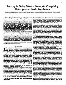
“spray” interchangeably with the term “binary spray” in this article. In SMART, a message may be transmitted using one of the three transmission modes: normal spray mode, companion spray mode and direct transmission mode. A message to be transmitted using normal spray mode will be sprayed to all the nodes that do not have it, whereas a message to be transmitted using companion spray mode is only sprayed to the companions of the destination. And a message to be sent using direct transmission mode will only be forwarded to the destination directly. In the first phase of SMART, the message is sprayed to at most f1 −1 nodes using normal spray mode. If during the first phase the message reaches a companion x of the destination, then in the second phase the companion x uses companion spray mode to spray M to at most f2 − 1 companions of the destination. A node with {M, 1} will use direct transmission mode to send the message to the destination without further forwarding. SMART routing algorithm is showed in Fig. 1. When source S needs to send a message M to a destination D, it checks if it is a companion of D. If so, M is sprayed to at most f2 companions of D. If not, M is sprayed to f1 nodes in the network. When a companion of D receives M , it sprays M only to at most f2 destination’s companions. Fig. 2 illustrates the routing process of SMART. In the example, f1 and f2 is set to be 8 and 4, respectively. We use circle to denote a companion of D and use square to denote a non-companion node. The number in the figure denotes the number of message copies (e.g A(4) means that node A has 4 copies of the message). In this example, the message reaches a companion of D, which sprays the message to other companions of D until the message reaches D. SMART, as a hybrid scheme, combines the strengths of prediction-based schemes and opportunistically-forwarding schemes. It uses Spray algorithm to reach companions quickly and exploits companions to enhance delivery efficiency. The original Spray algorithm controls how many copies of a message are injected into the network but it does not distinguish between nodes and the message is forwarded to every node with equal probability. The SMART’s practice of a companion only spraying to other companions improves routing efficiency by focusing on forwarding the message among the companions of the destination. IV. A NALYSIS OF SMART In this section, we analyze the performance of SMART regarding to message delivery rate and message delivery latency. We use the carriers of a message to denote the nodes that have the message. When a carrier is not a companion of the destination, we call it a generic carrier. Otherwise, we call it a companion carrier. The notations used in the paper are listed in Table I. A. Delivery Rate Analysis Message delivery rate is the percentage of all messages that are delivered to destinations. When analyzing the delivery rate,

Algorithm 1 SMART Routing Input: M , S, D, f1 , f2 if M not sent yet then if S is a companion of D then S stores {M ,⌈f2 /2⌉} and sends {M ,⌊f2 /2⌋} to the first companion of D or D; S uses companion spray mode to send M ; else S stores {M ,⌈f1 /2⌉} and sends {M ,⌊f1 /2⌋} to the first node to meet; S uses normal spray mode to send M ; end if end if if a node y with {M, n} meets a node x without M then y decides whether it forwards M to x based on the transmission mode of M and the value of n; end if if node x receives {M , n} from y for the first time then if x = D then M is delivered and stop; else if x is not a companion of D then if n = 1 then x uses direct transmission mode to send M ; else x stores {M ,⌈n/2⌉} and sends {M ,⌊n/2⌋} to the first node to meet; x uses normal spray mode to send M ; end if else if y is a companion of D then if n = 1 then x uses direct transmission mode to send M ; else x stores {M ,⌈n/2⌉} and sends {M ,⌊n/2⌋} to the first companion to meet; x uses companion spray mode to send M ; end if else x stores {M ,⌈f2 /2⌉} and sends {M ,⌊f2 /2⌋} to the first encoutering companion of D or to D; x uses companion spray mode to send M ; end if end if end if Fig. 1.

SMART routing algorithm S(8)

S(4)

S(2)

S(1)

G(1)

A(4)

B(2)

B(1)

E(1)

A(1)

H(2)

D’s companion normal node

C(2)

A(2)

H(1)

H(4)

C(1)

F(1)

J(2)

J(1)

K(1)

Fig. 2. SMART routing algorithm illustration with f1 = 8 and f2 = 4

TABLE I N OTATIONS Notation CC(t) GC(t) N C(t) N D M γ ξ η α R1 R2 f1 f2 λ

Explanation Number of companion carriers at time t. Number of generic carriers at time t. Number of nodes not having the message at time t. Total number of nodes in the network. Message destination. A message. Maximum number of companions a node can have. Total number of locations in the network. Mobility similarity of the companions. Aging factor. Message propagation rate among generic carriers. Message propagation rate among companion carriers. SMART phase 1 message transmission parameter. SMART phase 2 message transmission parameter. Spray parameter controlling the maximum number of transmissions for a message.

we make the following assumptions: • The nodes move among the locations in the network (e.g. shopping malls, classrooms, restaurants and etc) in discrete steps. A node stays at a location for a period of time then moves to another location. • A node’s location-visiting probabilities are independent and follow uniform distribution. • The time spent on visiting a set of locations is proportional to the size of the set. Nodes exchange messages when they meet at a location. For instance, assume node x have a message for node y. If x’s location visiting sequence is {4, 3, 2 , 1} and y’s location visiting sequence is {2, 3, 1, 4}. Then the messages will be delivered when x and y are both at location 3. Since a message can be either delivered by a generic carrier or a companion carrier, the delivery rate equals (1- probability of generic carriers not meeting the destination - probability of companion carriers not meeting the destination). Equation (5) calculating the delivery rate is based on the above rationale. Now we see the steps of computing equation (5). We use k to denote the number of message carriers (source, companion and generic carriers) and use t to denote time. g First we analyze Pdeliver (k, ξ, t), the cumulative probability of k carriers delivering a message to the destination when the mobility of the message carriers is independent of the destination’s mobility. At any time the destination and k carriers may have ξ k+1 possible location-visiting combinations. g Based on the counting principle, Pdeliver (k, ξ, t) is computed in equation (2).  kt t  ξ(ξ − 1)k ξ−1 g Pdeliver (k, ξ, t) = 1 − (2) = 1 − ξ k+1 ξ Next we compute the delivery probability of a set of c companion carriers meeting the destination. Pdeliver (γ, ξ, η, t) in equation (3) is the cumulative probability of γ companion carriers delivering the message to the destination. Two nodes become companions because they often meet. So we use η to model the mobility similarity of the companions. ηξ represents

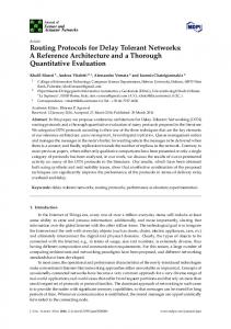
A generic carrier ′may also encounter the destination at the g ηξ locations. So Pdeliver (k, ξ, η, t) in equation (4) calculates the cumulative probability of k generic carriers delivering the message to the destination when they visit the ηξ locations.  ηt ηξ(ξ − 1)k ξ tηk − (ξ − 1)tηk g′ Pdeliver (k, ξ, η, t) = 1− = ηξ × ξ k ξ tηk (4) SMART uses controlled opportunistically-forwarding mechanism so eventually there are f1 generic carriers and f2 companion carriers. The destination and its companions are more likely to encounter at ξη locations, while at the other locations the companions have the same probability as the other nodes to meet the destination. Using equations (2), (3) and (4), equation (5) computes SMART’s message delivery probability. We can see from Fig. 3 that SMART delivers more messages than Spray when f1 + f2 = λ and ξ = 400. Fig.4 shows the delivery rate of SMART increases when η increases from 0.05 to 0.2. Pdeliver (f1 , f2 , ξ, η, t) = g = 1 − [1 − Pdeliver (f1 + f2 , ξ(1 − η), (1 − η)t)] h i g′ c × 1 − Pdeliver (f1 , ξ, η, t) [1 − Pdeliver (f2 , ξ, η, t)] (f1 +f2 )(1−η)t  ξ(1 − η) − 1 =1− ξ(1 − η)  tηf1  f ηt ξ−1 ηξ − 1 2 × (5) ξ ηξ B. Delivery Latency Analysis Message delivery latency measures how long it takes for a message to be delivered to the destination. In this section, we first analyzes the delivery latency of Spray, followed by the delivery latency analysis of SMART. Initially, only the message source has the message. The first phase of SMART is similar to Spray, in which the message is propagated to a number of nodes without differentiating between generic nodes and companions of the destination. In the second phase of SMART, a companion carrier strives to

0.9

SMART (f1=64,f2=4,η=0.05) SMART (f1=64,f2=8),η=0.05) SPRAY (λ=68) SPRAY (λ=72)

0.8

Delivery Rate

0.7

0.6

0.5

0.4

0.3

0.2 2

Fig. 3. 0.9

3

4

5

6 Time

7

8

9

10

Delivery Rate Comparison of SMART and Spray SMART (f1=64,f2=8, η=0.05) SMART (f1=64,f2=8, η=0.1) SMART (f1=64,f2=8, η=0.2)

0.8

0.7 Delivery Rate

the size of the small common location set, where the companions meet. In our assumptions, we assume the time spent on visiting a set of locations is proportional to the size of the set. So γ companion carriers spend ηt visiting ηξ locations. It is worth noting that while the companions visit a set of locations at similar time, their visiting probabilities of the other locations are independent and follow the uniform distribution. Based on c the above analysis, equation (3) calculates Pdeliver (γ, ξ, η, t),  γηt ηξ−1 is the probability of none of γ companion in which ηξ carriers meeting the destination. ηt  (ηξ)(ηξ − 1)γ c Pdeliver (γ, ξ, η, t) = 1 − (ηξ)γ+1  γηt ηξ − 1 = 1− (3) ηξ

0.6

0.5

0.4

0.3

0.2 2

3

Fig. 4.

4

5

6 Time

7

8

9

10

SMART Delivery Rate with Varying η

send the messages to the destination or other companions of the destination. To determine how fast a message is propagated from a generic carrier to other generic nodes and the propagation speed among the companions, we use continuous differential equations to model the message propagations. When we construct differential equations to model message propagation speed, we refer to the principles used in Kermack-McKendrick model [26], a model widely used for modeling epidemic spreading. Without losing generality, in the following analysis, we assume that a source node is a generic node instead of being a companion of the destination. 1) Spray Delivery Latency Analysis: We assume a source node has the same probability as the other nodes to meet the destinations. Therefore, the delivery latency of Spray is determined by the speed of propagating the message to all the nodes in the network. In Spray, the message from the source reaches more and more nodes as time goes on. So GC(t) increases while N C(t) decreases. And we have GC(t) + N C(t) = N.

(6)

In Kermack-McKendrick model, the change of the number of infected hosts is proportional to the product of infection rate, the number of infected hosts and the number of noninfected hosts. Based on this model and equation (6), the change of the number of generic message carriers follows the equation GC(t + ∆t) − GC(t) = R1 × GC(t) × [N − GC(t)]∆t, (7)

where R1 is the message propagation rate from a generic carrier to other generic carriers. Since only the source has the message at the beginning, we have GC(0) = 1. Dividing both sides of equation (7) by ∆t yields the equation (8): dGC(t) = R1 × GC(t) × [N − GC(t)]. (8) dt To solve equation (8), we need to determine R1 . R1 is closely related to ξ and the smaller ξ the larger R1 . So we assume R1 = wξ and conduct simulations using Qualnet Network Simulator [27] to determine w. In the simulations, we set N = 200, λ = N and measure the number of message carriers as time t goes. We run each simulation for 200 times and plot the propagation speed curve using the mean value of 200 simulations. Fig. 5 compares the simulation results and the results obtained by solving equation (8). We find that when R1 = 0.8 ξ , the simulation results match the results obtained by solving (8). Hence, with R1 = 0.8 ξ , we could solve (8) and have the following equation: GC(t) =

N −0.8 Nξt

1−e

+ N e−0.8

(9)

Nt ξ

Since the network we study is large-scale and the number of generic nodes is significantly larger than the number of companions of each node (i.e γ), we can assume the message propagations among the generic nodes and the message propagations among the companions of the destination are independent. Therefore, based on the principles used in constructing equation (8), we derive equation (10) to model the message propagations among the companions. dCC(t) = R2 × CC(t) × [γ − CC(t)] (10) dt R2 , the propagation rate from a companion to other companions, relies on the mobility similarity (i.e ηξ) of the companions. The more frequently two companions meet, the more similar their mobilities are. When N = 200, η = 0.05, γ = 16, f1 = 64, and f2 = 16, we use simulations to find out the value of R2 . Fig. 6 compares the propagation speed among companions obtained from simulations and the propagation speed computed by equation (10). With R2 being set to 0.57 ηξ , the propagation speed computed by equation (10) matches the simulation results very well. 1

1

Spray simulation results R1=0.7/ξ R1=0.8/ξ R1=0.9/ξ

0.9

SMART simulation results SMART R2=0.52/(ηξ) SMART R2=0.57/(ηξ) SMART R2=0.62/(ηξ)

0.8

0.6

0.7 CC(t)/γ

(Number of Message Carriers)/N

0.8

0.6

0.4

0.5 0.4

0.2

0.3 0.2

0

0.1

0

0 0

5

Fig. 5.

10

15

20

25 Time

30

35

40

45

50

R1 vs. Propagation Speed to All Nodes

2) SMART Delivery Latency Analysis: The delivery latency of SMART depends on the speed of propagating the message to the companions of the destination and the speed of propagating the message from one companion to other companions. Therefore, to analyze the delivery latency of SMART, we need to find out the latency from the source to the companions of the destination and the latency from the companions to the destination. The latency from the source to the companions is influenced by f1 and the mobility similarity between the source and the companions, which is largely decided by ξ. When ξ is small or f1 is large, the latency tends to be small and vice versa. Section V-C1 studies the latency from the source to the companions by conducting simulations. From the results of Fig. 8, we find that under our network scenario it takes on average 5 unit time for a message to reach a companion. Here a unit time is 100S, which captures the average time interval between message exchanges in our network scenario. So on average it requires 5 message exchanges for a message to reach a companion of the destination.

Fig. 6.

5

10

15

20

25 Time

30

35

40

45

50

R2 vs. Propagation Speed among Companions

Because on average it takes 5 unit time for a message to reach a companion from the source, we have CC(t) = 0 when 0 ≤ t < 5. Combined with the solution of equation (10), we have ( ) 0, 0 ≤ t < 5 γ CC(t) = (11) 14γt 14γt , t ≥ 5 − − 1−e

ξ

+γe

ξ

Based on equation (9) and (11), Fig. 7 compares the propagation speed of Spray and SMART when N = 200, λ = 200, γ = 16, η = 0.05, f1 = 64 and f2 = 16. The y-axis is the percentage of all nodes reached by Spray (i.e the number of message carriers divided by N ) and the percentage of companions reached by SMART (i.e CC(t)/γ). From Fig. 7, we can see that the message reaches all the companions in SMART before it reaches all nodes in Spray, meaning SMART has smaller delivery latency than Spray. V. E VALUATION A. Performance Comparisons In this section, we evaluate SMART and compare its performance with Spray and Epidemic routing scheme by conducting

TABLE II S IMULATION C ONFIGURATION

Spray SMART

0.8

0.6

0.4

0.2

0 0

Fig. 7.

5

10

15

20

25 Time

30

35

40

45

50

Parameter Number of nodes Terrain dimension Simulation time f1 f2 γ ξ λ of Spray protocol α Mobility model Message traffic model Message Size

Value 200 25600 m×12800 m 1800 S 128 4 or 16 16 400 128 0.98 agenda-based mobility model random (source,destination) pairs 512 bytes

Message Propagation Speed of SMART, Spray

simulations using Qualnet Network Simulator [27]. We focus on comparing the above three routing protocols regarding to the following three metrics. • message delivery rate: This metric measures the percentage of all messages that are delivered to destinations. • message delivery latency: This metric measures on average how long it takes for a message to be delivered. • routing overhead: This metric measures the number of message transmissions per delivered message. In Epidemic routing protocol, a node forwards messages to every node it encounters. Epidemic routing protocol mainly comprises the following two functions. • Beacon propagation: A node periodically broadcasts beacon messages to declare its presence. The beacon message uses a bit vector to specify which messages are now stored on this node. • Message forwarding: When a source has a message to send, it will first check whether the destination is within its radio range. If so, it sends the message to the destination directly. Otherwise, it will forward the message to all nodes encountered, which will further disseminate the message until the message reaches the destination. B. Simulation Setup When evaluating the routing protocol performance, it is important to use a realistic mobility model. As pointed out in many work such as [14], nodes are unlikely to move completely randomly but follow certain mobility patterns. Therefore, we use the agenda mobility model [28] in which nodes follow realistic schedules of activities. The agenda mobility model is supported by realistic user mobility statistics from the National Household Travel Survey [29]. Each activity involves selecting a location from a set of locations, moving to the location selected and staying there for a period of time. There are various types of locations in the terrain, such as schools, working places, gyms, restaurants, homes, shopping malls and so on. And nodes’ visiting patterns to various locations resemble the daily mobility patterns of human beings. The simulation configurations are summarized in table II. For each simulation, we run 5 times (each with a different random seed) and calculate the average value of the results.

C. Results 1) The Configuration of f1 : f1 is one of the important parameters of SMART, which controls the maximum number of message copies injected into the network and affects the number of companion carriers reached at the end of the first phase of SMART. Here we use simulations to study how to configure f1 so that a message will be able to reach a reasonable number of companion carriers at the end of the first phase of SMART. In addition, through simulations we study the latency for a message to reach a companion of the destination. Fig. 8 shows that on average it takes about 5 unit time for a message to reach a companion of the destination. Since the message propagation relies on the message exchanges among nodes, we use 100 seconds as an unit time to capture the average time for exchanging messages between two nodes. Also we let T (a parameter used in CV computation) equal to the simulation time. At the beginning, no companions are reached since it takes some time to spread the message to the nodes. And nodes need some time to accumulate the encounter history. As the time goes on, the dramatic increase of the number of companions reached by the Epidemic routing reflects that the message overhead of Epidemic increases exponentially. Since SMART uses controlled opportunisticallyforwarding mechanism, the number of companions reached by the message stabilizes after all copies of the message are forwarded. 12

SMART f1=32 SMART f1=64 SMART f1=128 Epidemic

10 Num of Companions Reached

Num. Carriers/N of Spray, CC(t)/γ of SMART

1

8

6

4

2

0 0

2

Fig. 8.

4

6 Time (Unit: 100 S)

8

10

Number of Companions Reached vs. f1

650

Epidemic SPRAY (λ=128) SMART (f1=128,f2=4) SMART (f1=128,f2=16)

600

Delivery Latency (seconds)

550

500

450

400

350

300

250 128

Fig. 10.

256

384 Number of Messages

512

640

Delivery Latency vs. Message Traffic

350

Epidemic SPRAY (λ=128) SMART (f1=128,f2=4) SMART (f1=128,f2=16)

300

250 Routing Overhead

2) Performance vs. Traffic Load: In this set of simulations, we vary traffic load (i.e. number of messages sent during the simulation) and measure the aforementioned metrics for the above three routing protocols. Fig. 9 shows the delivery rate when changing message traffic load. The simulation results demonstrate that SMART outperforms Spray protocol and delivers more than 90% messages. The Epidemic routing delivers all the messages since it floods a message to all nodes. The performance of the Spray degrades as traffic load increases because each message has relatively less time to be transmitted when message traffic load increases given that the meeting time between nodes remains the same. But for SMART, the meeting time between nodes has a less significant influence on delivery rate since companions frequently meet each other, thereby having more time to deliver messages to each other. In addition, since message source and destination are randomly selected, the message traffics are more evenly distributed to all nodes when message traffic load increases, which contributes to the slight improvement of SMART’s delivery rate.

200

150

Epidemic SPRAY (λ=128) SMART (f1=128,f2=4) SMART (f1=128,f2=16)

1.02 1

100

50 128

0.98 0.96

Fig. 11.

Delivery Rate

0.94

256

384 Number of Messages

512

640

Routing Overhead vs. Message Traffic

0.92 0.9 0.88 0.86 0.84 0.82 0.8 0.78 0.76 128

256

Fig. 9.

384 Number of Messages

512

640

Delivery Rate vs. Message Traffic

Fig. 10 of the delivery latency demonstrates that SMART has much smaller delivery latency than the Spray. The reason is that SMART exploits companions to deliver the messages while the Spray does not. Because the companions of the destination are more likely to meet the destination, it takes a shorter time for them to deliver the message to the destination. Epidemic routing scheme delivers messages faster than SMART because a node forwards the messages to every node it meets. In this way, the messages are quickly forwarded to the destination. Fig. 11 shows that the routing overhead of Epidemic is much larger than that of SMART and Spray. Epidemic incurs huge overhead because it relies on flooding to deliver messages. SMART and Spray use controlled opportunisticallyforwarding mechanism to forward messages so the number of message transmissions has an upper bound, which is a small constant. It is worth noting that the overhead of SMART and Spray are almost identical when f1 = 4. This is because in SMART after a message reaches a companion, the companion will only forward the message to other companions, which reduces overhead.

3) Performance vs. Mobility: DTN network is a sparse network, which is disconnected most of the time. So message deliveries rely on nodes’ mobility. In different DTN scenarios, nodes’ mobility may vary. A node’s mobility influences the number of locations it may visit during the given simulation time. Hence nodes’ mobility influences the meeting probability of the nodes. In addition, mobility affects meeting time, i.e. how long two nodes stay in each other’s radio range. Higher mobility leads to shorter meeting time. In this set of simulations, we measure the influences of the mobility on the performance of the above three schemes. We alter a node’s mobility by changing its average dwelling time at each location. If we want a node to become more mobile, we decrease its average dwelling time. In the following set of simulations, we vary each node’s average dwelling time at each location from 1 to 5 (normalized against the largest average dwelling time) and fix the message traffic as 256 messages. Fig. 12 demonstrates that when nodes become more mobile, all three routing schemes achieve higher delivery rate. From Fig. 12, we can see that the positive effects on the delivery rate brought by the increase of meeting probability outweighs the negative effects brought by the changes of nodes’ meeting time. Moreover, when nodes become more mobile, the delivery rate of SMART and Spray increasingly approaches that of Epidemic routing. So when nodes have high mobility, we can use SMART to achieve a high delivery ratio with a small routing overhead. Fig. 14 shows that the delivery latency of all three routing

schemes decreases when nodes become more mobile. The reduced latency is because nodes visit more locations in a given time so they have more opportunities to meet and meet each other more quickly. From Fig.13, we know that SMART and Spray maintain a very small routing overhead when mobility changes. Epidemic SPRAY (λ=128) SMART (f1=128,f2=4) SMART (f1=128,f2=16)

1.1

1

Delivery Rate

0.9

0.8

0.7

number of message copies into the network to forward the message to the companions of the destination, which only forward the message to a limited number of the destination’s companions until the message is delivered to the destination. The paper has presented both analytic results and simulation results comparing SMART with the Spray routing scheme and the Epidemic routing scheme. The analytic results demonstrate that SMART has a higher delivery rate and a smaller delivery latency than Spray. And the simulation results show that SMART has a significantly smaller routing overhead than Epidemic while maintaining a comparable delivery rate and delivery latency. From the simulation results, we find that the routing overhead of SMART is almost identical to that of Spray but SMART has a higher delivery rate and a smaller delivery latency.

0.6

R EFERENCES

0.5

0.4 1

1.5

Fig. 12.

2

2.5

3 Node Mobility

3.5

4

4.5

5

Delivery Rate vs. Nodes’ Mobility

350

Epidemic SPRAY (λ=128) SMART (f1=128,f2=4) SMART (f1=128,f2=16)

300

Routing Overhead

250

200

150

100

50 1

1.5

Fig. 13.

2

2.5

3 Node Mobility

800

4

4.5

5

Epidemic SPRAY (λ=128) SMART (f1=128,f2=4) SMART (f1=128,f2=16)

700

Delivery Latency (seconds)

3.5

Routing Overhead vs. Nodes’ Mobility

600

500

400

300

200

100 1

1.5

Fig. 14.

2

2.5

3 Node Mobility

3.5

4

4.5

5

Delivery Latency vs. Nodes’ Mobility

VI. C ONCLUSION The paper has presented a scheme named SMART that exploits controlled opportunistically-forwarding and a node’s companions to achieve efficient message delivery. SMART protocol can achieve high delivery ratio while keeping a low routing overhead. In SMART, a message source injects a fixed

[1] P. Juang, H. Oki, and Y. W. et al., “Energy-Efficient Computing for Wildlife Tracking: Design Tradeoffs and Early Experiences with ZebraNet,” in Proceedings of ASPLOS-X, 2002. [2] A. Doria, M. Udn, and D. P. Pandey, “Providing Connectivity to the Saami Nomadic Community,” in Proc. 2nd Int. Conf. on Open Collaborative Design for Sustainable Innovation, 2002. [3] D. B. Johnson and D. A. Maltz, “Dynamic Source Routing in Ad Hoc Wireless Networks,” in Mobile Computing, 1996, pp. 153–181. [4] C. Perkins and E. Royer, “Ad hoc On-demand Distance Vector Routing,” in 2nd IEEE Workshop on Mobile Computing Systems and Applications, 1999. [5] A. Vahdat and D. Becker, “Epidemic Routing for Partially-connected Ad hoc Networks,” in Technical report, Duke University, 2000. [6] S. Jain, K. Fall, and R. Patra, “Routing in a Delay Tolerant Network,” in ACM Sigcomm, 2004. [7] Y. Wang, S. Jain, M. Martonosi, and K. Fall, “Erasure Coding based Routing in Opportunistic Networks,” in ACM SIGCOMM Workshop on Delay Tolerant Networking, 2005. [8] T. Spyropoulos, K. Psounis, and C. S. Raghavendra, “Single-copy routing in intermittently connected mobile networks,” in Proc. of IEEE Secon’04, 2004. [9] T. Spyropoulos, K. Psounis, and C. Raghavendra, “Spray and wait: an efficient routing scheme for intermittently connected mobile networks,” in WDTN ’05, 2005, pp. 252–259. [10] T. Spyropoulos, K. Psounis, and C. S. Raghavendra, “Spray and focus: Efficient mobility-assisted routing for heterogeneous and correlated mobility,” in PERCOMW ’07, Washington, DC, USA, 2007, pp. 79– 85. [11] A. Lindgren, A. Doria, and O. Schelen, “Probabilistic Routing in Intermittently Connected Networks,” in SIGMOBILE Mobile Computing Communications Review, July 2003, pp. 7:19–20. [12] J. Burgess, B. Gallagher, D. Jensen, and B. Levine, “Maxprop: Routing for vehicle-based disruption-tolerant networking,” in IEEE Infocom, 2006. [13] B. Burns, O. Brock, and B. N. Levine, “MV Routing and Capacity Building in Disruption Tolerant Networks,” in IEEE Infocom, 2005. [14] M. Musolesi, S. Hailes, and C. Mascolo, “Adaptive Routing For Intermittently Connected Mobile Ad hoc Networks,” in WOWMOM’05, 2005. [15] J. Leguay, T. Friedman, and V. Conan, “DTN Routing in a Mobility Pattern Space,” in ACM SIGCOMM - Workshop on delay tolerant networking and related topics (WDTN-05), 2005. [16] J. Ghosh, H. Q. Ngo, and C. Qiao, “Mobility profile based routing within intermittently connected mobile ad hoc networks (icman),” in IWCMC ’06, 2006, pp. 551–556. [17] W. Zhao, M. Ammar, and E. Zegura, “A Message Ferrying Approach for Data Delivery in Sparse Mobile Ad Hoc Networks,” in MobiHoc, 2004. [18] C. Tuduce and T. Gross, “A mobility model based on wlan traces and its validation,” in INFOCOM 2005. IEEE, 2005, pp. 664–674. [19] M. Kim, D. Kotz, and S. Kim, “Extracting a mobility model from real user traces,” in INFOCOM 2006, April 2006.

[20] W. Hsu, T. Spyropoulos, K. Psounis, and A. Helmy, “Modeling timevariant user mobility in wireless mobile networks,” in INFOCOM 2007, Anchorage, Alaska, March 2007. [21] X. Zhang, J. K. Kurose, B. N. Levine, D. Towsley, and H. Zhang, “Study of a bus-based disruption-tolerant network: mobility modeling and impact on routing,” in MobiCom ’07, 2007, pp. 195–206. [22] B. D. Walker, J. K. Glenn, and T. C. Clancy, “Analysis of simple counting protocols for delay-tolerant networks,” in CHANTS ’07, New York, NY, USA, 2007, pp. 19–26. [23] R. Shah, S. Roy, S. Jain, and W. Brunette, “Data MULEs: Modeling a Three-tier Architecture for Sparse Sensor Networks,” in IEEE SNPA, 2003. [24] L. Song and D. F. Kotz, “Evaluating opportunistic routing protocols with large realistic contact traces,” in CHANTS ’07, New York, NY, USA, 2007, pp. 35–42. [25] M. M. B. Tariq, M. Ammar, and E. Zegura, “Message ferry route design for sparse ad hoc networks with mobile nodes,” in MobiHoc ’06, 2006, pp. 37–48. [26] W. Kermack and A. McKendrick, “A contribution to the mathematical theory of epidemics,” in Proceedings of the Royal Society of London Series A, 1927, pp. 700–721. [27] Scalable Network Technologies (SNT), “Qualnet Network Simulator,” http://www.qualnet.com/. [28] Q. Zheng, X. Hong, and J. Liu, “An agenda based mobility model,” in 39th Annual Simulation Symposium, 2006. [29] 2001 national household travel survey, http://nhts.ornl.gov/2001/index.shtml.