Hindawi Publishing Corporation Mathematical Problems in Engineering Volume 2013, Article ID 165927, 6 pages http://dx.doi.org/10.1155/2013/165927
Research Article Message Passing Algorithm for Solving QBF Using More Reasoning Su Weihua, Yin Minghao, Wang Jianan, and Zhou Junping School of Computer Science and Information Technology, Northeast Normal University, Changchun 130117, China Correspondence should be addressed to Wang Jianan;
[email protected] and Zhou Junping;
[email protected] Received 26 June 2013; Accepted 24 July 2013 Academic Editor: William Guo Copyright © 2013 Su Weihua et al. This is an open access article distributed under the Creative Commons Attribution License, which permits unrestricted use, distribution, and reproduction in any medium, provided the original work is properly cited. We present a novel solver for solving Quantified Boolean Formulae problem (QBF). In order to improve the performance, we introduce some reasoning rules into the message passing algorithm for solving QBF. When preprocessing the formulae, the solver incorporates the equality reduction and the hyperbinary resolution. Further, the solver employs the message passing method to obtain more information when selecting branches. By using the unit propagation, conflict driven learning, and satisfiability directed implication and learning, the solver handles the branches. The experimental results also show that the solver can solve QBF problem efficiently.
1. Introduction Quantified Boolean Formulae can be seen as an extension of the well-known canonical NP-complete problem of Propositional Satisfiability (SAT) with existential or universal quantifiers to every variable in the propositional formulae. Given a Quantified Boolean Formula, the question of deciding the satisfiability of the formula is called a Quantified Boolean Satisfiability problem (QBF). QBF is an important issue in artificial intelligence because it is the prototypical PSPACE-complete problem. Many practical problems can be transformed into QBF, for example, conformant planning [1], verification [2], nonmonotonic reasoning [3], and reasoning about knowledge [4]. Now most researchers make great efforts on designing excellent QBF solvers in order to increase the efficiency for solving QBF problem. WalkQSAT is the first incomplete QBF solver using stochastic local search methods, and it applies a SAT solver—walksat for selecting the next branch [5]. WATCHEDCSBJ features watched data structure [6]. QuBE is an adaptation of the classic DPLL (Davis, Putnam, Logemann, and Loveland) backtracking search algorithm. Moreover, it adopts watched data structure and learning [7]. QSAT employs the maximum occurrences in minimum sized clauses (MOMS) heuristic [8]. Quaffle extends variable state independent decaying sum (VSIDS) heuristic and conflict driven learning [9].
In this paper, we propose a novel QBF solver based on a DPLL algorithm, called EHSPQBF. The system combines many advanced techniques together. In preprocessing, we adopt the equality reduction and the hyperbinary resolution to simplify the formulae. In choosing branches process, we employ a message passing method—survey propagation. By giving exact information, the approach selects branches more exactly, which can decrease the search space and improve the backtracking time. In branched treatment process, we utilize conflict reasoning, conflict driven learning, and satisfiability directed implication and learning to help pruning the search space. Owing to these outstanding techniques, the ability of solving QBF problems has greatly improved.
2. Quantified Boolean Formulae We begin this section by presenting some notions in this paper. A literal is either a Boolean variable V or its negation ¬V. If a literal is 𝑙, the negation of the literal is ¬𝑙. A clause is a disjunction of literals which does not contain a complementary pair V and ¬V simultaneously. A propositional logic formula in Conjunction Normal Form (CNF) is a conjunction of clauses. A Quantified Boolean Formula (QBF) has the form 𝑄1 𝑥1 ⋅ ⋅ ⋅ 𝑄𝑛 𝑥𝑛 𝐸 (𝑥1 , 𝑥2 , . . . , 𝑥𝑛 ) ,
(1)
2
Mathematical Problems in Engineering
where 𝐸(𝑥1 , 𝑥2 , . . . , 𝑥𝑛 ) is a propositional logic formula in CNF involving Boolean variables 𝑥1 , 𝑥2 , . . . , 𝑥𝑛 , and every 𝑄𝑖 (1 ≤ 𝑖 ≤ 𝑛) is either an existential quantifier ∃ or a universal quantifier ∀. A variable is existential if the restriction quantifier of the variable is ∃, and universal otherwise. Any Boolean variable V can take a value true or false. A truth assignment for a propositional logic formula is a map that assigns each variable a value. The satisfying assignment, called model, is the truth assignment that makes the propositional logic formula evaluated to true. The partial variable assignment is a map that assigns some variables values. We say a formula composed of zero clause is an empty formula, denoted by 𝐸 = ⌀, which is interpreted as true. An empty clause is a clause containing zero literal, which means that the clause is false. The Quantified Boolean Formulae Satisfiability problem is to decide whether a Quantified Boolean Formula is satisfiable. For example, given a QBF ∀𝑥1 ∃𝑥2 ((𝑥1 ∨ 𝑥2 ) ∧ (¬𝑥1 ∨ ¬𝑥2 )), the QBF is satisfiable if and only if for each truth assignment to 𝑥1 there exists a truth assignment to 𝑥2 . In the rest of the paper, we will use QBF to denote the formulae and the satisfiability problems. For a QBF of the form (1), because ∃𝑥1 ∃𝑥2 𝐸(𝑥1 , 𝑥2 ) ≡ ∃𝑥2 ∃𝑥1 𝐸(𝑥1 , 𝑥2 ) and ∀𝑥1 ∀𝑥2 𝐸(𝑥1 , 𝑥2 ) ≡ ∀𝑥2 ∀𝑥1 𝐸(𝑥1 , 𝑥2 ), we can group in the same set all consecutive variables having the same quantifier. Therefore, equality (1) can be rewritten into the following form: 𝑄1 𝑋1 ⋅ ⋅ ⋅ 𝑄𝑘 𝑋𝑘 𝐸 (𝑥1 , 𝑥2 , . . . , 𝑥𝑛 )
(1 ≤ 𝑘 ≤ 𝑛) ,
(2)
where 𝑋𝑖 (1 ≤ 𝑖 ≤ 𝑘) is a set of propositional variables and all such sets are mutual disjoint. In such a format, each quantifier is applied to a set of variables rather than to a single Boolean variable. Moreover, the sequence of quantifiers alternates; an existential quantifier follows a universal quantifier and vice versa. With the quantifier restricted, each variable has a quantification level, which increases from the outermost quantification set to the innermost quantification set; that is, the variables belonging to the outermost quantification set have quantification level 1 and so forth.
3. The Relationship between SAT and QBF The SAT problem is a typical NP-complete problem, which has a close relationship with QBF problem. More specifically, SAT can be regarded as an especial form of QBF with only existing existential quantifier, and QBF can be regarded as an extended form of SAT with additional prefixes. In addition, they are both prototypical problems for complexity classes. SAT is an NP-complete problem while QBF is a PSPACEcomplete problem, which is inherently more difficult than SAT. In the following, we will discuss the similarities and dissimilarities between QBF and SAT. Orders of Disposing Variables. When dealing with SAT, we can select variables in a random order. While dealing with QBF, we must select variables in a sequence of quantifier level that is, the variables whose quantifier level is minimal will be assigned first and so on. As a matter of fact, the reason
of doing so is that the variables in QBF have a dependency relationship. For example, given a QBF ∀𝑥1 ∃𝑥2 ((𝑥1 ∨ 𝑥2 ) ∧ (¬𝑥1 ∨ ¬𝑥2 )), the value of an existential 𝑥2 that makes the formula true may depend directly on the value of a universal 𝑥1 which is quantified prior to 𝑥2 . Therefore, the key of dealing with QBF is to select the variables in the sequence of quantifier level. Search Space. The search space of SAT is a tree while the search space of QBF is an AND/OR tree. They both regard the assignment of variables as weights and variables as nodes. The difference is that QBF has two types of nodes: AND node and OR node. In the AND/OR tree, the universal variables correspond to the AND nodes and the existential variables correspond to the OR nodes. Hardness of the Problems. The QBF is more difficult than SAT. As we know, SAT is NP-complete while QBF is PSPACEcomplete. For a SAT, the algorithm will stop when a satisfying assignment is found. However, for a QBF, the algorithm needs to continue searching because of the universal quantifiers. Because of the close relationship between SAT and QBF, most of methods for QBF can be regarded as a generalization of algorithms commonly for SAT. Therefore, we can solve QBF with equality reduction and the hyperbinary resolution which is really effective in solving SAT.
4. QBF Algorithm Framework Recently, search-based QBF solvers are based on an extension to the DPLL algorithm. Now we give the DPLL algorithm for QBF in Algorithm 1. In the algorithm, 𝐶⌀ is an empty clause and 𝐶all∀ is a clause composed of only universal variables. The DPLL algorithm works on the principle of preprocessing, choosing branches, branched treatment, and then recursively solving the simplified QBF. In preprocessing process (line 1), DPLL employs several reasoning rules to simplify QBF like pure literal rule, unit literal rule, and so forth. In choosing branches (variables) process (line 4), DPLL selects variables in a fixed order; that is, the variables in the outermost quantification set are chosen first and so on. In branched treatment process (lines 5–8), DPLL searches AND/OR tree depending on the chosen variable. If the chosen variable is an existential variable, an OR node is explored; otherwise an AND node is explored. DPLL terminates when the simplified QBF is an empty formula (line 2), which means the input formula 𝑄 ⋅ 𝐸 is satisfiable; when the simplified QBF contains an empty clause or there is a clause made of all universally quantified variables (line 3), which means the input formula 𝑄 ⋅ 𝐸 is unsatisfiable. In Algorithm 2, we present the basic algorithm of EHSPQBF, which is based on DPLL algorithm. At first, we explain the terms occurred in the algorithm. The term 𝐶⌀ is an empty clause, and 𝐶all∀ is a clause composed of only universal variables. In preprocessing process (line 1), we simplify the input formula in CNF employing unit literal rule, the equality reduction, and the hyperbinary resolution. In choosing branches process (line 9), we use survey propagation as a heuristic. By giving exact information,
Mathematical Problems in Engineering
3
Procedure DPLL (𝑄 ⋅ 𝐸) (1) preprocess (𝑄 ⋅ 𝐸); (2) if 𝐸 = ⌀ then return SAT; (3) if (𝐶⌀ ∈ 𝐸) ∨ (𝐶all∀ ∈ 𝐸) then return UNSAT; (4) V ← choosevariable (𝑄 ⋅ 𝐸); (5) if (V is existential) (6) then return DPLL ( 𝑄 ⋅ 𝐸|V=true ) or DPLL (𝑄 ⋅ 𝐸|V=false ) (7) if (v is universal) (8) then return DPLL (𝑄 ⋅ 𝐸|V=true ) and DPLL (𝑄 ⋅ 𝐸|V=false ) Algorithm 1: DPLL for solving QBF.
Procedure EHSPQBF (𝑄 ⋅ 𝐸) (1) preprocess (𝑄 ⋅ 𝐸); (2) if (𝐸 = ⌀) then return SAT; (3) if (𝐶⌀ ∈ 𝐸) ∨ (𝐶all∀ ∈ 𝐸) then return UNSAT; (4) result = deduce(); (5) if (result = conflict) (6) then analyze conflict(); (7) if (result = satisfaction) (8) then analyze satisfaction(); (9) V ← SP choosevariable (𝑄 ⋅ 𝐸); (10) if (V is existential) (11) then return EHSPQBF (𝑄 ⋅ 𝐸|V=true ) or EHSPQBF (𝑄 ⋅ 𝐸|V=false ) (12) if (v is universal) (13) then return EHSPQBF (𝑄 ⋅ 𝐸|V=true ) and EHSPQBF (𝑄 ⋅ 𝐸|V=false ) Algorithm 2: EHSPQBF algorithm.
the approach makes the choice of branch more exactly, which can decrease the search space and improve the runtime. In branched treatment process (line 4), we deduce the formula using conflict reasoning rule. The result of the deduction has three values: undetermined, satisfaction, and conflict. If result is conflict (satisfaction), that is, 𝐸 evaluates to 0 (resp., 1) under the current partial variable assignment, the algorithm analyzes the conflict (resp., satisfaction); if the result is undetermined, that is, 𝐸 evaluates neither 0 nor 1, the algorithm continues to choose branches. In this process, we employ the conflict driven learning and satisfiability directed learning to reduce the search space.
5. Preprocessing via Reasoning Rules Besides the unit literal rule, the preprocess stage also uses more powerful reasoning rules, that is, the hyperbinary resolution and the equality reduction [10]. As a matter of fact, the hyperbinary resolution rule is a sequence of ordinary resolution steps. Though they are of similar function in simplifying the formulae, the hyperbinary resolution reduces the space which the sequence intermediate clauses occupy. And the equality reduction rule can further reduce the size of the input formula. It first finds the equivalences, and then it substitutes each equivalent variable, which can simplify the input formula. Now we describe them in the following.
Definition 1. The hyperbinary resolution rule of inference takes as input a 𝑚 + 1-ary clause (𝑙1 ∨ 𝑙2 ∨ ⋅ ⋅ ⋅ ∨ 𝑙𝑚 ∨ 𝑙) and 𝑚 binary clauses each of the form (¬𝑙𝑖 ∨ 𝑙 ) (1 ≤ 𝑖 ≤ 𝑚), where 𝑙𝑖 (1 ≤ 𝑖 ≤ 𝑚) is existential variable; then it deduces the clause (𝑙 ∨ 𝑙 ). The advantage of the hyperbinary resolution is that it can save the solving time. The hyperbinary resolution can generate unit clauses or binary clauses in order to simplify the input formula. In addition, if the deduced clause contains only universal variables, the formula can be directly decided the QBF instance is unsatisfiable. For example, consider a formula 𝐹 = ∀𝑥∃𝑥1 𝑥2 𝑥3 𝑥4 𝑥5 𝑥6 (𝑥1 ∨ 𝑥) ∧ (𝑥2 ∨ 𝑥) ∧ (𝑥3 ∨ 𝑥) ∧ (𝑥4 ∨𝑥)∧(𝑥5 ∨𝑥)∧(𝑥6 ∨𝑥)∧(¬𝑥1 ∨¬𝑥2 ∨¬𝑥3 ∨¬𝑥4 ∨¬𝑥5 ∨¬𝑥6 ). If we apply the hyperbinary resolution rule to 𝐹, the rule is able to obtain a deduced clause 𝑥 which contains only one universal variable, and we can decide that the formula is unsatisfiable. By simplifying the formula, the hyperbinary resolution rule reduces the solving time. Definition 2. The equality reduction of a QBF formula 𝐹 by a pair of equivalent literals 𝑙1 ≡ 𝑙2 is a rule of replacing 𝑙1 by 𝑙2 if 𝐹 satisfies (1) 𝐹 contains the pair of binary clauses (¬𝑙1 ∨𝑙2 ) and (𝑙1 ∨ ¬𝑙2 ); (2) the quantification level of 𝑙1 is greater than 𝑙2 ; (3) 𝑙1 and 𝑙2 are both existential.
4
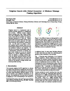
Mathematical Problems in Engineering graph in Figure 1, where clause 𝑎 represents 𝑥1 ∨𝑥2 and clause 𝑏 represents ¬𝑥1 ∨ ¬𝑥2 .
1 b
a
2
Figure 1: A simple example of a factor graph.
Note that the QBF formula 𝐹 is unsatisfiable if there is a universal in the clause ¬𝑙1 ∨ 𝑙2 . Once that equality reduction finds the equivalences, then it substitutes each variable with its definition in the formula. For example, let 𝐹 = ∃𝑥1 ∀𝑥3 𝑥4 ∃𝑥2 (𝑥1 ∨ ¬𝑥2 ) ∧ (¬𝑥1 ∨ 𝑥2 ) ∧ (𝑥1 ∨ ¬𝑥2 ∨ 𝑥3 ) ∧ (𝑥2 ∨ ¬𝑥4 ) ∧ (𝑥1 ∨ 𝑥2 ∨ 𝑥4 ). Since literals 𝑥1 and 𝑥2 are equivalent literals, we obtain the simplified QBF. 𝐹 is ∃𝑥1 ∀𝑥4 (𝑥1 ∨ ¬𝑥4 ) ∧ (𝑥1 ∨ 𝑥4 ) by using equality reduction. Notice that when the hyperbinary resolution rule applies to 𝐹 , the input formula can be further simplified. Above all, we can find that the hyperbinary resolution rule and equality reduction have the power to reduce the size of the formula. They cannot only occupy less space but also increase the efficiency for solving QBF.
6. Choosing Branches with Survey Propagation The survey propagation (SP) [11] method is a groundbreaking development for solving SAT. The occurrence makes the SAT problems that we can deal with scale from with ten thousand variables to with one million variables. As far as we know, SP is the only algorithm successful at solving random SAT problems with one million variables and beyond in near-linear time in the hardest region. In this section, we will discuss how to choose branches with the SP method. As a message passing algorithm, SP passes message on a factor graph which provides an easy graphical description to the message passing procedures. In the following, we will address the factor graph in detail. 6.1. Factor Graph. The factor graph is an undirected graph (see Figure 1). It has two types of nodes: one represents variables called “variable node” (circles in Figure 1) and the other represents clauses called “function node” (squares in Figure 1). A function node 𝑎 is connected to a variable node 𝑖 by an edge whenever the variable 𝑖 (or its negation) appears in the clause 𝑎. In the graphical representation, we use a full (dashed) line between 𝑎 and 𝑖 whenever the variable appearing in the clause is 𝑖 (¬𝑖). For every variable node 𝑖, we denote by 𝑉(𝑖) the set of function nodes to which it is connected, by 𝑉+ (𝑖) the subset of consisting of function nodes where the variable appears unnegated, and by 𝑉− (𝑖) the complementary set of 𝑉+ (𝑖). V(𝑖) \ 𝑏 denotes the set V(𝑖) without node 𝑏. Similarly, for each function node 𝑎, we denote by 𝑉(𝑎) = 𝑉+ (𝑎)∪𝑉− (𝑎) the set of neighboring variable nodes. For example, given a QBF ∀𝑥1 ∃𝑥2 (𝑥1 ∨ 𝑥2 ) ∧ (¬𝑥1 ∨ ¬𝑥2 ), we can represent the propositional logic formula with factor
6.2. Message Passing. The survey propagation algorithm passes two types of messages: one passed from a function node to a variable node; the other passed from a variable node to a function node. The update of both messages is realized by the message update rule which is defined as follows. (1) The message passed from a function node 𝑎 to a variable node 𝑖: the message, called “survey”, is a real number 𝜂𝑎 → 𝑖 𝜖 [0, 1]: 𝜂𝑎 → 𝑖 = ∏ [ 𝑗∈𝑉(𝑎)\𝑖
Π𝑢𝑖→ 𝑎
Π𝑢𝑖→ 𝑎 ]. + Π𝑠𝑖 → 𝑎 + Π0𝑖→ 𝑎
(3)
If 𝑉(𝑎) \ 𝑖 is empty, then 𝜂𝑎 → 𝑖 = 1. In equality (3), the variable 𝑗 sends a particular symbol to clause 𝑎 saying that the variable cannot satisfy the clause (“𝑢”), that the variable can satisfy the clause (“𝑠”), or that it is indifferent (“0”). (2) The message passed from a variable node 𝑖 to a function node 𝑎: each variable 𝐼 ∈ 𝑉 passes a triplet of real numbers Π𝑖 → 𝑎 = (Π𝑢𝑖→ 𝑎 , Π𝑠𝑖 → 𝑎 , Π0𝑖→ 𝑎 ) to each of its clause neighbors 𝑎 ∈ 𝑉(𝑖): Π𝑢𝑖→ 𝑎 = [1 − ∏ (1 − 𝜂𝑏 → 𝑖 )] ∏ (1 − 𝜂𝑏 → 𝑖 ) , 𝑠 𝑏∈𝑉𝑎𝑢 (𝑖) [ ] 𝑏∈𝑉𝑎 (𝑖) Π𝑠𝑖 → 𝑎 = [1 − ∏ (1 − 𝜂𝑏 → 𝑖 )] ∏ (1 − 𝜂𝑏 → 𝑖 ) , 𝑢 𝑏∈𝑉𝑎𝑠 (𝑖) [ ] 𝑏∈𝑉𝑎 (𝑖)
(4)
Π0𝑖→ 𝑎 = ∏ (1 − 𝜂𝑏 → 𝑖 ) , 𝑏∈𝑉(𝑖)\𝑎
where V𝑎𝑢 (𝑖) and V𝑎𝑠 (𝑖) denote neighbors which tend to make variable 𝑖 dissatisfy or satisfy clause 𝑎. If a set like V𝑎𝑠 (𝑖) is empty, the corresponding product takes value 1. In the above equalities, the variable 𝑖 sends a particular symbol to clause 𝑎 saying that the variable cannot satisfy the clause (“𝑢”), that the variable can satisfy the clause (“𝑠”), or that it is indifferent (“0”). When SP converges to a fixed point set of messages 𝜂𝑎∗→ 𝑖 , one can use it to estimate the statistic characteristic (called bias) of every variable. There are two types of biases: positive bias and negative bias. The positive (negative) bias is the probability that variable 𝑖 is restricted to 1 (0). The computing formulae are as follows: 𝑊𝑖(+) = 𝑊𝑖(−)
̂+ Π 𝑖 , + ̂ ̂ ̂0 Π + Π− + Π 𝑖
𝑖
𝑖
̂− Π 𝑖 = + , ̂ +Π ̂− + Π ̂0 Π 𝑖
𝑖
𝑖
(5)
Mathematical Problems in Engineering
5
where ̂+ Π 𝑖
= [1 − ∏ (1 − 𝑎∈𝑉+ (𝑖) [
𝜂𝑎∗→ 𝑖 )]
∏ (1 − ] 𝑎∈𝑉− (𝑖)
𝜂𝑎∗→ 𝑖 ) ,
̂ − = [1 − ∏ (1 − 𝜂∗ )] ∏ (1 − 𝜂∗ ) , Π 𝑖 𝑎→𝑖 𝑎→𝑖 𝑎∈𝑉− (𝑖) [ ] 𝑎∈𝑉+ (𝑖)
(6)
Routine analyze conflict() (1) conflictcl = find conflict clause(); (2) newcl = gen clause (conflict cl); (3) add clause (new cl); (4) if (dl (new cl) ≠ 0) (5) then backtrack (dl(new cl)); (6) end
̂ 0 = ∏ (1 − 𝜂∗ ) . Π 𝑖 𝑎→𝑖
Algorithm 3: Analyze conflict routine.
As a whole, SP gathers the statistical information which can guide the choosing branches. In choosing branches process, we select branches obeying quantification orders. For variables in the same quantification level, we compute positive and negative biases with SP. Then we fix the biased variable in the same quantification level; that is, one variable has the largest bias |𝑊𝑖(+) −𝑊𝑖(−) |. Having selected the variable, we assign the variable depending on the current quantification level. If the current quantification level is existential, we assign the biased value to the variable; otherwise we assign the reverse biased value to the variable.
Routine analyze SAT() (1) entity = find sat entity(); (2) if (entity = NULL) (3) then entity = gen sat induced entity(); (4) if (!termnate condition (entity)) (5) then newen = consensus gen entity (entity); (6) add newentity (newen); (7) if (dl (newen) ≠ 0) (8) then backtrack (dl (newen)); (9) end
𝑎∈𝑉(𝑖)
Algorithm 4: Analyze SAT routine.
7. Branched Treatment After choosing branches, we can perform branched treatment on the chosen variable. The purpose of treatment is to decide whether the current branch of search tree is satisfiable. In branched treatment process, we employ some efficient technologies, such as conflict reasoning, conflict driven learning, and satisfiability directed learning. 7.1. Conflict Driven Learning. Conflict driven learning utilizes the knowledge learned from failures in certain search space to help prune search in future spaces. If the current branch of the search tree is not satisfied, we can perform conflict driven learning. It is carried out by the analyze conflict routine in Algorithm 3. The analyze conflict routine analyzes the current status and brings the search to a new space by backtracking. At first, we explain some terms in the routine. As an algorithm based on DPLL, EHSPQBF is a branch and search procedure. Each branch has a decision level (𝑑𝐿). The first branch has decision level 1 and so forth. And variables implied by a decision variable will have the same decision level as the decision variable. Now we introduce the analyze conflict routine. At the beginning, it decides whether there exist conflict clauses in the current QBF formula (line 1). If they exist, we utilize function gen clause() for generating learned clause (line 2). The learned clause can guarantee that the decision level which the algorithm backtracks to is unique. Then function add clause() performs conflict driven learning when the result of deduction is conflict, which causes a learned clause constructed and added to the database (line 3). At last, we decide whether the decision level that the algorithm backtracks to 0 (line 4). If it is not 0, EHSPQBF will backtrack to the decision level (line 5). The aim of conflict driven learning is to memorize the conflict branch. If search
space has the same branch in the further, we can prune the branch directly, which need not go on searching. 7.2. Satisfiability Directed Learning. Satisfiability directed learning utilizes the knowledge learned from satisfactions to reduce the number of satisfying leaves which need to be visited. When the result of deduction is satisfaction, we can perform satisfiability directed learning. It is carried out by the analyze SAT routine in Algorithm 4. At first, we show relevant definitions used in the routine. Definition 3. (extended CNF) Let 𝐸(𝑥1 , . . . , 𝑥𝑛 ) be a CNF. An extended CNF is 𝐸 = 𝐸(𝑥1 , . . . , 𝑥𝑛 ) ∨ 𝐸𝑁1 ∨ . . . ∨ 𝐸𝑁𝑚 , where 𝐸𝑁𝑖 (1 ≤ 𝑖 ≤ 𝑚) is an entity, that is, a conjunction of literals. Now let us introduce the detail of the routine. At the beginning, it judges whether there exist satisfying entities in the current QBF in extended CNF (line 1). If they exist, the routine goes to line 4; otherwise, 𝑎 entity from the current variable assignment is generated by function gen sat induced entity() (lines 2-3). In lines 4-5, a learned entity is not generated by function consensus gen entity() until the generated entity meets the following conditions. (1) Among all its universal variables, one and only one has the highest decision level, supposing the variable is 𝑉; (2) 𝑉 is at a decision level with a universal variable as the decision variable; (3) all existential literals with quantification level smaller than 𝑉’s are assigned true before 𝑉’s decision level. The decision level of universal variable 𝑉 is the decision level which the algorithm will backtrack to. Then function add newentity() performs satisfiability directed learning (line 6). It occurs when the result of deduction is satisfaction, which causes a learned entity constructed and added to the database. At last, we decide whether the decision level of variable 𝑉 is
6
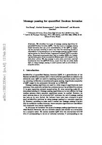
Mathematical Problems in Engineering Table 1: Comparisons of EHSPQBF-EQR, EHSPQBF-HBR, and EHSPQBF.
Instances (3, 60, 80, 5, 0) (3, 60, 80, 5, 1) (3, 60, 80, 5, 2) (3, 60, 80, 5, 3) (3, 60, 80, 5, 4) (3, 60, 80, 5, 5)
EHSPQBF-EQR 10.470 56.342 230.230 1.783 98.456 12.479
EHSPQBF-HBR 15.390 41.230 153.690 3.467 132.678 30.745
EHSPQBF 10.209 40.725 153.436 1.659 87.513 11.873
0 or not (line 7). If it is not 0, EHSPQBF will backtrack to the decision level of variable 𝑉 (line 5). The aim of satisfiability directed learning is memorizing the satisfied branch. If search space has the same branch in the further, we can decide the branch is satisfiable directly and go on searching the other branch of the universal variable.
Universities (Grant no. 11QNJJ006), the Ministry of Education (Grant no. 20120043120017), the Postdoctoral Science Foundation of China (2012M520658), and the opening fund of top key discipline of computer software and theory in Zhejiang provincial colleges at Zhejiang Normal University (Grant no. ZSDZZZZXK37).
8. Experimental Evaluation
References
In this section, to test the performance of the solver EHSPQBF, three algorithms are compared. Our solver EHSPQBF is written in C++. All experiments are carried out on a DELL PowerEdge 2650 computer with 2 Intel Xeon 2.00 GHz CPU and 1G RAM running RedHat ES3.0. Table 1 presents the results of the comparisons of the solvers. In the table, EHSPQBF-HBR is the solver that removes the hyperbinary resolution rule from EHSPQBF; EHSPQBFEQR is the solver that removes the equality reduction rule from EHSPQBF. All instances are generated by a random generator. (3, 60, 80, 5, 0) denotes a formula indexing 0 that contains 3 quantification levels, 60 variables, 80 clauses, and each clause length is not more than 5. From the results of the EHSPQBF, we can see that both hyperbinary resolution rule and equality reduction rule contribute much compared with the results of EHSPQBFEQR and EHSPQBF-HBR. Consequently the run-time of the algorithms decreases. Therefore, by introducing the hyperbinary resolution rule and equality reduction rule, EHSPQBF algorithm increases the efficiency for solving QBF problem.
[1] J. Rintanen, “Asymptotically optimal encodings of conformant planning in QBF,” in Proceedings of the 22nd AAAI Conference on Artificial Intelligence, pp. 1045–1050, July 2007. [2] P. Marin, C. Miller, and B. Becker, “Incremental QBF preprocessing for partial design verification,” in Proceeding of the 15th International Conference of Theory and Applications of Satisfiability Testing, pp. 473–474, 2012. [3] U. Egly, T. Eiter, H. Tompits, and S. Woltran, “Solving advanced reasoning tasks using quantified Boolean formulas,” in Proceeding of the 12th AAAI Conference on Artificial Intelligence, pp. 417– 422, 2000. [4] G. Pan and M. Y. Vardi, “Optimizing a BDD-based modal solver,” in Proceedings of the 19th International Conference on Automated Deduction, pp. 75–89, August 2003. [5] I. P. Gent, H. H. Hoos, A. G. D. Rowley, and K. Smyth, “Using stochastic local search to solve quantified Boolean formulae,” in Proceeding of the Principles and Practice of Constraint Programming, pp. 348–362, 2003. [6] I. Gent, E. Giunchiglia, M. Narizzano, A. Rowley, and A. Tachella, “Watched data structures for QBF solvers,” in Proceeding of the 6th International Conference on Theory and Applications of Satisfiability Testing, pp. 348–355, 2003. [7] E. Giunchiglia, M. Narizzano, and A. Tacchella, “QuBE: a system for deciding quantified Boolean formulas satisfiability,” in Proceeding of the 17th International Joint Conference on Artificial Intelligence, pp. 18–23, 2001. [8] J. Rintanen, “Partial implicit unfolding in the Davis Putnam procedure for quantified Boolean formulae,” in Proceeding of the 8th International Conference on Logic for Programming, Artificial Intelligence and Reasoning, pp. 362–376, 2001. [9] L. Zhang and S. Malik, “Towards a symmetric treatment of satisfaction and conflicts in quantified Boolean formula evaluation,” in Proceeding of the Principles and Practice of Constraint Programming, pp. 200–215, 2002. [10] F. Bacchus, “Enhancing Davis Putnam with extended binary clause reasoning,” in Proceedings of the 18th National Conference on Artificial Intelligence (AAAI ’02), pp. 613–619, August 2002. [11] M. M´ezard, G. Parisi, and R. Zecchina, “Analytic and algorithmic solution of random satisfiability problems,” Science, vol. 297, no. 5582, pp. 812–815, 2002.
9. Conclusions In this paper, we present a novel QBF solver EHSPQBF. In preprocessing, we adopt the equality reduction and the hyperbinary resolution to simplify the formulae. When choosing branches, the system uses survey propagation to select next branch; when handling branches, the system employs conflict reasoning and conflict driven learning as well as satisfiability directed learning together. Experimental results show that, as a heuristic, SP can choose branches effectively. And other techniques such as conflict driven learning also speed up the solving process. As a whole, EHSPQBF is an efficient QBF solver.
Acknowledgments This work was fully supported by the National Natural Science Foundation of China (Grant nos. 11226275, 61103136, and 61070084), the Fundamental Research Funds for the Central
Advances in
Operations Research Hindawi Publishing Corporation http://www.hindawi.com
Volume 2014
Advances in
Decision Sciences Hindawi Publishing Corporation http://www.hindawi.com
Volume 2014
Journal of
Applied Mathematics
Algebra
Hindawi Publishing Corporation http://www.hindawi.com
Hindawi Publishing Corporation http://www.hindawi.com
Volume 2014
Journal of
Probability and Statistics Volume 2014
The Scientific World Journal Hindawi Publishing Corporation http://www.hindawi.com
Hindawi Publishing Corporation http://www.hindawi.com
Volume 2014
International Journal of
Differential Equations Hindawi Publishing Corporation http://www.hindawi.com
Volume 2014
Volume 2014
Submit your manuscripts at http://www.hindawi.com International Journal of
Advances in
Combinatorics Hindawi Publishing Corporation http://www.hindawi.com
Mathematical Physics Hindawi Publishing Corporation http://www.hindawi.com
Volume 2014
Journal of
Complex Analysis Hindawi Publishing Corporation http://www.hindawi.com
Volume 2014
International Journal of Mathematics and Mathematical Sciences
Mathematical Problems in Engineering
Journal of
Mathematics Hindawi Publishing Corporation http://www.hindawi.com
Volume 2014
Hindawi Publishing Corporation http://www.hindawi.com
Volume 2014
Volume 2014
Hindawi Publishing Corporation http://www.hindawi.com
Volume 2014
Discrete Mathematics
Journal of
Volume 2014
Hindawi Publishing Corporation http://www.hindawi.com
Discrete Dynamics in Nature and Society
Journal of
Function Spaces Hindawi Publishing Corporation http://www.hindawi.com
Abstract and Applied Analysis
Volume 2014
Hindawi Publishing Corporation http://www.hindawi.com
Volume 2014
Hindawi Publishing Corporation http://www.hindawi.com
Volume 2014
International Journal of
Journal of
Stochastic Analysis
Optimization
Hindawi Publishing Corporation http://www.hindawi.com
Hindawi Publishing Corporation http://www.hindawi.com
Volume 2014
Volume 2014