Message Passing Algorithms - People

Universit¨ at des Saarlandes Max-Planck-Institut f¨ ur Informatik

Message Passing Algorithms Masterarbeit im Fach Informatik Masters Thesis in Computer Science von / by

Megha Khosla angefertigt unter der Leitung von / supervised by

Prof. Dr. Kurt Melhorn betreut von / advised by

Dr. Konstantinos Panagiotou begutachtet von / reviewers

Prof. Dr. Kurt Melhorn Dr. Konstantinos Panagiotou

December 2009

Declaration of Authorship I, Megha Khosla, declare that this thesis titled, ‘Message Passing Algorithms’ and the work presented in it are my own. I confirm that:

This work was done wholly or mainly while in candidature for a Masters degree at this University.

Where I have consulted the published work of others, this is always clearly attributed.

Where I have quoted from the work of others, the source is always given. With the exception of such quotations, this thesis is entirely my own work.

I have acknowledged all main sources of help.

Where the thesis is based on work done by myself jointly with others, I have made clear exactly what was done by others and what I have contributed myself.

Signed:

Date:

i

Abstract Constraint Satisfaction Problems (CSPs) are defined over a set of variables whose state must satisfy a number of constraints. We study a class of algorithms called Message Passing Algorithms, which aim at finding the probability distribution of the variables over the space of satisfying assignments. These algorithms involve passing local messages (according to some message update rules) over the edges of a factor graph constructed corresponding to the CSP. We focus on the Belief Propagation (BP) algorithm, which finds exact solution marginals for tree-like factor graphs. However, convergence and exactness cannot be guaranteed for a general factor graph. We propose a method for improving BP to account for cycles in the factor graph. We also study another message passing algorithm known as Survey Propagation (SP), which is empirically quite effective in solving random K − SAT instances, even when the density is close to the satisfiability threshold. We contribute to the theoretical understanding of SP by deriving the SP equations from the BP message update rules.

Acknowledgements I would like to thank Prof. Kurt Melhorn for giving me the opportunity to pursue this thesis under his supervision and his timely and valuable inputs. I am grateful to my advisor, Konstantinos Panagiotou for bringing an interesting and challenging research topic to my attention. I also thank him for his persistent support and patience through many discussions we had through the course of the thesis. He has been an excellent advisor. I thank my parents for being a source of continued emotional support and teaching me to aim high. I am thankful to all my friends for their support and encouragement.

iii

Contents Declaration of Authorship

i

Abstract

ii

Acknowledgements

iii

List of Figures

vi

1 Introduction 1.1 Summary of Contributions . . . . . . . . . . . . . . . . . . . . . . . . . . . 1.2 Organization . . . . . . . . . . . . . . . . . . . . . . . . . . . . . . . . . . 2 Preliminaries 2.1 Constraint Satisfaction Problems . . . . . . . . . . . . . . . 2.2 Graphical Models . . . . . . . . . . . . . . . . . . . . . . . . 2.2.1 Conditional Independence and Markovian Properties 2.2.2 Factor Graphs . . . . . . . . . . . . . . . . . . . . . 2.3 Exploiting Structure for Efficient Computations . . . . . . . 3 Belief Propagation 3.1 Introduction . . . . . . . . . . . . . . . . . . . . . . . 3.2 Beliefs and Message Equations . . . . . . . . . . . . 3.3 Belief Propagation for Trees . . . . . . . . . . . . . . 3.4 Loopy Belief Propagation for General Graphs . . . . 3.4.1 Conditioning/Clamping for Exact Marginals . 3.4.2 Exact BP Algorithm for General Graphs . . . 4 Properties of Loopy Belief Propagation 4.1 Introduction . . . . . . . . . . . . . . . . . . . . . . . 4.2 Fixed Points of BP . . . . . . . . . . . . . . . . . . . 4.3 Generalized Belief Propagation . . . . . . . . . . . . 4.4 Correctness of Loopy BP for some Graphical Models

. . . . . . . . . .

. . . . . . . . . .

. . . . . . . . . .

. . . . . . . . . .

. . . . . . . . . . . . . . .

. . . . . . . . . . . . . . .

. . . . . . . . . . . . . . .

. . . . . . . . . . . . . . .

. . . . . . . . . . . . . . .

. . . . . . . . . . . . . . .

1 4 4

. . . . .

6 . 6 . 7 . 9 . 12 . 13

. . . . . .

. . . . . .

15 15 15 18 22 23 26

. . . .

34 34 35 38 40

. . . .

5 Survey Propagation 44 5.1 Introduction . . . . . . . . . . . . . . . . . . . . . . . . . . . . . . . . . . . 44 iv

v

Contents 5.2 5.3 5.4 5.5

Solution Space of HARD-SAT Solutions Clusters and Covers The SP Algorithm . . . . . . 5.4.1 Deriving SP Equations Discussion . . . . . . . . . . .

Bibliography

Problems . . . . . . . . . . . . for Trees . . . . . .

. . . . .

. . . . .

. . . . .

. . . . .

. . . . .

. . . . .

. . . . .

. . . . .

. . . . .

. . . . .

. . . . .

. . . . .

. . . . .

. . . . .

. . . . .

. . . . .

. . . . .

. . . . .

. . . . .

45 47 48 49 57

58

List of Figures 2.1 2.2

Constraint graph corresponding to the formula F = (x ∨ y) ∧ (¬x ∨ z). . . 7 A factor graph for a general CSP. . . . . . . . . . . . . . . . . . . . . . . . 13

3.1 3.2 3.3 3.4 3.5 3.6 3.7 3.8 3.9 3.10 3.11

Diagrammatic representation for the belief of a variable node i. . . . Diagrammatic representation for belief of factor node A. . . . . . . . A rooted tree factor graph. . . . . . . . . . . . . . . . . . . . . . . . BP messages in a tree. . . . . . . . . . . . . . . . . . . . . . . . . . . Factor graph representing the SAT formula (p ∨ q ∨ r) ∧ (¬p ∨ q ∨ s). Diagrammatic representation of the clamping procedure. . . . . . . . Factor graph of 2N variables and pairwise constraints. . . . . . . . . The cutset S. . . . . . . . . . . . . . . . . . . . . . . . . . . . . . . . The decomposition of 2 × 5 grid. . . . . . . . . . . . . . . . . . . . . Factor graph. . . . . . . . . . . . . . . . . . . . . . . . . . . . . . . . Diagrammatic representation of the output of decompose(G). . . . .

4.1 4.2

A Markov network. . . . . . . . . . . . . . . . . . . . . . . . . . . . . . . . 40 Factor Graph corresponding to a pairwise Markov network. . . . . . . . . 41

5.1

Diagrammatic representation of the solution space of random 3-SAT with respect to α. Satisfying clusters are represented by gray and the unsatisfying by white. . . . . . . . . . . . . . . . . . . . . . . . . . . . . . . . . A part of a factor graph showing variable node i and its neighboring factor nodes. . . . . . . . . . . . . . . . . . . . . . . . . . . . . . . . . . . . . . A part of tree-factor graph for a SAT formula. . . . . . . . . . . . . . . Message update equations for enumerating covers of a formula. . . . . .

5.2 5.3 5.4

vi

. . . . . . . . . . .

. . . . . . . . . . .

. . . . . . . . . . .

16 16 20 21 24 24 26 26 28 29 30

. 46 . 48 . 50 . 54

Chapter 1

Introduction Constraint Satisfaction Problems (CSPs) appear in a large spectrum of scientific disciplines. In any constraint satisfaction problem, there is a collection of variables all of which have to be assigned values, subject to specified constraints. Computational problems like scheduling a collection of tasks, or interpreting a visual image, can all be seen as CSPs. We are interested in finding a satisfying assignment for the CSP, which means that we need to assign values to each of the variables from their respective domain spaces, such that all the constraints are satisfied. A satisfying assignment to a CSP can be found by setting variables iteratively as follows. Suppose that we can find a variable that assumes a specific value in most of the solutions. We refer to such a variable as the most biased variable. We set this variable to its preferred value and simplify the problem by removing the variable and removing the satisfied constraints. We repeat the process until all the variables have been assigned or we reach a contradiction. Such a strategy of assigning variables one by one is known as decimation. Note that by setting the variable to its most preferred value, we assure that the reduced problem inherits most of the solutions from the parent problem. Now the basic task of finding the most biased variable can be reduced to computing the marginal probability distribution of the involved variables over the probability space of satisfying assignments. To understand the notion of the marginal probability, consider some variable X in a CSP P and a set of satisfying assignments S(P). Now if we draw uniformly at random a satisfying assignment from S(P), the probability that a variable X will assume some value x is the marginal probability for the occurrence of the event “X = x” in the probability space of satisfying assignments. With the above description, the computation of marginals requires us to enumerate all the satisfying assignments, which is harder than

1

Chapter 1. Introduction

2

finding a single satisfying assignment. Such a naive counting procedure will require exponential time in the number of variables. Message Passing Algorithms address the above problem of calculating the marginal probability distribution in computationally tractable time. The key observation behind the design of such algorithms is the fact that the underlying joint probability density over solutions in a CSP can be factorized in terms of local functions (factors), each dependent on a subset of variables. Such a distribution is represented by a factor graph: a bipartite graph with nodes for the variables and for the factors. Each factor node is connected to every variable node over which the factor is defined. Message Passing Algorithms operate on such factor graphs and allow nodes to communicate by sending messages over the edges. They can be seen as dynamic programming solutions, where a node collects results from a sub-part of the graph and communicates it to the next neighbor via a message. The receiving node further repeats the process. Once a node receives messages from all of its neighbors and messages are no longer changing, the global solution (marginal in our case) for that particular node can be computed or approximated. The Belief Propagation (BP) Algorithm belongs to this class of algorithms and calculates exact solution marginals when the factor graph is a tree. The algorithm proceeds in iterations as follows. In every iteration, messages are sent along both directions of every edge. The outgoing message from a particular node is computed based on the incoming messages to this node in the previous iteration from all other neighbors. When the messages converge to a fixed point or a prescribed number of iterations has passed, the beliefs for each of the variables are estimated based on the fixed incoming messages into the variable node. The message update rules are such that if the graph is acyclic, then the beliefs correspond to exact solution marginals. For general graphs with cycles, BP may not converge or give inaccurate marginals. In this thesis, we focus on this issue and propose an exact algorithm based on decomposing the factor graph. However, the running time of this algorithm may be superpolynomial depending on the underlying structure of the factor graph. More details can be found in Chapter 3. Constraint Satisfaction Problems have received considerable attention from the statistical physics community, where they represent particular examples of spin systems. Belief Propagation fails to converge for dense CSPs, i.e., when the ratio of number of constraints to the number of variables is high. The reason has been attributed to the solution space of these CSPs. It has been explained that as the constraint density increases, there occurs a phase transition from the satisfiable regime to the unsatisfiable regime at some critical density αs . Also, there exists another threshold αclust , which


3

divides the satisfiable regime into two separate regions, called EASY-SAT and HARDSAT. In the EASY-SAT region, the solution space is connected and it is possible to move from one solution to any other with a number of single bit flips. In this region, BP and other simple heuristics can easily find a solution. In the HARD-SAT region, the solution space breaks up into clusters, so that moving from a satisfying assignment within one cluster to some other assignment in another cluster requires flipping some constant fraction of the variables simultaneously. Such a phenomena suggests that different parts of the problem may obtain locally optimal configurations corresponding to different clusters, that cannot be merged to find a global configuration. This serves as an intuitive explanation for the failure of local search algorithms like BP in the clustered region. We will elaborate more on this issue in Chapter 5. To understand a cluster, one can think of the solution graph for a CSP in which nodes correspond to solutions and are neighbors if they differ on the assignment of exactly one variable. A cluster is then a connected component of the solution graph. The variables which take the same state in all the satisfying assignments within a cluster are termed as frozen variables whereas others are free variables that do change their values within the cluster. To account for free variables, the domain space is extended to include an undecided state or a joker state “∗”. For Boolean CSPs, the above description attributes to each cluster an assignment, which is a single string in {0, 1, ∗}n . Here, the free variables assume the “∗” state in the respective cluster. A relatively new and exciting technique known as Survey Propagation (SP) turns out to be able to deal with the clustering phenomena for hard instances of a random CSP like K − SAT . SP has its origins in sophisticated arguments in statistical physics, and can be derived from an approach known as the cavity method. Algorithmically, it is a message passing algorithm and computes/approximates marginals over clusters of a CNF formula, i.e., it computes the fraction of clusters in which a variable assumes one of the values from {0, 1, ∗}. Survey Propagation has now been discovered to be a special form of Belief Propagation. We contribute to the theoretical understanding of SP by giving a simpler derivation of SP equations from the BP message update rules. The BP message rules are interpreted as combinatorial objects counting the number of satisfying assignments of a sub formula of the original formula in which some variable assumes a particular value. These rules are modified to count the number of cluster assignments under the same conditions. The new beliefs corresponding to the modified message update rules calculate the marginal distribution of variables over clusters in a formula. Such marginals are provably exact only for tree-factor graphs. The experimental results suggest that SP computes a good approximation of marginals for general graphs too. We now summarize the main contributions of this thesis.


1.1

4

Summary of Contributions

In this thesis, we contribute to the field by the following. Exact BP algorithm. We propose an exact BP algorithm for general graphs with cycles. Our method can be understood as an improvement over the Pearl’s method of conditioning in which an acyclic structure is derived from the original graph by fixing some variables to one of their values. BP can then be used to compute exact marginals over such a structure. We make use of the observation that a factor graph is inherently a Markov Random field and can be decomposed into smaller parts, which can then be solved independently. We fix the variables so as to divide the original graph into conditionally independent parts. We carry on such a decomposition recursively till we obtain acyclic components. The exact marginals obtained by running standard BP over these acyclic structures can then be combined to compute the corresponding marginals in the parent graph. We show by example that for certain graphs over which standard BP may not converge and the exact solution by Pearl’s conditioning takes exponential time, our algorithm returns exact marginals in polynomial time. We prove that in general, the running time for the algorithm is O(2M N 2 ) where M is the maximum number of variables fixed along any path (of decomposition) from the original graph to some acyclic component. Moreover, we use this result to prove the following corollary for minor-free graphs. Corollary 1.1. Let G be a factor graph with N variable nodes that does not contain Kh as a minor. Then the marginal probabilities for G can be computed in time 3/2

O(2h

√

N N 2 ).

Understanding SP. We establish a link between SP and BP by deriving SP equations from BP message update rules. We consider the CNF formulas for which the corresponding factor graph is a tree. We show that the BP messages over these factor graphs count the number of solutions corresponding to a sub-formula in which some variable assumes a particular value. We modify these messages to enumerate clusters instead of solutions under the same conditions. We prove that these new messages are indeed equivalent to the SP update equations.

1.2

Organization

The organization of the thesis is summarized below. Chapter 2: Preliminaries. This chapter presents a basic introduction to CSPs and graphical models. We emphasize on the factorization properties of the joint probability


5

distribution and explain how such a structure can be exploited by Message Passing Algorithms. Chapter 3: Belief Propagation. In this chapter, we describe the Belief Propagation algorithm in detail. We prove the exactness of BP for tree factor graphs and discuss the conditioning method for general graphs. We also present our proposed exact algorithm for general graphs, and prove run time bounds for minor-free factor graphs. Chapter 4: Properties of Loopy Belief Propagation. In this chapter, we discuss the convergence and exactness properties of standard BP over graphs with cycles, also known as loopy BP. We present some known results for the equivalence of BP with a free energy approximation known as Bethe approximation. We also discuss the correctness of BP over Gaussian models. Chapter 5: Survey Propagation. This chapter presents another message passing algorithm known as Survey Propagation. We explain the solution space geometry of random K − SAT problem as given by the statistical physics community. We present a derivation of SP equations from the BP message update rules. We conclude by discussing the known experimental results of SP for random K − SAT problems.

Chapter 2

Preliminaries 2.1

Constraint Satisfaction Problems

A Constraint Satisfaction Problem (CSP) is defined by a set X = {X1 , X2 , . . . , Xn } of variables and a set C = {C1 , C2 , . . . Cm } of constraints. Each variable Xi has a non-empty domain Xi of possible values. Each constraint Ci is defined on a subset of variables in X and specifies allowable combinations of the values for that subset. We denote by V (Ci ) the set of variables constrained (participating) in Ci . A solution to a CSP will be an assignment to all variables, x = (x1 , x2 , . . . , xn ), xi ∈ Xi such that all constraints in C are satisfied. The problem is satisfiable if there exists at least one satisfying assignment for the variables in X. As a simple example of a CSP, consider the following formula over boolean variables. F = (x ∨ y) ∧ (¬x ∨ z)

(2.1)

Here X = {x, y, z} where each variable can take values from {0, 1}. Each clause defines a constraint, so the constraint set is given by C = {x∨y, ¬x∨z}. For F to be satisfiable, all the clauses have to be satisfied. We define the space of satisfying assignments for the formula F as S(F ) = {σ ∈ {0, 1}|X| | σ(c) = 1 ∀c ∈ C}. Here, σ(c) = 1 if and only if c is satisfied (evaluates to true) when each i ∈ V (c) assumes the values according to the configuration σ. Now if we draw uniformly at random a satisfying assignment from S(F ), there are more chances to find y set to 1 than y set to 0. In other words, we find that the P r(y = 1 | all clauses in F are satisf ied) is more than that of the event “y = 0”. Once such a distribution is known, we know which variables are most likely to assume 6

Chapter 2. Preliminaries

7

a particular value, and setting those variables simplifies the problem. We call such a probability distribution as marginal probability distribution defined over the space of satisfying assignments. Formally, we have the following definition. Definition 2.1 (Marginal Probability Distribution). Given a set X = {X1 , X2 , . . . , Xn } of random variables whose joint distribution is known, the marginal distribution of Xi is the probability distribution of Xi averaging over all information about X\Xi . This is calculated by summing or integrating the joint probability distribution over X\Xi . Particularly, if i = 1, the marginal probability is given by P r(X1 = x1 ) =

X

P r(X1 = x1 , X2 = x2 , . . . Xn = xn ).

{x2 ,x3 ,...,xn }∈X2 ×X3 ×···×Xn

Note that the above sum contains exponentially many terms. The naive calculation of the marginal probabilities in the case of CSP described in the previous section will require to enumerate all the satisfying assignments which counters our idea of finding a satisfying assignment using marginals. Before we provide algorithms for solving such problems in the next chapter, we introduce some basic tools.

2.2

Graphical Models

A graph G = (V, E) is formed by a set of vertices V = {1, 2, . . . , n} and a set of edges E ⊆ V2 . To define a graphical model, we associate with each vertex s ∈ V a random variable Xs taking values in some space Xs . We will deal with discrete and finite space Xs (e.g Xs = {1, 2, . . . , r}). We use lower-case letters (e.g. xs ∈ Xs ) to represent particular elements of Xs and the notation {Xs = xs } corresponds to the event that the random variable Xs takes the value xs ∈ Xs . For any S ⊆ V , we have an associated subset of random variables XS = {Xs , s ∈ S} with the notation XS = {xs , s ∈ S} corresponding to the event that the random vector XS takes the configuration {xs }. Graphical Models provide an intuitive interface for representing interacting sets of variables. It is helpful y x z

Figure 2.1: Constraint graph corresponding to the formula F = (x ∨ y) ∧ (¬x ∨ z).

to visualize the formula in Equation (2.1) as a constraint graph in Figure 2.1 where the nodes correspond to the variables and the edges represent the constraints. Here, constraints are the clauses that allow combinations of the member variables such that


8

the corresponding clause evaluates to 1. We write the set of constraint functions as C = {fxy (x, y), fxz (x, z)} where   1, if clause corresponding to edge (x, y)    fxy (xi , yi ) = evaluates to 1 with x = xi and y = yi .     0, otherwise We now define a global function G on a configuration of variables in F which evaluates to 1 if and only if all constraints in the problem are satisfied. G(xi , yi , zi ) =

  1, if fxy (xi , yi ) · fxz (xi , zi ) = 1  0, otherwise

.

The joint probability distribution over the space of satisfying assignments, S(F ) can then be written as P r(x = xi , y = yi , z = zi ) =

  1 , if G(xi , yi , zi ) = 1 Z  0,

otherwise

,

where Z = |S(F )|, i.e. the total number of satisfying assignments of F . So, 1 G(xi , yi , zi ) Z . 1 = fxy (xi , yi ) · fxz (xi , zi ) Z

P r(x = xi , y = yi , z = zi ) =

(2.2)

By summing both sides of (2.2) over all possible configurations of the variables, we can count the total number of satisfying assignments as Z=

X

fxy (xi , yi ) · fxz (xi , zi ).

(2.3)

{xi ,yi ,zi }

Particularly, for the formula F Z=

X

fxy (xi , yi ) · fxz (xi , zi )

{xi ,yi ,zi }

=fxy (0, 0) · fxz (0, 0) + fxy (0, 0) · fxz (0, 1) + fxy (0, 1) · fxz (0, 0) + fxy (0, 1) · fxz (0, 1) + fxy (1, 0) · fxz (1, 0) + fxy (1, 0) · fxz (1, 1) + fxy (1, 1) · fxz (1, 0) + fxy (1, 1) · fxz (1, 1) = 4.

(2.4)


9

The marginal distribution for the variable y is given by P r(y = 1) =

1 X P r(x = xi , y = 1, z = zi ) Z {xi ,zi }

1 = 4 =

=

1 4

X

fxy (xi , 1) · fxz (xi , zi )

{xi ,zi }

fxy (0, 1) · fxz (1, 0) + fxy (0, 1) · fxz (1, 1) + fxy (1, 1) · fxz (1, 0) + fxy (1, 1) · fxz (1, 1)

(2.5)

3 . 4

Intuitively, marginals represent the fraction of satisfying assignments in which the variable is assigned a particular value. We also note that that the joint distribution over satisfying assignments in a CSP can be factorized and the marginals in turn can be expressed in a sum-product form. Such factorizable distributions are known to obey certain properties called Markovian properties and the corresponding graphical model form a Markov Random field. In the next section we will explain what a Markov Random field is. We will then introduce a more general graphical model to represent such factorizable distributions or Markov Random fields.

2.2.1

Conditional Independence and Markovian Properties

Consider again the formula F in Equation (2.1). If we fix the value of x in a configuration, y and z can take values independent of each other in a satisfying assignment (if one exists) i.e. they are no longer correlated. In other words, knowing the value of y does not affect the value z takes in the satisfying assignment and vice versa as long as x is fixed. Such a type of independence between y and z given x is known as conditional independence. Informally, two random variables are independent if observing one does not give any information about the other. They are conditionally independent, if they become independent once a set of another random variables has been observed. We now formally define conditional independence. Definition 2.2 (Conditional Independence). Two random vectors X and Y are conditionally independent given random vector Z iff ∀x ∈ Dom(X), y ∈ Dom(Y ), z ∈ Dom(Z) P (X = x, Y = y | Z = z) = P (X = x | Z = z) · P (Y = y | Z = z).


10

Intuitively, learning Y does not influence distribution of X if you already know Z. As in literature, we use the following short notation for conditional independence between X and Y given Z. X ⊥⊥ Y | Z.

(2.6)

Again, the graph in Figure 2.1 aids in visualizing the conditional independence between y and z by means of a missing edge. Also, note that the nodes y and z become disconnected in absence of node x. In terms of graphical models, conditional independence can be defined as follows. Definition 2.3. Two (sets of) nodes A and B are said to be conditionally independent given a third set, S, if all paths between the nodes in A and B are separated by a node in S. Such an undirected graphical model where the edge structure is used to represent the conditional independence among the nodes is termed as a Markov Random Field. Interestingly, the concept of a Markov Random Field (MRF) originally came from the attempts to put into a general probabilistic setting a very specific model in statistical physics known as Ising Model [1]. Without going into the foundations of the theory of MRFs, we define Markov Random Field with respect to undirected graphical models. Definition 2.4 (Markov Random Field). Given an undirected graph G = (V, E), a set of random variables X = (Xv )v∈V form a Markov random field with respect to G if they satisfy the following equivalent Markov properties [2]. 1. The pairwise Markov property, relative to G, if for any pair (u, v) of non-adjacent vertices Xu ⊥⊥ Xv | XV \{u,v} . 2. The local Markov property, relative to G, if for any vertex v ∈ V Xv ⊥⊥ XV \N (v) | XN + (v) , where N (v) is the set of neighbors of v, and N + (v) = v ∪ N (v) is the closed neighborhood of v. 3. The global Markov property, relative to G, if for any triple (A, B, S) of disjoint subsets of V , such that S separates A from B in G XA ⊥⊥ XB | XS .


11

In other words, if an undirected graphical model represents a Markov Random field, we can safely assume the presence of a cut set (a set of variable nodes) which if removed, decomposes the graph into conditionally independent parts. We will use such properties of Markov Random fields to develop a recursive algorithm which can work independently on smaller parts of the whole graph. Also Conditional Independence or the Markovian properties establish themselves in the probability model via the factorization structure. For example if Xa is conditionally independent of Xc given Xb then by chain rule and conditional independence we have P r(xa , xb , xc ) =P r(xa ) · P r(xb |xa ) · P r(xc |xa , xb )

(2.7)

=P r(xa ) · P r(xb |xa ) · P r(xc |xb ),

i.e., the joint distribution can be expressed as a product of factors which are local in the sense that they depend only on a subset of variables. Such factorizable distribution, if positive, can be expressed as an undirected graphical model known as Gibbs Random field which we define below. Definition 2.5 (Gibbs Random field). A probability measure P r(xV ) on an undirected graphical model G = (V, E) is called a Gibbs distribution if it can be factorized into positive functions defined on all maximal cliques in the graph, i.e., P r(xV ) =

1 Y ψ(xc ), Z c∈CG

where CG is the set of all maximal cliques in the graph G and Z =

X Y

ψ(xc ) is

xV c∈CG

the normalization constant. A random field with Gibbs distribution is known as Gibbs Random field. We now state the Hammersley Clifford theorem [3] which establishes the relation between Markov and Gibbs random fields. Theorem 2.6 (Hammersley and Clifford). A probability distribution P with positive and continuous density f with respect to a product measure µ satisfies the pairwise Markov property with respect to an undirected graph G if and only if it factorizes according to G (i.e. it is a Gibbs Random field). The importance of the theorem lies in the fact that it provides a simple way of expressing the joint distribution. However, the positivity condition on the density function restricts us to apply the above theorem to CSPs. But we have already seen in the previous section that the joint distribution over satisfying assignments in a CSP can be factorized. It


12

is easy to show that the factorizable joint distributions follow the Markovian properties (we refer [2] for the detailed proof). The Factor Graphs described in the next section are then used to represent such factorizable distributions graphically. In general, any Markov Random Field can be alternatively represented by a factor graph.

2.2.2

Factor Graphs

It is quite convenient to visualize a CSP as a graphical model such as a constraint graph. But, in case the constraints are not binary, such a graph turns out to be a hyper-graph and the factorization properties of the corresponding distribution may not be as evident. To overcome such problems, we describe a yet another graphical model known as Factor Graph. Consider again the formula F in Equation (2.1). We have shown that the probability that a given configuration is one of the satisfying assignments is proportional to the global function defined on all variables of the formula. Also, this global function can be expressed as a product of the local functions defined for each constraint. A factor graph is useful to express such a splitting of a global function on a large number of variables into local functions involving fewer variables. Formally, a factor graph, G = (V, E) is a bipartite graph with two types of nodes. 1. Variable nodes. These correspond to the vertices in the original graphical model and are represented by circle nodes in the factor graph. Let I = {1, 2, . . . , n} be the set of n variable nodes. Associated with each node i is a random variable Xi . Let xi represent one of the possible realizations of the random variable Xi . 2. Factor Nodes. These correspond to the set of factors defining the joint probability distribution and are represented by square nodes in the factor graph. Let A = {a, b . . . m} be the set of m factor nodes. We denote by A(i) the set of factors in which i appears and equivalently by I(a) the set of variables participation in factor a. There is an edge (i, a) ∈ E if and only if the xi participates in the factor represented by a ∈ A. Formally, we define V = I ∪ A and E = {(i, a) | i ∈ I, a ∈ A(i)}. We will denote by N (i), the neighbors of node i in factor graph G. The joint probability mass function is given by P r(X1 = x1 , . . . , Xn = xn ) =

1 Y fa (Xa ). Z a

(2.8)


13

Here a is an index labelling m functions fa , fb , . . . , fm and Xa = {xi | i ∈ N (a)} represents the configuration of variables participating in a. Z is a normalization constant. Throughout this thesis, we will use the above described notations with respect to factor graphs. In general, a CSP can be represented by a factor graph as follows. We define a function fA (XA ) for each constraint A which evaluates to 1 if the constraint A is satisfied and 0 otherwise. We then represent these constraints by the factor nodes in the corresponding factor graph. An edge is drawn between each factor and the variables over which it is defined. Note that the constraints themselves can be arbitrary functions restricting the values taken by the participating variables. In Figure 2.2, we show a factor graph for a general CSP with four variables and four constraints defined on these variables. Variable nodes are represented by circles and factor nodes by squares. 2

1

A

B

3

C

4

D

Figure 2.2: A factor graph for a general CSP.

Recall that we aim to find a satisfying assignment to a CSP by setting variables to their most preferred values in steps. Also, we obtain these preferred values by finding marginals for the involved variables. We have already discussed that the naive computation of marginals becomes computationally intractable as the number of variables increases. However, the joint distribution of our interest has a special form. It can be expressed as a product of local functions (factors) over smaller subset of variables. In the next section, we will show how we can exploit such a structure of the underlying model (joint distribution) to have tractable computations.

2.3

Exploiting Structure for Efficient Computations

In this section, we will elaborate on how the factorization structure of the distribution allows for the efficient computation of the marginals. Consider the joint distribution corresponding to factor graph in Figure 2.2. 1 P r(X1 = x1 , . . . , X4 = x4 ) = fA (x1 , x2 )fB (x3 )fC (x2 , x3 )fD (x3 , x4 ). Z

(2.9)


14

To compute the marginal density for X3 we can compute P r(X3 = x3 ) =

1 Z

X

fA (x1 , x2 )fB (x3 )fC (x2 , x3 )fD (x3 , x4 ). (2.10)

{x1 ,x2 ,x4 }

If each of the variables can take k values, then the total computation time is clearly O(k 3 ) time, as the sum must be performed over k 3 admissible configurations. On the other hand, by applying the distributive law, we can move the summations over the factors that do not involve the variables being summed over. X 1 P r(X3 = x3 ) = fB (x3 ) Z x

X

2

x1

fA (x1 , x2 )fC (x2 , x3 )

X

fD (x3 , x4 ) .

(2.11)

x4

In order to evaluate this sum, we first consider the inner sum over the variable X4 . This requires time O(k). We then compute the outer sum, the total time being O(k 2 ) time. In this example, the time savings are modest but as the number of variables grows, factorization structure can reduce the complexity exponentially. Message Passing algorithms exploit such a structure of the problem, where a global function can be expressed as a product of local functions depending on a subset of variables. Typically, in a CSP only few of the variables are involved in any constraint, which implies that the corresponding factor functions involve a small number of variables. In general, Message Passing algorithms take the factor graph representation of the problem as input and return marginals over the variable nodes. They allow the nodes to communicate their local state by sending messages over the edges. The marginal computed for a node can be seen as a function of the messages received by that node. Just as in our example above, these algorithms are designed to use the distributive property of the sum and product operations to minimize the time complexity. In the next chapter, we will describe in detail one such message passing algorithm known as Belief Propagation. This algorithm is proven to compute exact solution marginals for tree factor graphs in linear time.

Chapter 3

Belief Propagation 3.1

Introduction

Belief propagation (BP) [4] is a message passing algorithm proposed by Judea Pearl in 1982, for performing inference on graphical models, such as Bayesian Networks and Markov Random fields. It is inherently a Bayesian procedure, which calculates the marginal distribution for each unobserved node, conditioned on the observed nodes. BP was supposed to work only for tree-like graphs but it has demonstrated empirical success in networks with cycles such as error-correcting codes. It has also been shown to converge to a stationary point of an approximate free energy, known as the Bethe free energy [5] in statistical physics. Belief propagation works by sending messages along the edges of the factor graph. Recall that a variable node i in a factor graph is associated with a random variable Xi , which can take a value from its state space Xi . A belief of a variable node i, denoted by bi (xi ) represents the likeness of random variable Xi to take value xi ∈ Xi . In BP, the beliefs are calculated as a function of messages received by the nodes. It turns out that the beliefs are equal to the marginal probabilities for tree-like graphs. In the next section we explain the basic intuition behind the beliefs and derive the message passing rules for the Belief Propagation algorithm.

3.2

Beliefs and Message Equations

The belief bi (xi ) of a node i in its value xi can be understood as how likely the node i thinks it should be in state xi . A node bases its decision on messages from its neighbors. A message ma→i (xi ) from node a to i can be interpreted as how likely node a thinks 15

Chapter 3. Belief Propagation

16

that node i will be in the corresponding state. The belief for a variable node, is thus, proportional to the product of messages from the neighboring factor nodes.

i

Figure 3.1: Diagrammatic representation for the belief of a variable node i.

bi (xi ) ∝

Y

ma→i (xi )

(3.1)

a∈N (i)

where the symbol “∝”stands for the proportionality between the L.H.S and R.H.S. such X that bi (xi ) = 1. xi

We can write (3.1) as bi (xi ) =

1 Y ma→i (xi ) Z

(3.2)

a∈N (i)

where Z is the normalization constant. Now consider the setting as in Figure 3.2. The belief of factor node A can be considered as the joint belief of its neighboring variable nodes. To compute the same, we consider a new node which contains the factor node A and all its neighboring variable nodes (labelled as L). Now bA (XA ) = bL (xL ). Here, XA = {xj : j ∈ N (A)} is the configuration of the variables participating in A. If Xl is the domain space associated with node L,

i A

L

j

Figure 3.2: Diagrammatic representation for belief of factor node A.

then XL = {(xi , xj ) | fA (xi , xj ) = 1, xi ∈ Xi , xj ∈ Xj }.


17

By the same argument as above, the belief of node L should be proportional to the product of messages coming into it, i.e., bL (xL ) = =

1 Z

Y

ma→L (xL )

a∈N (L)

Y Y 1 ma→i (xj ) fA (xi , xj ) ma→i (xi ) Z a∈N (i)

=

Y 1 fA (XA ) Z

Y

(3.3)

a∈N (j)

mb→k (xk ).

k∈N (A) b∈N (k)\A

To extract the belief corresponding to a single node, say i, from the joint belief we impose the following constraint on the beliefs. We will refer to this as the marginalization condition. bi (xi ) =

X

bA (XA ).

(3.4)

XA \xi

The notation

X

means that the sum is taken over all configurations XA , in which

XA \xi

variable i is fixed to xi . We will use this notation throughout the thesis. Using Equations (3.2), (3.3) and (3.4) we obtain Y

ma→i (xi ) =

fA (XA )

XA \xi

a∈N (i)

Dividing both sides by

X

Y

Y

Y

mb→k (xk ).

(3.5)

k∈N (A) b∈N (k)\A

ma→i (xi ) we obtain

a∈N (i)\A

mA→i (xi ) =

X

fA (XA )

XA \xi

Y

Y

mb→k (xk ).

(3.6)

k∈N (A)\i b∈N (k)\A

Also (3.6) can be written as mA→i (xi ) =

X

fA (XA )

XA \xi

Y

mk→A (xk )

(3.7)

k∈N (A)\i

where mk→A (xk ) =

Y

mb→k (xk ),

(3.8)

b∈N (k)\a

which is infact a closed form expression for a message from a variable node to the factor node. Intuitively, a message mi→a (xi ) from a variable node i to factor node a tells us


18

how likely i will take state xi in a factor graph without factor node a. In the next section, we will use these message update rules construct the BP algorithm for tree factor graphs. We will also prove that it computes the exact marginal probabilities.

3.3

Belief Propagation for Trees

We use the message rules in Equations (3.7) and (3.8) to derive the BP algorithm to compute exact marginals for tree factor graphs. We introduce the notation Mi→j (x), which corresponds to the message from node i to node j and define it as follows   mi→j (x), if i is a variable node and x ∈ Xi ,    Mi→j (x) = mi→j (x), if i is a factor node and x ∈ Xj , .    φ otherwise

(3.9)

We now present the BP T ree algorithm, which takes as input a tree factor graph T = (V, E) with V = I ∪ A, where I is the set of N variable nodes and A is the set of M factor nodes. Also, T is rooted at a node r ∈ I. There are |E| = N + M − 1 edges in T . The output of the algorithm is the set of beliefs for the variable nodes that, as we will prove, coincide with the respective marginal probabilities. We start by interpreting the belief equations for the tree factor graph and derive an alternative form of the belief as required in the proof. Consider the following message from a factor node a to a variable node i in BP T ree. Recall that N (a) denotes the neighbors of node a and fa (Xa ) is the function corresponding to the factor node a. ma→i (xi ) =

X

fa (Xa )

Xa \xi

Y

mj→a (xj )

(3.10)

j∈N (a)\i

where mj→a (xj ) =

Y

mb→j (xj ).

(3.11)

mb→j (xj ) = mj→a (xj ),

(3.12)

b∈N (j)\a

Also baj (xj ) ∝

Y b∈N (j)\a


19

Algorithm 1 BP T ree(T ) Input: Rooted tree factor graph, T = (V, E) Output: Set of beliefs for the variable nodes 1: H ← height(T ) 2: Let I` denotes the set of nodes at depth ` 3: for ` = H to 0 do 4: for all i ∈ I` and j ∈ N (i) ∩ I`−1 do 5: Compute messages Mi→j (x) 6: end for 7: end for 8: for ` = 0 to H do 9: for all i ∈ I` and j ∈ N (i) ∩ I`+1 do 10: Compute messages Mi→j (x) 11: end for 12: end for 13: for each i ∈ Y I and for all xi ∈ Xi do Ma→i (xi ) 14: Si (xi ) ← a∈N (i)

15:

end for 16: for each i ∈ I do X 17: Zi ← Si (xi ) 18: 19: 20: 21: 22:

xi

for each xi ∈ Xi do bi (xi ) ← SiZ(xi i ) end for end for return Set of beliefs, {bi (xi ), ∀i ∈ I}

where baj (xj ) is the belief of variable j in a factor graph in which the factor a is removed. Now the belief of node i can be written as bi (xi ) ∝

Y a∈N (i)

∝

Y

ma→i (xi ) X

a∈N (i) Xa \xi

fa (Xa )

Y

baj (xj ).

(3.13)

j∈N (a)\i

The following theorem establishes the convergence and exactness of BP T ree. Theorem 3.1. Let T be a tree factor graph rooted at a variable node r. The set of beliefs returned by BP T ree(T ) are the exact marginal probabilities of the variable nodes of T . Also the computation time is linear in the number of variables. Proof. We divide the proof in two parts. In Part 1, we show by induction on height of the tree and considering messages only from leaves to root, that the belief at the root is exactly the marginal at the root. In Part 2, we prove the correctness of marginals at all other nodes by induction again on height and considering the messages now in the downwards direction, i.e. from root to leaves. Let H be the height of the tree.


20

Part 1. For H = 1, the marginal of the root is trivially equal to the product of its neighboring factors. For a variable node i at height h, let Ti,h denote the tree rooted at node i as shown in Figure 3.3. We denote the set of variable nodes in Ti,h by I(Ti,h ) and the set of factor nodes by A(Ti,h ). Let XTi denote a configuration of variables in I(Ti,h ). Assume that for any variable node i at height h < H, the belief of i computed as a product of messages received from its neighbors in Ti,h is equal to its true marginal in Ti,h . Now the belief of the root node r by Equation (3.13) is given by

r Ti,h

h

i

Figure 3.3: A rooted tree factor graph.

br (xr ) ∝

Y

X

Y

fa (Xa )

a∈N (r) Xa \xr

bai (xi )

(3.14)

i∈N (a)\r

where bai (xi ) is the belief of node i in Ti,H−2 . Let Pia (xi ) is the marginal for node i in Ti,H−2 . By applying the inductive hypothesis, we have br (xr ) ∝

Y

X

a∈N (r) Xa \xr

∝

Y

X

i∈N (a)\r

∝

X

Y

X

Pia (xi ) X

Y

fb (Xb )

i∈N (a)\r XTi \xi b∈A(Ti,H−2 )

X

fa (Xa )

a∈N (r) Xa \xr

∝

Y

fa (Xa )

a∈N (r) Xa \xr

Y

Y

fa (Xa )

X

Y

Y

fb (Xb )

XTi \xi , i b∈A(Ti,H−2 ) i∈N (a)\r

a∈N (r) Xa \xr XTi \xi , i∈N (a)\r

fa (Xa )

Y

Y

i b∈A(Ti,H−2 )

fb (Xb )

(3.15)

Chapter 3. Belief Propagation ∝

X

21

Y

X

Y

Y

fb (Xb )

i∈N (a)\r b∈A(Ti,H−2 )

X\xr a∈N (r)

∝

Y

fa (Xa ) fa (Xa )

(3.16)

X\xr a∈A(T )

which is by definition the exact marginal. Part 2. Now the messages stabilize and do not change for the upward direction. When the root has received correct messages from all of its neighbors, it can compute the outgoing messages. Assume that with the given set of upward and downward messages, the belief of any node j at distance d = 3, as proved by Stephen Cook [17] in 1971. This means that no known algorithm can solve the worst case instances of the problem in polynomial time. Since, in real world applications, worst cases may not be relevant, the typical model studied is the random K − SAT . In this model, we fix the total number of clauses to be αn where n is the number of variables and α is a positive constant. Each clause is generated by choosing K variables randomly and negating each one randomly and independently. Message passing algorithms like BP can be used to find a satisfying assignment for a CNF formula F as follows. The uniform distribution over the satisfying assignments in F is a Markov random field represented by a factor graph. Thus, Belief Propagation 44

Chapter 5. Survey Propagation

45

Algorithm can be used to estimate the marginal probabilities of variables in this factor graph. Suppose the beliefs returned for a variable to be in 1 and 0 state are p1 and p0 respectively. We now choose the variable with the greatest bias, i.e., with maximum |p1 − p0 | and set it to 1 if p1 > p0 and 0 otherwise. We remove the variable and the satisfied constraints from the problem, and repeat the process on the reduced problem. This strategy of assigning variables in steps is known as decimation. It is known that a decimation procedure using the marginals returned by BP can find satisfying assignments to random 3-SAT when α 3.9 , the failure of BP approximations indicates the existence of long range correlations inspite of the local tree-like structure of the factor graph. In other words, we can no longer approximate N (a)\i to be independent even when they are far apart in the factor graph. Statistical physicists attribute these long range correlations to the geometry of the solution space of highly dense formulas. With the introduction of some basic background, we explain their hypothesis about this solution space geometry in the next section.

5.2

Solution Space of HARD-SAT Problems

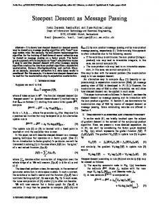
We start by introducing the notion of a solution cluster. We denote by S(F ) the set of satisfying assignments of a CNF formula F . A solution graph for F is an undirected graph, where nodes correspond to solutions and are neighbors if they differ on the assignment of exactly one variable. In other words, the assignments σ, τ ∈ S(F ) are adjacent if they have the Hamming distance equal to 1. A cluster is then a connected component of S(F ). Figure 5.1 illustrates how the structure of the solution space of random 3-SAT evolves as the density of a random formula increases. We summarize the physicists hypothesis of the solution space of random SAT through the following conjectures. 1. There exists a SAT-UNSAT phase transition in the solution space of these problems. More specifically, for clause-variable ratio greater than its critical value αs , solutions cease to exist.


46

}

SAT EASY-SAT

HARD-SAT

αclust = 3.921

UNSAT

αs = 4.267

α = M/N

Figure 5.1: Diagrammatic representation of the solution space of random 3-SAT with respect to α. Satisfying clusters are represented by gray and the unsatisfying by white.

2. Also there exists another threshold αclust , which divides the SAT region into two separate regions, called EASY-SAT and HARD-SAT. In the EASY-SAT region, solutions are thought to be close together such that one can reach from one solution to another with a number of single-bit flips. More specifically, each pair of satisfying assignments are close together in Hamming distance. In this region, local search algorithms and other simple heuristics can easily find a solution. In the HARD-SAT region, the solution space breaks up into many smaller clusters. Each cluster contains a set of satisfying assignments close together in Hamming distance. Also, the satisfying assignments in different clusters are far apart i.e. one cannot reach from a satisfying assignment in one cluster to the one in another without changing a large number of variables. 3. In the HARD-SAT region, there exists an exponentially large number of metastable clusters, i.e. clusters containing almost satisfying assignments (the assignments which violate a few clauses). Also, these almost satisfying solutions violate exactly the same number of clauses. The number of solution clusters are exponential in number of variables N , and the number of metastable clusters too are exponential in N but have a larger growth rate. This suggests that the simpler algorithms like BP get trapped within these most numerous metastable clusters. Moreover, most of the variables in a cluster are frozen, i.e., they take the same value in all the satisfying assignments of the cluster. To describe the Survey Propagation algorithm, which is known empirically to find solutions in the HARD-SAT region, we explain further in detail in the next section, the physical picture of the clustering of configurations.


5.3

47

Solutions Clusters and Covers

Let γ be a cluster in the solution space of a CNF formula F . We denote by S(γ), the satisfying assignments in γ. A variable x can be thought of being in 3 possible states, either (i) it is frozen to 0, i.e. x = 0 in all σ ∈ S(γ) or (ii) it is frozen to 1 in S(γ), or (iii) it switches between 0 and 1, i.e. it takes both of its values in S(F ). To account for the latter case, we extend the domain of x to include a third state “∗” which is also known as the joker state. The above description attributes to each cluster, a single string in {0, 1, ∗}n . We will call such a string over an extended variable space {0, 1, ∗}, as a generalized assignment. In a generalized assignment, a variable can be termed as constrained or unconstrained by the following definition. Definition 5.1. Given a string y ∈ {0, 1, ∗}n , we will say that variable yi is free or unconstrained in y if in every clause c containing yi or ¬yi , at least one of the other literals in c is assigned true or ∗. A variable is constrained if it uniquely satisfies some clause c , i.e. all other literals in c are assigned false. A generalized assignment σ ˆ ∈ {0, 1, ∗}n is called a cover [18] of F if 1. every clause of F has one satisfying literal or at least two ∗, and 2. every unconstrained variable in σ is assigned ∗. Informally, a generalized assignment σ ˆ is a cover if under σ ˆ , either each clause in F is satisfied or it leaves enough variables undecided, which can be set later on to generate a satisfying truth assignment. It is interesting to note that each satisfying assignment in F can be reduced to a unique cover by the coarsening procedure [16] as follows. 1. Given a satisfying assignment, σ, change one of its unconstrained variable to ∗. 2. Repeat until there are no unconstrained variables. To understand the above procedure, consider the formula F = (x ∨ ¬y) ∧ (y ∨ ¬z) and its satisfying assignment (000). Now, x is the only unconstrained variable under this assignment. Setting x to ∗ gives us the generalized assignment (∗00). Now under this new assignment, y is not constrained as it is no longer the unique satisfying literal for any clause. We thus obtain (∗ ∗ 0). The variable z ceases to be the unique satisfying literal for the second clause because of the previous step. We can now change it to ∗. The resulting generalized assignment is now (∗ ∗ ∗) which cannot be further reduced. This corresponds to a cover of the formula F .


48

It is now easy to see that all assignments within a cluster will correspond to a unique cover, also known as core [16] of the cluster.

5.4

The SP Algorithm

SP is a powerful technique for solving satisfiability problems, derived from the rather complex physics methods, notably the cavity method developed for the study of spin glasses. We refer to [19] for the original derivation of the SP equations by the replica symmetric method in statistical physics. Here, we will describe the SP algorithm and show that for tree-structured formulas, SP computes marginals over covers of the formula. We start by describing the notations required for the SP algorithm. The basic input to the SP algorithm is a factor graph for a SAT (random) instance. For each variable node i in the factor graph, we denote the set of factor nodes in which the variable appears positively by N+ (i), and by N− (i) the set consisting of factor nodes in which i appears negated. Here N (i) = N+ (i) ∪ N− (i). Let Nas (i) be the set of neighbors of i except a which tend to satisfy a, i.e., i occurs with the same polarity in any b ∈ Nas (i) as in a. Also Nau (i) represents the set of neighbors which are unsatisfying with respect to a. SP like BP works by passing messages along the edges of the factor graph. A message

N+ (i)

{

i

}

N− (i)

Figure 5.2: A part of a factor graph showing variable node i and its neighboring factor nodes.

from a factor node a to variable node i, known as a survey, is a real number ηa→i ∈ [0, 1]. Each variable i can be in either of the three states in {0, 1, ∗}. A variable takes value 0 or 1 if it is constrained by a clause, i.e., if it satisfies uniquely at least one of the clauses and a joker state otherwise. Each variable node i sends a vector of three real numbers, Πi→a = {Πui→a , Πsi→a , Π∗i→a } to each of its neighboring factor node a. The survey ηa→i


49

over edge {a, i} is given by Y

ηa→i =

j∈N (a)\i

Πuj→a . Πuj→a + Πsj→a + Π∗j→a

(5.1)

The survey ηa→i is interpreted as a probability that a warning is sent from a factor node a to a variable node i [14]. A warning from a factor node a to a variable node i can be understood as a signal that a requires i to take a value that satisfies a which is due to the fact that all variables in N (a) \ i have been assigned values that unsatisfy a. The variable node i sends a message to factor node a corresponding to each of the three symbols {u, s, ∗}. The symbol “s” corresponds to its state which is satisfying for a, “u” stands for the state unsatisfying for a. It sends the symbol “∗” when it is in the undecided or joker state. The corresponding SP equations are Y

Πui→a =

(1 − ηβ→i ) 1 −

β∈Nas (i)

Πsi→a

Y

=

(1 − ηβ→i ) 1 −

β∈Nau (i)

Y

Π∗i→a =

Y

(1 − ηβ→i ) ,

(5.2)

β∈Nau (i)

Y

(1 − ηβ→i ) ,

(5.3)

β∈Nas (i)

(1 − ηβ→i ).

(5.4)

β∈N (i)\a

We will now derive the SP equations for tree-structured factor graphs. The justification for general graphs with cycles suffer from the similar problem as in BP, i.e, the incoming messages to a node can not be considered as independent. The remarkable performance of SP on hard SAT problems suggests the weak correlation among the input messages (to a node). The underlying reason for the same is still unknown.

5.4.1

Deriving SP Equations for Trees

Message Passing algorithms on trees can be thought of as dynamic programming solutions, where a node combines the results (messages) from the neighboring sub-parts of the problem and pass on to the next neighbor which repeats the process. In this section, we show that the messages in BP (for tree-structured SAT formulas) can be interpreted as combinatorial objects counting the number of solutions for some sub-part of the problem. We further show how this counting procedure can be extended to counting covers for the CNF formula. We then prove that the modified message update rules correspond to the SP update equations. In the last paragraph, we claimed that a BP message counts the number of solutions for some sub-part of the problem i.e for some sub-formula of the original formula. To


50

Tj

j

TA

A

D

i

B

C

Figure 5.3: A part of tree-factor graph for a SAT formula.

understand this, consider a variable j in a formula F and suppose that it wants to send the message to its neighboring factor node a about its value xj . We construct a subformula f as follows. We pick variable j and all clauses in which j participates except the clause a. We further include the variables participating in the included clauses and so on. Now the message sent from j to a is the number of solutions of f in which j assumes the value xj . To understand a clause to variable message, we assume that the factor node a has only two neighbors. Now suppose that the node a wants to send a message to its other neighbor i about its value xi . We extend the sub-formula f to include the clause a and the variable i. The message that the factor node a sends to i counts the number of solutions (with i assuming the value xi ) for the extended sub-formula. For SP, we will derive the corresponding message rules according to which a message counts the number of covers instead of solutions. The new beliefs will then correspond to the cover marginals instead of solution marginals. We will now formally present the derivation of the SP equations from BP message update rules. We start by introducing some notations. We consider the tree factor


51

graph T = (V, E) corresponding to a SAT formula F . Figure 5.3 shows a part of T with variable node i and its four neighboring factor nodes. We denote by I(T ) and A(T ), the set of variable and factor nodes (each representing a clause) respectively in T . Recall that the dashed edge between node i and B signifies that the variable i is negated in the clause corresponding to factor node B. Variable to clause messages. Consider the message from variable node j to factor node A. We denote the part of factor graph rooted at j and separated from rest of graph by A (shown in Figure 5.3) by Tj . Also XTj = {xi : i ∈ I(Tj )} represents a configuration of variables in Tj . Y

mj→A (xj ) =

a∈N (j)\A

=

X

ma→j (xj ) Y

(5.5)

fa (Xa ),

(5.6)

XTj \xj a∈A(Tj )

Note that the product term corresponding to each configuration XTj will be 1 if all the clauses in Tj are satisfied and 0 otherwise. The sum operation will in turn count the number of the non-zero terms of the product. Let S(Tj ) denotes the set of satisfying assignments in Tj in which j assumes the fixed value xj . Then the variable to clause message mj→A (xj ) determines |S(Tj )|. We now modify the problem of counting satisfying assignments into that of counting the covers. Let xsa,j /xua,j denote the satisfying/unsatisfying value of j with respect to a, for example, xsA,i = 1 (with respect to Figure 5.3). Also a variable is assigned “∗” if it is not constrained by any of the clauses. We now define our new message, Mj→A (xj ) such that it counts the covers of Tj , in which j assumes the value xj . Consider the message Mj→A (xsA,j ). This message is supposed to count the covers in Tj such that j assumes the value xsA,j under the corresponding generalized assignment, say σg . This further implies that there exists at least one clause c ∈ NAu (j) such that j is the unique satisfying variable for c under σg . Additionally, it is unconstrained by all clauses in NAu (j).

Y

Mj→A (xsj,A ) =

Ma→j (xsj,A ) + Ma→j (∗) −

a∈N (j)\A

Y

=

Ma→j (xsj,a ) + Ma→j (∗)

s (j) a∈NA

−

Y

s (j) a∈NA

Ma→j (∗)

Y

Y

Ma→j (∗)

a∈N (j)\A

Y

Ma→j (xuj,a ) + Ma→j (∗)

u (j) a∈NA

Ma→j (∗)

u (j) a∈NA

(5.7)


52

Similarly, Y

Mj→A (xuj,A ) =

Ma→j (xuj,a ) + Ma→j (∗)

s (j) a∈NA

−

Y

Y

Ma→j (xsj,a ) + Ma→j (∗)

u (j) a∈NA

Y

Ma→j (∗)

s (j) a∈NA

Ma→j (∗).

u (j) a∈NA

(5.8) A node j will assume “∗”, if it is unconstrained in all clauses . Therefore, Y

Mj→A (∗) =

Ma→j (∗)

Y

Ma→j (∗).

(5.9)

u (j) a∈NA

s (j) a∈NA

Clause to variable messages. Now consider the following clause to variable message as in BP mA→i (xi ) =

X

fA (XA )

XA

Y

mj→A (xj ).

(5.10)

j∈N (A)\i

We have seen that the variable to clause message mj→A (xj ) counts the number of satisfying configurations for Tj , with j assuming value xj . Therefore, the product Q j∈N (A)\i mj→A (xj ) counts the number of satisfying assignments in TA for a particular configuration of variables in N (A) \ i. Now, let S(TA ) denote the set of satisfying assignments in TA for all possible values of variables in N (A) \ i . Let variable node i ¯ A ) by including xi such that the clause A is assume value xi . We extend S(TA ) to S(T ¯ A ) . The size of S(T ¯ A ) is precisely the message mA→i (xi ). satisfied in S(T We now give a parallel argument when the product of variable messages

Q

j∈N (A)\i Mj→A (xj )

counts the number of covers of TA . Let C(TA ) denote the set of covers of TA . We ex¯ A ) by including xi such that clause A is satisfied in C(T ¯ A ). Let γ be tend C(TA ) to C(T ¯ A ). We now replace xi in γ by “∗” if clause A has any generalized assignment in C(T been satisfied by variables other than i or there exists at least one more variable in A which has been assigned “∗”. We obtain C¯g (TA ) by repeating the above process for each ¯ A ). The message MA→i (xi ) counts the number of generalized assignments in γ ∈ C(T C¯g (TA ) with i taking value xi . By construction of C¯g (TA ), xi equals xsA,i in some γ ∈ C¯g (TA ) only when each of the variables j ∈ N (A) \ i assumes the value xuA,j , i.e., all variables are unsatisfying except i. Mathematically, this can be stated as MA→i (xsi,A ) =

Y j∈N (A)\i

Mj→A (xuj,A ).

(5.11)


53

Also, there exists no γ ∈ C¯g (TA ) such that xi = xuA,i under γ. Therefore, MA→i (xui,A ) =0.

(5.12)

The message MA→i (∗) will count all the generalized assignments in C¯g (TA ) such that A is either satisfied without i or there exists atleast one other variable which is assigned ∗, i.e., X

MA→i (∗) =

XA \xi

FA (XA )

Y

Mj→A (xj ),

(5.13)

j∈N (A)\i

where   1, if there exists some variable i ∈ N (a) such that xi = xsi,A    Fa (Xa ) = or there exists at least two variables k, l ∈ N (a) with xk = ∗ and xl = ∗ .     0, otherwise (5.14) In other words, MA→i (∗) counts all generalized assignments in C¯g (TA ) except the ones in which each j ∈ N (A) \ i assumes the value xuj,A . We can then write (5.13) as Y

MA→i (∗) =

Mj→A (xsj,A ) + Mj→A (xuj,A ) + Mj→A (∗) −

j∈N (A)\i

Y

Mj→A (xuj,A ).

j∈N (A)\i

(5.15) The message update rules obtained by the extended cover counting procedure are summarized in Figure 5.4. We now derive the beliefs corresponding to the modified message update rules. Beliefs. We consider again the example in Figure 5.3. The belief Bi (xi ) now corresponds to the number of covers of F in which i assumes value xi . We obtain such covers for i by combining appropriate covers from each of TNi . For example, consider Bi (0). We need to count covers of F such that i is constrained to value 0. This means that atleast one clause from N (i) constrains i to 0. Obviously, clauses A and C cannot constrain i to be in the 0 state and, either B or D or both should constrain i to 0. Therefore, Bi (0) =MA→i (∗)MC→i (∗)MB→i (0)MD→i (0) + MA→i (∗)MC→i (∗)MB→i (∗)MD→i (0) + MA→i (∗)MC→i (∗)MB→i (0)MD→i (∗)  Y Y = Ma→i (∗)  Ma→i (xsa,i ) + Ma→i (∗) − a∈N+ (i)

a∈N− (i)

Y

 Ma→i (∗) .

a∈N− (i)

(5.16)


54

Variable to Clause Messages Y

Mi→a (xsa,i ) =

Mb→i (xsb,i ) + Mb→i (∗)

b∈Nas (i)

Y

Y

Mb→i (∗)

b∈Nas (i)

Mi→a (xui,a ) =

Y

Mi→a (∗) =

Mb→j (∗)

b∈Nau (i)

Mb→i (xub,i ) + Mb→i (∗)

b∈Nas (j)

Y

−

Mb→i (xub,i ) + Mb→i (∗)

b∈Nau (i)

Y

−

Y

Y

Mb→i (∗)

b∈Nas (i)

Mb→i (∗)

b∈Nas (i)

Y

Y

Mb→i (xsa,i ) + Mb→j (∗)

b∈Nau (i)

Mb→i (∗)

b∈Nau (i)

Mb→i (∗)

b∈Nau (i)

Clause to Variable Messages Y

Ma→i (xsa,i ) =

Mj→a (xua,j )

j∈N (a)\i

Ma→i (xua,i ) = 0

Y

Ma→i (∗) =

Y

Mj→a (xsa,j ) + Mj→a (xua,j ) + Mj→a (∗) −

j∈N (a)\i

Mj→a (xua,j )

j∈N (a)\i

Figure 5.4: Message update equations for enumerating covers of a formula.

Similarly, we obtain

Bi (1) =

Y

 Ma→i (∗) 

a∈N− (i)

Y

Ma→i (xsa,i ) + Ma→i (∗) −

a∈N+ (i)

Y

 Ma→i (∗) .

a∈N+ (i)

(5.17) Now, i will assume the joker state ∗ in a cover of F , if it is unconstrained in each of the clauses A, B, C, D. Thus, we obtain Bi (∗) =MA→i (∗)MC→i (∗)MB→i (∗)MD→i (∗) Y = Ma→i (∗).

(5.18)

a∈N (i)

We now establish the equivalence of the above described cover counting procedure with the SP update equations for a tree structured SAT formula. Theorem 5.2. Let F be a CNF formula whose factor graph corresponds to a tree. The message update equations (5.4) derived for enumerating covers of F are equivalent to SP update equations for F .


55

Proof. Enforcing the normalization such that Ma→i (xsi,a ) + Ma→i (∗) = 1 we get Y

Ma→i (xsi,a ) =

j∈N (a)\i

Mj→a (xuj,a ) . Mj→a (xsj,a ) + Mj→a (xuj,a ) + Mj→a (∗)

(5.19)

Also, the variable to clause message now becomes Y

Mj→a (xsj,a ) =



0 + Mb→j (∗)

b∈Nau (j)

b∈Nas (j)

−

Y

(1)

Y

Mb→j (∗)



Y

Mb→j (∗)

b∈Nas (j)

 = 1 −

Mb→j (∗)

b∈Nau (j)

b∈Nas (j)

= 1 −

Y

Y

(5.20)

Mb→j (∗)

b∈Nau (j)

Y

 1 − Mb→j (xsj,b ) 

b∈Nas (j)

Y

1−

Mb→j (xsj,b )

.

b∈Nau (j)

Similarly,  Mj→a (xuj,a ) = 1 −

Y



1 − Mb→j (xsj,b ) 

b∈Nau (j)

Y

1 − Mb→j (xsj,b )

(5.21)

b∈Nas (j)

and Mj→a (∗) =

Y

1 − Mb→j (xsj,b ) .

(5.22)

b∈N (j)

Now setting ηa→i = Ma→i (xsi,a ), Πsi→a = Mi→a (xsi,a ), Πui→a = Mi→a (xui,a ) and Π∗i→a = Mi→a (∗) we obtain the following SP equations

Πui→a

Y

Πuj→a , Πuj→a + Πsj→a + Π∗j→a j∈N (a)\i Y Y = (1 − ηb→i ) 1 − (1 − ηb→i ) ,

ηa→i =

b∈Nas (i)

Πsi→a

=

Y

Y

(5.24)

b∈Nau (i)

Y (1 − ηb→i ) 1 − (1 − ηb→i ) ,

b∈Nau (i)

Π∗i→a =

(5.23)

(5.25)

b∈Nas (i)

(1 − ηb→i ).

(5.26)

b∈N (i)\a

We have seen that SP update equations can be used to find the marginals over covers


56

of a formula F if the associated factor graph is a tree. But, these equations can still be applied to general graphs, hoping that they converge and the fixed point beliefs can be used to approximate cover marginals. We now present the SP algorithm for general graphs and then briefly discuss its success in the HARD-SAT region. Algorithm 6 SP Input: A factor graph of a Boolean formula in conjunctive normal form; a maximum number of iterations tmax ; a requested precision Output: Satisfying assignment of the formula (if one exists) 0 1: For t=0, randomly initialize the surveys, ηa→i . 2: Sweep the set of edges in some order and update sequentially the messages on all t edges of the graph, generating a new set of surveys ηa→i , using message update Equations (5.1) (5.2) (5.3) (5.4). 3: for t = 1 to t = tmax do t−1 t 4: if |ηa→i − ηa→i | < for each edge {a, i} then 5: break; 6: end if 7: end for 8: if t = tmax then 9: return UNCONVERGED 10: else ∗ 11: if the fixed point surveys ηa→i are nontrivial i.e.{η 6= 0} then 12: Compute for each variable node i, the biases {Bi+ , Bi− } defined as Bi+ = Bi− =

πi+ + πi− + πi∗

(5.27)

πi− πi+ + πi− + πi∗

(5.28)

πi+

where πi+ πi−

= 1−

Y

Y (1 − ηb→i ) (1 − ηb→i ),

= 1−

b∈N+ (i)

Y

Y (1 − ηb→i ) (1 − ηb→i ),

Y

b∈N− (i)

b∈N+ (i)

πi∗ =

(1 − ηb→i ).

(5.29)

b∈N− (i)

(5.30) (5.31)

b∈N (i)

13:

14: 15: 16: 17:

DECIMATION - Fix the variable with the largest bias, |Bi+ − Bi− | to the value 1 if Bi+ > Bi− , to 0 if Bi+ < Bi− . Reduce the factor graph, by removing the variable and the factor nodes corresponding to the satisfied clauses. If no contradiction is found Go to Step 1, otherwise STOP. else if all the surveys are trivial then Solve the simplified formula by a local search process. end if end if


5.5

57

Discussion

We now discuss the behavior of the SP algorithm with respect to the known empirical results in random SAT problems. The surveys in the SP algorithm may converge at some stage to give a trivial solution, i.e., a {∗}n solution. Such problems may be underconstrained and can be easily solved by other simpler algorithms. The SP can be run again with a different set of initializations, to find a non-trivial fixed point. Numerical experiments show that on large random instances of 3-SAT, in the hard SAT region, but not too close to the satisfiability threshold, the algorithm converges to a non-trivial fixed point. In the other case, the SP algorithm may not converge at some stage, even if the initial problem was satisfiable. This happens in general very close to the satisfiability threshold. It is not yet clear why such a problem arises. The validity of the SP algorithm relies on the conjectures about the phase structure of the solution space of SAT problems. When the solutions organize themselves in well separated clusters, it is believed that the simpler algorithms like BP fail because they get trapped in various local optimal configurations of the sub-parts of the problem. These local optimal solutions can no longer be combined into a global solution. SP is supposed to take into account the clustering phenomena by finding the core of a cluster. Also, it is conjectured that most of the variables inside such cores are frozen, i.e., we have fewer undecided variables. It is then easy to assign the undecided variables by some other simpler method.

Bibliography [1] R. Kindermann and J. Laurie Snell. Markov Random Fields and Their Applications. American Mathematical Society, 1980. [2] S. L. Lauritzen. Graphical Models. Clarendon Press, Oxford, 1996. [3] G. M. Grimmet. A theorem about random fields. Bulletin of London Mathematical Society, 5:81–84, 1973. [4] J. Pearl. Probabilistic Reasoning in Intelligent Systems: Networks of Plausible Inference. Morgan Kaufmann, 1988. [5] J. S. Yedidia, W. T. Freeman, and Y. Weiss. Understanding belief propagation and its generalizations. In Exploring artificial intelligence in the new millennium. Morgan Kaufmann Publishers Inc., 2003. [6] Adnan Darwiche. Conditioning methods for exact and approximate inference in causal networks. In In Proceedings of the 11th Conference on Uncertainty in Artificial Intelligence, pages 99–107. Morgan Kauffman, 1995. [7] Noga Alon, Paul Seymour, and Robin Thomas. A separator theorem for nonplanar graphs. Journal of the American Mathematical Society, 3(4):801–808, 1990. URL http://www.jstor.org/stable/1990903. [8] Y. Weiss. Correctness of local probability propagation in graphical models with loops.

Neural Comput., pages 1–41, 2000.

doi:

http://dx.doi.org/10.1162/

089976600300015880. [9] Yair Weiss and William T. Freeman. Correctness of belief propagation in gaussian graphical models of arbitrary topology. Neural Comput., 13(10):2173–2200, 2001. ISSN 0899-7667. doi: http://dx.doi.org/10.1162/089976601750541769. [10] Thomas M. Cover and Joy A. Thomas. Elements of information theory. WileyInterscience, New York, NY, USA, 1991. ISBN 0-471-06259-6.

58

Bibliography

59

[11] Srinivas M. Aji and Robert J. Mceliece. The generalized distributive law and free energy minimization. In Proceedings of the 39th Allerton Conference, 2001. URL http://www.mceliece.caltech.edu/publications/Allerton01.pdf. [12] Alessandro Pelizzola. Cluster variation method in statistical physics and probabilistic graphical models. J.PHYS.A, 38:R309, 2005. URL doi:10.1088/0305-4470/ 38/33/R01. [13] Marc Mézard and Riccardo Zecchina. Random k-satisfiability problem: From an analytic solution to an efficient algorithm. Phys. Rev. E, 66(5):056126, Nov 2002. doi: 10.1103/PhysRevE.66.056126. [14] A. Braunstein, M. Mézard, and R. Zecchina. Survey propagation: An algorithm for satisfiability. Random Struct. Algorithms, 27(2):201–226, 2005. ISSN 1042-9832. doi: http://dx.doi.org/10.1002/rsa.v27:2. [15] A. Braunstein and R. Zecchina. Survey propagation as local equilibrium equations, 2004. URL doi:10.1088/1742-5468/2004/06/P06007. [16] Elitza Maneva, Elchanan Mossel, and Martin J. Wainwright. A new look at survey propagation and its generalizations. J. ACM, 54(4):17, 2007. ISSN 0004-5411. doi: http://doi.acm.org/10.1145/1255443.1255445. [17] Stephen A. Cook. The complexity of theorem-proving procedures. In STOC ’71: Proceedings of the third annual ACM symposium on Theory of computing, pages 151–158, New York, NY, USA, 1971. ACM. doi: http://doi.acm.org/10.1145/ 800157.805047. [18] Dimitris Achlioptas and Federico Ricci-Tersenghi. On the solution-space geometry of random constraint satisfaction problems. In STOC ’06: Proceedings of the thirtyeighth annual ACM symposium on Theory of computing, pages 130–139. ACM, 2006. ISBN 1-59593-134-1. doi: http://doi.acm.org/10.1145/1132516.1132537. [19] Rémi Monasson and Riccardo Zecchina. Statistical mechanics of the random ksatisfiability model. Phys. Rev. E, 56(2):1357–1370, Aug 1997. doi: 10.1103/ PhysRevE.56.1357.