Method of L-moment estimation for the generalized lambda distribution Paul J. van Staden and M.T. (Theodor) Loots Department of Statistics, University of Pretoria, Pretoria, 0002, SOUTH AFRICA
[email protected]
www.up.ac.za/pauljvanstaden
Abstract The generalized lambda distribution (GLD) is a flexible distribution for statistical modelling, but existing estimation methodologies for the GLD are computationally difficult, rendering the GLD impractical for many practitioners. We derive a parameterization of the GLD with closed-form expressions for the method of L-moment estimators. A numerical example involving the age of coronary heart disease subjects is presented. Keywords: Generalized Pareto distribution, L-moment ratio diagram, quantile function, skew-logistic distribution
properties. Section 5 contains a numerical example and the paper concludes with Section 6.
1. Introduction Although there is no consensus in the literature on the birth date of Tukey’s lambda distribution, with [1] and [2] popular “guesstimates”, the distribution has fathered various offspring, collectively referred to as generalized lambda distributions (GLDs). Among them, two parameterizations have found favour among statisticians and practitioners. Both these parameterizations of the GLD are highly flexible with respect to distributional shape and are hence applied in diverse fields of research. A few recent applications include biochemistry [3], economics [4], forestry [5] and queuing theory [6]. Furthermore, since random variates for Monte Carlo simulation studies can easily be generated via the quantile function (QF) of the GLD, the GLD is often employed in such studies – see for instance [7-9]. Unfortunately, estimating the parameters of the GLD is not straightforward. Various estimation methodologies have been proposed in the literature, but all of them require numerical optimization techniques. We approach the problem from a different angle by not proposing a new estimation method, but by deriving an alternative parameterization of the GLD for which closed-form expressions for the method of L-moment (MoLM) estimators are available. A brief discussion of the theory of L-moments is presented in Section 2. In Section 3 we consider the two parameterizations of the GLD which are currently used in statistical modelling. In Section 4 we derive our parameterization of the GLD and present some of its Third Annual ASEARC Conference
1
2. The Quantile Function (QF) and L-Moments The QF of the probability distribution of a continuous stochastic variable, say X, is defined as Q X ( p) = the value of x such that FX ( x) = p ,
(1)1)
where 0 ≤ p ≤ 1 and FX (x) is the cumulative distribution function of X. The theory of L-moments was compiled by [10]. In terms of the QF, the rth L-moment is defined by 1
Lr = ∫ Q X ( p) Pr*−1 ( p)dp ,
(2)1)
0
where, Pr* ( p) =
r
r r + k k p , k
∑ (−1) r − k k
k =0
(3)1)
is the rth shifted Legendre polynomial. Note that, analogous to [11], we denote the rth L-moment by Lr instead of λr , as is for example done in [10], to avoid confusion with the parameters of the GLD. As proven by December 7—8, 2009, Newcastle, Australia
[10], if the mean of X, µ , exists, then all the L-moments considered the use of shape functionals. Recently [11] exist. L1 = µ is a measure of location, while L2 is a presented MoLM estimation. With all the above-mentioned estimation techniques, measure of spread. L-moment ratios are defined as the four chosen population measures are equated to the corresponding sample statistics, resulting in four L τ r = r , r = 3, 4, ... . (4)1) equations with four unknowns which must be solved L2 simultaneously. Since no closed-form expressions exist for the shape estimators of either the RS or the FMKL The L-skewness ratio, τ 3 , and L-kurtosis ratio, τ 4 , are parameterizations, numerical optimization techniques measures of shape. L-moment ratios are bounded, must be used. The reason is that λ3 and λ4 jointly account for the skewness and the kurtosis of the GLD, simplifying their interpretation. In particular irrespective of the shape measures used. For a detailed 2 1 −1 < τ 3 < 1 and 4 5τ 3 − 1 ≤ τ 4 < 1 . (5)1) discussion on the computational difficulties in fitting the GLD to a data set, the reader is referred to [19].
(
)
Let x1:n ≤ x2:n ≤ ... ≤ xn:n denote an ordered data set of size n. The rth sample L-moment is then given by 4. An Alternative Parameterization for the GLD r −1
r − 1 xir −k :n k
∑ ∑ ... ∑ r −1 ∑ (−1) k
lr =
1≤i1 0
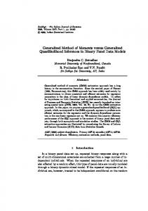
Figure 1. L-moment ratio diagram for the GLD with QF as given in Equation (13).
(−∞ , α ] [α − β λ , α ] (−∞ , ∞ ) [α − (1 − δ ) β λ , α + δ β λ ] [α , ∞ ) [α , α + β λ ]
MoLM estimation is applied to a data set by equating L1 , L2 , τ 3 , τ 4 to l1 , l2 , t3 , t 4 and solving for the unknown parameters in the system of four equations. The advantage of our parameterization over the RS and FMKL parameterizations is that the MoLM estimates can be calculated sequentially using
All L-moments exist for λ > −1 , and are given by L1 = α −
L2 =
β (1 − 2δ ) , λ +1 β
(λ + 1)(λ + 2)
,
(14)1)
(15)1)
r −2
β (1 − 2δ ) s ∏ (λ − i) Lr =
i =1
r
, r = 3, 4, ... ,
(16)1)
∏ (λ + i )
3 + 7t4 ± t 42 + 98t 4 + 1 , 2(1 − t 4 )
(
where s = 1 for r odd and s = 0 for r even. The Lskewness and L-kurtosis ratios are given by (λ − 1)(1 − 2δ ) (λ − 1)(λ − 2) and τ 4 = , (17)1) λ +3 (λ + 3)(λ + 4)
and represented graphically in the L-moment ratio diagram in Figure 1. As with the RS and FMKL parameterizations of the GLD, there is not always a oneto-one relation between the parameter values and the Lmoments. In the dark grey region in Figure 1, two distinct pairs of values for δ and λ give the same pair of L-skewness and L-kurtosis ratios, while a one-to-one relation exists in the light grey regions. It follows from Equation (17) that, irrespective of the value of λ , if δ = 12 , then τ 3 = 0 and the GLD is
(18)1)
)
t λˆ + 3 12 1 − 3 , λ ≠ 1, ˆ λˆ − 1 δ = 1 , λ = 1, 2
(19)1)
( )(
(20)1)
)
βˆ = l2 λˆ + 1 λˆ + 2 ,
i =1
τ3 =
λˆ =
αˆ = l1 +
(
)
βˆ 1 − 2δˆ . λˆ + 1
(21)1)
5. A Numerical Example The coronary heart disease (CHD) data set in [22] contains the age in years of 100 subjects, assumed to have a LOG distribution in a logistic regression framework. A histogram of the data is given by Figure 2 and suggests that the data is approximately symmetric, but that it has tails shorter than the LOG distribution. These visual deductions are confirmed by the sample Lmoments, given in Table 2. Note that, since λ = 0 for the LOG distribution, τ 4 = 16 = 0.1667 from Equation
(17), whereas t 4 = 0.0305 for the data. The generalized secant hyperbolic (GSH) distribution the value of λ , as does all τ 2 r for r ≥ 2 . The minimum and a short-tailed symmetric (STS) distribution were fitted to the data by [23] and [24] respectively. We fitted value of τ 4 is obtained for λ = 6 − 1 .
symmetrical. The L-kurtosis ratio, τ 4 , only depends on
Third Annual ASEARC Conference
3
December 7—8, 2009, Newcastle, Australia
our parameterization of the GLD to the data set. Since (t3 , t 4 ) lies in the dark grey region of Figure 1, we obtained two GLDs, denoted GLD1 and GLD2. Table 2 presents their MoLM parameter estimates, while their density curves are plotted in Figure 2. Both fitted GLDs have bounded support, agreeing well with the data set. Table 2. Sample L-moments and MoLM estimates of the fitted GLDs for the age (in years) of 100 CHD subjects. l1
l2
t3
t4
44.380
6.777
-0.00224
0.0305
αˆ
βˆ
δˆ
λˆ
GLD1
44.768
28.964
0.489
0.627
GLD2
44.140
117.177
0.504
2.688
L-moments
MoLM estimates
Figure 2. Histogram of the age (in years) of 100 CHD subjects with fitted density curves overlayed.
6. Conclusion Using the GPD as a building block, we have derived a parameterization of the GLD which can be easily fitted to a data set using MoLM estimation. In future research we will be focusing on statistical inference for this new member of the Tukey lambda family.
References [1] C. Hastings Jr., F. Mosteller, J.W. Tukey, C.P. Winsor, “Low moments for small samples: a comparative study of order statistics”, The Annals of Mathematical Statistics, 18 (3), 413–426, 1947. [2] J.W. Tukey, “The practical relationship between the common transformations of percentages of counts and of amounts”, Technical Report 36, Statistical Techniques Research Group, Princeton University, 1960. [3] A. Ramos-Fernández, A. Paradela, R. Navajas, J.P. Albar, “Generalized method for probability-based peptide and protein identification from tandem mass spectrometry data and sequence database searching”, Molecular & Cellular Proteomics, 7 (9), 1748–1754, 2008. [4] H.N. Haridas, N.U. Nair, K.R.M. Nair, “Modelling income using the generalised lambda distribution”, Journal of Income Distribution, 17 (2), 37–51, 2008. [5] M. Ivković, P. Rozenberg, “A method for describing and modelling of within-ring wood density distribution in clones of three coniferous species”, Annals of Forest Science, 61 (8), 759–769, 2004. [6] L.W. Robinson, R.R Chen, “Scheduling doctors’ appointments: optimal and empirically-based heuristic policies”, IIE Transactions, 35 (3), 295–307, 2003. [7] F. Bautista, E. Gómez, “Una exploración de robustez de tres pruebas: dos de permutación y la de Mann-Whitney”, Revista Colombiana de Estadística, 30 (2), 177–185, 2007. [8] R. Cao, G. Lugosi, “Goodness-of-fit tests based on the kernel density estimator”, Scandinavian Journal of Statistics, 32 (4), 599–616, 2005. [9] O. Thas, J.C.W. Rayner, D.J. Best, “Tests for symmetry based on the one-sample Wilcoxon signed rank statistic”, Communications in Statistics: Simulation and Computation, 34 (4), 957–973, 2005.
Third Annual ASEARC Conference
4
[10] J.R.M. Hosking, “L-moments: analysis and estimation of distributions using linear combinations of order statistics”, Journal of the Royal Statistical Society: Series B (Methodological), 52 (1), 105–124, 1990. [11] J. Karvanen, A. Nuutinen, “Characterizing the generalized lambda distribution by L-moments”, Computational Statistics & Data Analysis, 52 (4), 1971–1983, 2008. [12] J.S. Ramberg, B.W. Schmeiser, “An approximate method for generating symmetric random variables”, Communications of the Association for Computing Machinery, 15 (11), 987–990, 1972. [13] J.S. Ramberg, B.W. Schmeiser, “An approximate method for generating asymmetric random variables”, Communications of the Association for Computing Machinery, 17 (2), 78–82, 1974. [14] Z.A. Karian, E.J. Dudewicz, Fitting Statistical Distributions: The Generalized Lambda Distribution and Generalized Bootstrap Methods. Chapman and Hall / CRC Press, Boca Raton, Florida, 2000. [15] M. Freimer, G.S. Mudholkar, G. Kollia, C.T. Lin, “A study of the generalized Tukey lambda family”, Communications in Statistics: Theory and Methods, 17 (10), 3547–3567, 1988. [16] J.S. Ramberg, P.R. Tadikamalla, E.J. Dudewicz, E.F. Mykytka, “A probability distribution and its uses in fitting data”, Technometrics, 21 (2), 201–214, 1979. [17] Z.A. Karian, E.J. Dudewicz, “Fitting the generalized lambda distribution to data: a method based on percentiles”, Communications in Statistics: Simulation and Computation, 28 (3), 793–819, 1999. [18] R. King, H. MacGillivray, “Fitting the generalized lambda distribution with location and scale-free shape functionals”, American Journal of Mathematical and Management Sciences, 27 (3–4), 441–460, 2007. [19] Z.A. Karian, E.J. Dudewicz, “Computational issues in fitting statistical distributions to data”, American Journal of Mathematical and Management Sciences, 27 (3–4), 319-349, 2007. [20] J.R.M. Hosking, J.R. Wallis, “Parameter and quantile estimation for the generalized Pareto distribution”, Technometrics, 29 (3), 339–349, 1987. [21] W. Gilchrist, Statistical Modelling with Quantile Functions, Chapman and Hall / CRC Press, Bocca Raton, Florida, 2000. [22] D.W. Hosmer, S. Lemeshow, Applied Logistic Regression, 2nd edition, John Wiley & Sons, Inc., New York, 2000. [23] D.C. Vaughan, “The generalized secant hyperbolic distribution and its properties”, Communications in Statistics: Theory and Methods, 31 (2), 219–238, 2002. [24] A.D. Akkaya, M.L. Tiku, “Short-tailed distributions and inliers”, Test, 17 (2), 282–296, 2008.
December 7—8, 2009, Newcastle, Australia