International Conference on Mathematics, Computational Methods & Reactor Physics (M&C 2009) Saratoga Springs, New York, May 3-7, 2009, on CD-ROM, American Nuclear Society, LaGrange Park, IL (2009)
METHOD OF LONG CHARACTERISTICS APPLIED IN SPACE AND TIME Tara Pandya and Dr. Marvin Adams Department of Nuclear Engineering Texas A&M University College Station, TX 77843-3133
[email protected] [email protected]
ABSTRACT We have developed a long-characteristic (LC) discretization of the time and space variables in the transport equation and tested it in slab geometry. The method’s sole approximation is in the spatial shape of the scattering-plus-fission source. Many LC spatial discretizations assume constant sources in each cell, but because we are interested in thick diffusive problems we must construct sources with at least linear variation in each cell. We have developed a least-squares procedure for constructing such sources. We recognize that it is not possible to simultaneously obtain all three of the following desirable properties: 1) exact solution along each ray in the purely-absorbing limit; 2) cellwise particle conservation; 3) smoothly varying cellwise reaction rates in smooth problems. To illustrate this we construct and display a cellwise-linear scalar flux that produces conservative reaction rates and one that produces smooth reaction rates. These quantities are similar for most cases and the difference between them vanishes in the limit of fine ray spacing. We compare our LC results against results from a traditional linear discontinuous spatial discretization with standard finite-difference time discretizations. We find that our method is more accurate for both streaming-dominated and scattering-dominated test problems. Finally, we remark that application of this method in parallel looks promising, partly due to the independence of the separate rays along which the solution is computed. Key Words: long characteristics, deterministic methods
1. INTRODUCTION We explore the potential benefits of applying the method of long characteristics (MOC) to discretize both spatial and temporal variables in transport problems. We will refer to this long characteristic method in space and time as the space-time long characteristic (STLC) method. Because the streaming plus collision operator (which includes time and space derivatives) is inverted analytically, the only approximation in the method is in the construction of cell-based quantities (reaction rates, scattering sources) from angular fluxes calculated along a finite set of characteristic rays. We introduce a least-squares procedure to construct cell-based quantities that yield smooth cell-to-cell variations in problems with smooth solutions but are not strictly conservative. We also construct “conservative” quantities that yield reaction rates that satisfy the conservation equation in each cell and contrast them with the least-squares quantities. In the limit of fine track spacing the two become the same. The long characteristics method has been applied many times to problems involving multiple dimensions but mostly in steady-state or eigenvalue problems[1][2][3][4]. Here we apply the
Tara Pandya and Dr. Marvin Adams
method to time-dependent slab-geometry transport, in which particle trajectories can be viewed as straight lines in a two-dimensional (x, t) domain. We find that this (x, t) problem presents challenges that are not present in an (x, y) problem, and we discuss how we have addressed these challenges. We employ a linear approximation (in x and t) for the scattering and fission source in each space-time cell, as opposed to the constant approximation found in most MOC implementations [1]. This introduces complexity but also adds significant accuracy, especially in optically thick cells with significant scattering. As previous MOC researchers have found, we find that we are unable to obtain all of the properties that we would like to see in a MOC implementation [1]. These are: * Cell-wise particle conservation; * Exact solution along each ray – no artificial changes in the segments lengths. * Smooth cell-to-cell variation in reaction rates for problems in which the correct reaction rates are smoothly varying. We have implemented a version that gives up cell-wise conservation and another that gives up smooth variations in reaction rates. In both versions, the least-squares fit exactly reproduces the analytic solution in problems for which the analytic solution is linear in x and t, as we demonstrate, and every angular flux along a ray is pointwise exact. Importantly, we show that the conservative method, which produces locally non-smooth reaction rates, does not propagate unphysical information to downstream cells. In fact, somewhat counter to intuition, the conservative method uses a smooth least-squares construction for its scattering source. In the following sections we describe the basic methodology of our STLC method including the relation between coordinate systems and achieving particle conservation. We then present numerical results that demonstrate several key features of the method along with a comparison to traditional methods. We also compare the least-squares and conservative solutions. Finally we conclude with findings and recommendations for uses of this method and further research on this topic. 2. METHODOLOGY In this section we discuss the relation between the x-vt cells defining our problem and the rotated coordinate system defined by particle tracks through our cells. We also derive our least-squares method used to construct the scalar flux function in each cell. We show how this method employs conservative scalar flux values to find the least-squares scalar flux in each cell. 2.1. Coordinate System Definition The purpose of this method is to solve time-dependent slab-geometry transport using long characteristics that span space and time, as an initial exploration toward a similar space-time method for multi-dimensional problems. The spatial and time domains, with coordinates x and t, are discretized into cells with the (i, n)th cell shown in Figure 1. We refer to a characteristic that spans the whole problem as a ray, and the part of the ray in one cell as a track. Figure 1 also shows the tracks for a particular angular direction that pass through this cell.
2009 International Conference on Mathematics, Computational Methods & Reactor Physics (M&C 2009), Saratoga Springs, NY, 2009
2/18
Long Characteristics in Space and Time
tn+1/2
tn
tn-1/2 xi
xi-1/2
xi+1/2
Figure 1: Space-time cell with tracks for one direction
If the vertical axis in Fig. 1 were the spatial variable y, then the distance along each ray would have length units, as would the spacing between tracks. Further, the actual distance traveled by a particle would be the distance shown in the x-y plane divided by the sine of the angle between the trajectory and the plane. In our space-time cell, neither the dotted line segments nor the spacing between them has length units. We can fix this by using vt as our vertical coordinate. However, the actual distance traveled by a particle in our case is simply the change in its vt coordinate – the change in the x coordinate is irrelevant. If one’s intuition was informed by looking at tracks through spatial domains, it can take time to understand the tracks through the space-time domain. We quickly review the solution along a track. If a particle at position x0 at time t0 is moving with direction cosine µ, then after a distance s its x and t coordinates are: x = x0 + µ s t = t0 +
(1)
s v
where v is the particle speed. The analytic transport solution along a characteristic track is:
τ
Ψ m ( x, t ) = Ψ m ( x − µmτ , t − )e v
−σ tτ
τ
s + ∫ dsqtot ,m ( x − µ m s, t − )e−σ t s v 0
(2)
Here τ is distance traveled along the characteristic from (x–µmτ, t–τ/v) to (x, t), and qtot is the total source including scattering (and fission if present). We will need to perform integrals over space-time cells using track spacing and solutions along tracks. We will also need to calculate starting x-t coordinates for tracks that are spaced as 2009 International Conference on Mathematics, Computational Methods & Reactor Physics (M&C 2009), Saratoga Springs, NY, 2009
3/18
Tara Pandya and Dr. Marvin Adams
requested by input. For both of these issues it helps to define a rotated coordinate system in the x-vt plane, as shown in Figure 2. In this figure, θ is related to µ by sinθ = 1/(1+µ2)1/2. Using the relationship in Eq. 1 and the geometric relationships shown in Figure 2, we can relate actual distance traveled (∆s) to distance along the newly defined u axis: ∆u = ∆s / sin θ = ∆s µ 2 + 1 .
(3)
The relation between integrals over (x, vt) and integrals over (ω, u) can be deduced from Figure 2:
∫∫ dxd ( vt ) f ( x, t ) = ∫∫ area
d ω du J f = 1 + µ 2
same area
∫∫
d ω ds f
(4)
same area
(We have used the fact that |Jacobian|=sin2θ +cos2θ=1.) Equation 4 is our guide to approximating integrals over space-time cells in terms of track spacing and integrals along tracks. For example:
∫ dx ∫ d (vt )Ψ m ( x, t ) ≈ ∆x
∆t
# of tracks
∑ k =1
∆ωk 1 + µm2 ∫ dsΨ m ( xk + µm s, tk + s / v). v ∆sk
(5)
In general the area represented by the sum over tracks in Eq. (5) will not exactly equal the actual area v∆t∆x: # tracks
∑
∆ωk ∆sk 1 + µm2 ≠ v∆t ∆x .
(6)
k =1
As track spacing is refined, equality is approached, but this lack of equality for finite track spacing is the source of our inability to achieve all of the desired properties listed previously for the method.
2009 International Conference on Mathematics, Computational Methods & Reactor Physics (M&C 2009), Saratoga Springs, NY, 2009
4/18
Long Characteristics in Space and Time
vt u
δx=∆ω/sinθ
ω v∆t=∆usinθ
θ
vδt=∆ω/cosθ
x ∆x=∆ucosθ
Figure 2: Rotated (w-u) coordinate system in x-vt plane
2.2. Conservation of Particles Next we turn to the construction of the scalar flux function that yields conservation of particles, and in particular that yields conservative reaction rates. The characteristic solution of Eq. (2) satisfies the following conservation equation along the kth track: in Ψ out m , k − Ψ m , k + σ t ∆ sk Ψ m , k =
1 ∆sk σ sφSS ,k + Qkavg . 2
(7)
Here the SS subscript on the scalar flux indicates the scalar flux function that is used in the scattering source, and an over-bar denotes an average (only over track k, not over the cell, in this equation). If we multiply this equation by the track width, ωk, and by (1+µ2)1/2, and divide by speed, then the “in” and “out” terms are the numbers of particles that flow in and out of the space-time cell along the track. If we then sum over all tracks for all quadrature directions we obtain the STLC’s statement of conservation for the cell:
∑ wm ∑ m
k
∆ω k v
in µ m2 + 1 Ψ out m , k − Ψ m , k + σ t ∆s k Ψ m , k −
σ s ∆s k 2
φSS ,k +
∆s k Qk = 0 . 2
(8)
In the limit of fine track spacing, the collision terms become integrals of collision rate density over the space-time cell (see Eq. 5). The five terms in this equation are the numbers of particles 2009 International Conference on Mathematics, Computational Methods & Reactor Physics (M&C 2009), Saratoga Springs, NY, 2009
5/18
Tara Pandya and Dr. Marvin Adams
that: stream into, stream out of, have collisions in, scatter in, and are emitted by the fixed source in the space-time cell. In a conservative method, the scattering term must be σs/σt times the collision term, which implies:
∑ wm ∑ ∆ωk m
µm2 + 1∆sk Ψ m,k = ∑ wm ∑ ∆ωk µm2 + 1
k
m
k
∆sk φSS ,k . 2
(9)
Further, conservation requires that the cell-averaged scalar flux multiplied by v∆t∆x be consistent with this equation; that is,
Φicons ,n ∆tn ∆xi = ∑ wm ∑ m
k
∆ωk v
µm2 + 1∆sk Ψ m,k .
(10)
Here the overbar and the i,n subscript denote an average over the space-time cell. Similar manipulations lead to expressions for the conservative x and t moments of the scalar flux: Φ ix,,ncons ∆xi ∆tn = ∑ wm ∑ m
Φ ti ,,ncons ∆xi ∆tn
k
∆ω k x ∆sk µ 2 + 1Ψ m ,k v
∆ω k = ∑ wm ∑ ∆sk µ 2 + 1Ψ tm,k v m k
(11).
These expressions, however, do not tell us what we should use for the function φSS that is used in the scattering source. If we were assuming constant flux in each cell this would not be an issue; φSS would simply be the conservative average of Eq. (10). In our method, however, the scattering source in a space-time cell is a linear function of x and t, which means n x ,n φiSS , n ( x, t ) = φi + φi
2 ( x − xi ) ∆xi
+ φit ,n
2 ( t − tn ) ∆t n
(12) .
We must find the three φ coefficients that will cause Eq. (9), and similar equations for the x and t moments, to be satisfied. Intuition might suggest that the conservative values given in Eqs. (10) and (11) would be exactly the coefficients needed. If so, intuition would be incorrect! The needed coefficients are those that satisfy the following:
∑ wm ∑ ∆ωk m
k
∑ wm ∑ ∆ωk m
k
∆ sk
1 + µ m2
∫ 0
1 ds Ψ m ( s ) − φiSS , n ( x ( s ), t ( s ) ) = 0 2
(13)
∆ sk
1 + µ m2
1 SS ∫ ds [ x(s) − xi ] Ψ m ( s ) − 2 φi,n ( x(s ), t ( s) ) = 0,
(14)
0
2009 International Conference on Mathematics, Computational Methods & Reactor Physics (M&C 2009), Saratoga Springs, NY, 2009
6/18
Long Characteristics in Space and Time
∑ wm ∑ ∆ωk m
k
∆sk
1 + µ m2
1 SS ∫ ds [t ( s) − tn ] Ψ m ( s ) − 2 φi,n ( x( s), t ( s) ) = 0.
(15)
0
This is equivalent to a least-squares determination of the linear scalar-flux function – minimization of the squared difference between the scalar flux function and the MOC solution when integrated along each track and summed over all tracks for all directions. Recall that the conservative values given in Eqs. (10) and (11) are those that must be used to generate conservative reaction rates in analytic integrals over the space-time cell. However, we see now that these are not the values that should be used in the scattering (or fission) source in the characteristic equation. Instead, to ensure conservation one must use the function given by Eqs. (12)-(15); a function that would not produce conservative reaction rates if analytically integrated over the space-time cell. This is because we need a function that generates the conservative rates when approximately integrated over the cell, with the approximation being the track-based “integration” that appears in many of the equations above. If we use this function in our scattering source, then we obtain a method with the following characteristics: * Cell-wise particle conservation; * Exact solution along each ray – no artificial changes in the segments lengths. * Possibly un-smooth cell-to-cell variation in reaction rates for problems in which the correct reaction rates are smoothly varying; however, these un-smooth rates do not affect the exiting flux from a given cell, because a smooth function is used in the scattering and fission sources in the characteristic equation. Thus, while reaction-rate-based quantities may not be smooth, this does not introduce a lack of smoothness in the angular fluxes calculated by the STLC. That is, the lack of smoothness does not propagate. This is extremely encouraging. So our conservative method does not attain all three desired characteristics, but it misses the third one in a fairly benign way.
3. RESULTS Several simple test problems were used to show the properties of the STLC method and to compare with different LD methods. All of these problems involve one spatial and one temporal variable.
3.1. Test Problem 1: This test problem consists of a multi-cell rectangular grid of uniform width, ∆xi = 0.5 cm, with a solution that is linear in space, angle, and time as shown in Eq. 16. The scattering ratio for this problem is taken to be σs/στ = 0.9 and the cross sections do not vary with position. We vary the track width, ∆ω, from problem to problem. A uniform time step, ∆tn = 0.5 s, is used up to a maximum time of T = 5 s, and a four-point Gauss-Legendre quadrature set is employed. µ (16) ψ ( x, µ , t ) = C0 + C1t + C2 x − σt
2009 International Conference on Mathematics, Computational Methods & Reactor Physics (M&C 2009), Saratoga Springs, NY, 2009
7/18
Tara Pandya and Dr. Marvin Adams
Results demonstrate that the STLC least-squares method exactly reproduces the analytic linear solution for this test problem. Figure 3 shows the non-conservative least-squares scalar flux values for this problem. The solution is the analytic solution to within the iterative convergence tolerance. We find that this result is independent of track width as long as there are at least two tracks that cross each space-time cell. In these and other figures we plot a linear function in each cell, independent of the other cells. The conservative flux values for this problem are also of interest for comparison with the least-squares values and for use in reaction rate calculations. Figures 4 and 5 show the conservative flux values for this test problem with a coarse track spacing of ∆ωk = 0.5 cm and a fine track spacing of ∆ωk = 0.05 cm. As expected these conservative flux values are not quite linear and show the lack of smoothness that we expected. However, despite the extremely coarse ray spacing, which causes the gradient in many cells to be far from the analytic solution’s gradient, the global shape and magnitude is correct. This is because, as we observed above, the functions that affect the exiting fluxes from a cell are smooth functions that know nothing about the erroneous gradients in the conservative function.
120
scalar flux
100 80 60 40 20 0 6 5
4
4 3
2 t
2 0
1 0
x
Figure 3: Non-Conservative (least-squares) Scalar Flux
2009 International Conference on Mathematics, Computational Methods & Reactor Physics (M&C 2009), Saratoga Springs, NY, 2009
8/18
Long Characteristics in Space and Time
120 100 scalar flux
80 60 40 20 0 6 5
4
4 3
2
2 0
t
1 0
x
Figure 4: Conservative Scalar Flux with Coarse Track Spacing (∆ωk = 0.5 cm)
120
scalar flux
100 80 60 40 20 0 6 5
4
4 3
2 t
2 0
1 0
x
Figure 5: Conservative Scalar Flux with Fine Track Spacing (∆ωk = 0.05 cm) 2009 International Conference on Mathematics, Computational Methods & Reactor Physics (M&C 2009), Saratoga Springs, NY, 2009
9/18
Tara Pandya and Dr. Marvin Adams
Note further that as the track spacing is refined, the conservative flux approaches the smooth analytic solution, as shown in Fig. 5.
3.2. Test Problem 2: This second test problem is designed to compare this STLC method to standard methods as applied to a streaming problem. The two methods used for comparison employed the linear discontinuous (LD) method in the spatial variable; one used implicit (backward) Euler in time and the other used Crank-Nicholson. The test problem consists of a multi-cell rectangular grid of uniform cell width. Also the time step was uniform up to a maximum time of T = 1 s. The source of particles consists of an incident beam on the left side of the slab. Therefore the boundary and initial conditions are the following: m ψ inc = ψ 0 , µm > 0, m = 0, ψ inc
µ m < 0,
ψ ( x, 0) = 0, x ∈ (0, L) An S4 quadrature set was used for both STLC and the LD methods. Thus, the problem is basically the superposition of two beam problems, one for each positive µ. The scattering ratio for this problem is taken to be σs/στ = 0.2 with varying track width for STLC defined by ∆ω. It should be noted that the value of the total cross section was very small, on the order of 1E-4, therefore the absorption cross section was also very small. Again a minimum of two tracks per cell were needed in order for the conservative and non-conservative procedures to have sufficient information to build linear functions of x and t. Figure 6 shows the conservative and non-conservative least-squares scalar flux solution to this problem with a cell width of ∆x = 0.05 cm, a time step of ∆t = 0.1 s, and a track spacing of ∆ωk = 0.01 cm. Figure 7 shows the LD scalar flux solution using fully implicit Euler and Crank Nicholson methods. Note that the scalar flux should be zero in part of the space-time domain, constant in the part reached by only one beam (the one with the largest µ), and a larger constant in the remainder of the domain (where both beams have reached). We see that the STLC method clearly defines the expected regions of constant solution for this beam problem, both for the conservative and non-conservative values. The STLC method does not suffer the smearing in time associated with the fully implicit solution shown in Fig. 7(a), nor does it suffer from oscillations like the Crank-Nicolson solution. The conservative STLC solution is smooth in this problem, likely because there are several tracks per cell.
2009 International Conference on Mathematics, Computational Methods & Reactor Physics (M&C 2009), Saratoga Springs, NY, 2009
10/18
Long Characteristics in Space and Time
(a)
(b) Figure 6: (a) Conservative STLC Scalar Flux; (b) Non-Conservative STLC Scalar Flux 2009 International Conference on Mathematics, Computational Methods & Reactor Physics (M&C 2009), Saratoga Springs, NY, 2009
11/18
Tara Pandya and Dr. Marvin Adams
(a)
(b) Figure 7: (a) Fully Implicit LD Solution; (b) Crank-Nicholson LD Solution 2009 International Conference on Mathematics, Computational Methods & Reactor Physics (M&C 2009), Saratoga Springs, NY, 2009
12/18
Long Characteristics in Space and Time
3.3. Test Problem 3: This test problem is designed to compare this STLC method to LD methods as applied to a diffusive problem. Again, implicit Euler and Crank Nicholson were used for the LD methods. This problem is also a multi-cell rectangular grid. The total width of the problem is 10.1 cm with a constant isotropic source in the center of the material. The source and material regions have the following properties:
σs = 1.0 σt m = 0, ψ inc
µ m > 0,
m = 0, ψ inc
µ m < 0,
ψ ( x, 0) = 0, x ∈ (0, L) Source region: q ( x, µ m ) = C ,
x ∈ ( 5,5.1) cm, m = 1,..., M
σs = 1.0 σt ∆xsource = 1 mm Figure 8 shows the setup of this test problem. The time step and cell width, excluding the source regions, were uniform up to a maximum time of T = 2 s. We can find the analytical solution to the diffusion problem which is given in Eq. 17. 1 ∂φ ∂ 2φ x, t ≠ 0 −D 2 =0 v ∂t ∂x φ ( x, 0) = 0, x ≠ 0 (17) φ (0, t ) = S0 , x = 0 The general solution to this problem is given in Eq. 18. x2 exp − 4vDt φ ( x, t ) = C (18) t To find our actual solution we must apply the source condition given in Eq. 19. S δ ( x) , t > 0 S ( x, t ) = 0 (19) t≤0 0, (We have approximated our thin source region as a delta-function plane source.) Therefore the analytical solution to this diffusion problem is given in Eq. 20. t
φ ( x, t ) = S0C ∫ dt ' 0
−
e
x2 4 vD ( t −t ')
t −t'
,
t >0
(20)
Figure 9 shows a plot of the analytic diffusion solution scalar flux ignoring the magnitude of the solution. Solving the associated transport problem with an S2 quadrature, we expect to find 2009 International Conference on Mathematics, Computational Methods & Reactor Physics (M&C 2009), Saratoga Springs, NY, 2009
13/18
Tara Pandya and Dr. Marvin Adams
almost the same results as the solution of the diffusion equation. Some difference may appear, for S2 is equivalent to P1, and P1 differs from diffusion in that it does not ignore the time derivative of the net current density.
q=0 c=1
q=0 c=1 q(x,µ) = C
x=0
x=L
∆x = 1 mm Figure 8: Geometry of Test Problem #3
2.5
3 2.5
2 scalar flux
2 1.5
1.5
1 0.5
1
0 2 0.5
1.5 1
5 0.5
time [s]
0 0
-5
0
x [cm]
Figure 9: Analytic Scalar Flux for plane-source diffusion problem. 2009 International Conference on Mathematics, Computational Methods & Reactor Physics (M&C 2009), Saratoga Springs, NY, 2009
14/18
Long Characteristics in Space and Time
Figure 10 shows the conservative and non-conservative scalar flux values from the STLC code for a cell width of ∆x = 0.25 cm, a time step of ∆t = 0.1 s, and a track spacing of ∆ωk = 0.01 cm. Figure 11 shows the scalar flux solution from the LD code using a fully implicit and Crank Nicholson scheme with the same cell width and time step. Comparing these figures to the analytical solution shown in Fig. 9, we see that the STLC and LD codes all produce the correct flux shape given these relatively fine spatial and temporal grids. However, we can see that the STLC method does not over-diffuse the solution as much as the LD methods. (We remark that early in time, when the solution has high spatial gradients near the source, the spatial grid does not resolve the gradients and the linear STLC functions dip negative in the cells adjacent to the source.) The main conclusion from this test problem is that STLC is accurate for diffusive problems as well as streaming problems.
(a)
2009 International Conference on Mathematics, Computational Methods & Reactor Physics (M&C 2009), Saratoga Springs, NY, 2009
15/18
Tara Pandya and Dr. Marvin Adams
(b) Figure 10: (a) Conservative STLC Scalar Flux; (b) Non-Conservative STLC Scalar Flux
2009 International Conference on Mathematics, Computational Methods & Reactor Physics (M&C 2009), Saratoga Springs, NY, 2009
16/18
Long Characteristics in Space and Time
(a)
(b) Figure 11: (a) Fully Implicit LD Solution; (b) Crank-Nicholson LD Solution 2009 International Conference on Mathematics, Computational Methods & Reactor Physics (M&C 2009), Saratoga Springs, NY, 2009
17/18
Tara Pandya and Dr. Marvin Adams
4. CONCLUSIONS We have developed a long characteristic method in space and time that can accurately find the solution of diffusive and streaming problems. We have designed the method to be exact for problems that have linear solutions in space and time. The method uses a least-squares fit to find non-conservative flux values with the only approximation being in the distribution of the source term. The STLC method can also produce conservative flux values which preserve reaction rates. Although for some problems this conservative method may produce un-smooth reaction rates from cell-to-cell, this lack of smoothness does not propagate or affect the smoothness of the exiting flux from a cell. Therefore we have developed a method that can get very close to the three desired quantities we want: cell-wise particle conservation, the exact solution along a ray, and smooth reaction rates when they should be smooth. There are many further research areas including extending this method to higher dimensions and more realistic problem applications. As mentioned previously, this method could be very useful for radiative transfer, in which some regions can be optically thick and dominated by absorption and re-emission. The method also lends itself to adaptivity in which the track width can be refined for regions requiring finer resolution. Also, extending this method to a parallel scheme is a further research area that could be very interesting. Since the solution along each ray in a problem can be found separately in this method, the division amongst many processors is a logical step. Therefore, the scalability of this STLC method in parallel looks very promising.
ACKNOWLEDGMENTS We thank Jim Morel for many helpful discussions.
REFERENCES 1. M. R. Zika and M. L. Adams, “Transport Synthetic Acceleration for Long-Characteristics Assembly-Level Transport Problems,” Nucl. Sci. Eng. 134, 135, (2000). 2. G.S. Lee, et al., “Acceleration and Parallelization of the Method of Characteristics for Lattice and Whole-Core Heterogeneous Calculations,” Proc. Int. Mtg. Advances in Reactor Physics and Mathematics and Computations into the new Millenium, Pittsburgh, PA, 2000, American Nuclear Society (2000). 3. K. S. Smith and J. D. Rhodes, “CASMO-4 Characteristics Method for Two-Dimensional PWR and BWR Core Calculations,” Trans. Am. Nucl. Soc., 83, 294 (2000). 4. K.S. Smith and J. D. Rhodes, “Full-Core, 2-D, LWR Core Calculations with CASMO-4E,” Proc. Int. Conf. on the New Frontiers of Nuclear Technology: Reactor Physics, Safety and HighPerformance Computing, Seoul, Korea, Oct. 7-10 (2002).
2009 International Conference on Mathematics, Computational Methods & Reactor Physics (M&C 2009), Saratoga Springs, NY, 2009
18/18