Methodologies for Qualitative Spatial and Temporal Reasoning Application Design
Carl Schultz Department of Computer Science, The University of Auckland Private Bag 92019, Auckland, New Zealand Robert Amor Department of Computer Science, The University of Auckland Private Bag 92019, Auckland, New Zealand Hans W. Guesgen School of Engineering and Advanced Technology, Massey University Private Bag 11222, Palmerston North, New Zealand
ABSTRACT Although a wide range of sophisticated qualitative spatial and temporal reasoning (QSTR) formalisms have now been developed, there are relatively few applications that apply these commonsense methods. To address this problem we are developing methodologies that support QSTR application design. We establish a theoretical foundation for QSTR applications that includes the roles of application designers and users. We adapt formal software requirements that allow a designer to specify the customer’s operational requirements and the functional requirements of a QSTR application. We present design patterns for organising the components of QSTR applications, and a methodology for defining high level neighbourhoods that are derived from the system structure. Finally, we develop a methodology for QSTR application validation by defining a complexity metric called H-complexity that is used in test coverage analysis for assessing the quality of unit and integration test sets.
1.0 INTRODUCTION Over the last two and a half decades researchers have made significant progress in the theoretical foundations and analysis of qualitative spatial and temporal reasoning (QSTR) calculi, and a range of commonsense formalisms have now been developed for representing and reasoning about different aspects of space and time (Cohn & Renz, 2008). Moreover, while many QSTR formalisms have been shown to be NP hard, maximal tractable subsets of well known calculi have been identified (Nebel & Bürckert, 1995; Renz, 1999) and automatic methods for finding tractable subsets have been developed (Renz, 2007), thus informing a user about the classes of
problems that are practical to solve. Techniques have also been developed that greatly improve reasoning performance (Westphal & Wölfl, 2009; Li et al., 2009). Despite this theoretically advanced state of the field, there is a distinct absence of applications that make significant use of QSTR formalisms. There are five critical barriers to QSTR application design that have not yet been addressed. 1. QSTR researchers have not clearly identified the characteristics of the problems that can be uniquely addressed by QSTR applications. 2. In many cases, no pre-existing QSTR formalism will perfectly and completely satisfy the requirements of an application. In most cases the designer will need to formalise domain knowledge, and design complex, heterogeneous models that build on top of a mix of different existing QSTR formalisms. 3. There is no methodology for developing QSTR applications, and even researchers in the field currently develop QSTR applications in a very ad hoc manner. 4. There are no methodologies for analysing QSTR applications, and therefore no way to make informed design decisions. This contributes to the problem of ad hoc QSTR application development. 5. Making QSTR accessible means having designers from outside the field applying QSTR, that is, the designers will not be experts in QSTR. Design methodologies derived from concepts in software engineering are required to bridge the gap between expert QSTR logicians and application designers from other disciplines. We address these issues in this chapter with specialised methodologies for QSTR application design, motivated by research in software engineering, knowledge representation, artificial intelligence, and finite model theory. Section 2 reviews unifying frameworks and development tools in related areas and establishes a theoretical foundation for QSTR applications. Section 3 identifies the salient characteristics of QSTR applications that are the focus of our design methodologies. Section 4 characterises the problems that QSTR applications address and enumerates the tasks that they can perform, by adapting formal software requirements from software engineering. Section 5 presents design patterns for organising the components of QSTR applications, and Section 6 presents a methodology for defining high level neighbourhoods that are derived from the system structure. Section 7 presents a methodology that supports designers in QSTR application validation by identifying important classes for unit testing and integration testing based on a novel measure of complexity. Sections 8 and 9 present the future work and conclusions of this chapter.
2.0 BACKGROUND A number of unifying QSTR frameworks are now being developed in order to make the field more cohesive and accessible. Three prominent projects are SparQ (Dylla, 2006), GQR (Gantner, 2008), and an investigation into formal algebraic properties (Ligozat, 2004). Although developing a library of efficient and robust implementations of QSTR calculi is a necessary step in making these formalisms more accessible, this does not directly address the five key problems given in the introduction. Researchers in the related field of qualitative reasoning (QR) have developed a workbench software application called Garp3 (Bredeweg, 2007) to support the process of designing and reasoning with qualitative models. Note that QR is distinct from QSTR as it is primarily concerned with treating scalar quantities in a qualitative discrete way, rather than directly
modelling commonsense spatial and temporal relationships. Garp3 is an integrated development environment for designing and reasoning about qualitative models of physical systems. The motivation for Garp3 is identical to the problems that the QSTR field currently encounters, namely that wider audiences can be reluctant to employ the advanced methods for modelling qualitative physics that have been developed (although this problem does not appear to be as significant as with QSTR, for example (Iwasaki, 1997)). The central aim of Garp3 is to overcome this inertia by supporting modellers in specifying and reasoning about qualitative models in a graphically based, user-friendly, homogeneous workbench. A QSTR equivalent to Garp3 would be highly desirable. In the field of software engineering the well known Unified Modelling Language (UML) is used to specify and visualise object oriented software systems (Pooley, 2004). UML is particularly relevant because it is well known within the software engineering community, and thus by adapting UML concepts (such as use cases and object classes) we can help to bridge the gap between software engineers and QSTR logicians. According to standard software engineering practices, formal software requirements are necessary for software development and validation (Burnstein, 2003). Defining equivalent formal requirements for QSTR applications may also be necessary for the development of powerful QSTR based applications. Five standard requirements categories are operational requirements, functional requirements, performance requirements, design requirements, and allocated requirements (SETC, 1984). In Section 4 we adapt two of these requirements, namely customer’s operational requirements and functional requirements, to the QSTR application domain. We also provide methodologies adapted from UML to support the designer in specifying QSTR application requirements.
2.1 Definition of QSTR Applications Informally, QSTR applications model, infer, and check the consistency of object relations in a scenario. We will define QSTR applications in terms of model theory (Marker, 2002; Hodges, 1997) and then define the roles of QSTR application designers and users. We use the notation ↑ to represent the exponent operator, x↑y=xy. In model theoretic terms, a language L (or vocabulary, or signature) is a finite set of relation symbols R and arities aR for each R∈R. A model M of language L (or L-structure, or interpretation) consists of a universe U (or domain, or underlying set) and for each relation symbol R∈R there is a set RM ⊆ U ↑aR. That is, M provides a concrete interpretation of the symbols in L based on the underlying set U. Finally, a scenario (or configuration, or substructure) is a model V that can be embedded into M, that is, an injective homomorphism f:V→U exists such that, for each R∈R with arity a, a ∀ v1,…,va∈V ⋅ (v1,…,va)∈RV ↔ (f(v1),…,f(va))∈RM.
A QSTR application has a language L that specifies the set of relation symbols that the designer has deemed relevant to the task at hand. The model M of a QSTR application is the interpretation of the relations, implemented using first order constraints between the relations (what objects must, or must not, exist in different combinations of relations). For each relation type R∈R with arity aR, and for each tuple of arity aR, the relation either holds, does not hold, or is not applicable for that tuple. Thus, for each relation symbol R∈R in the language, a QSTR
application model M requires three sets, RM+ (holds), RM− (does not hold) and RM~ (not applicable), with the axiom Axiom 1.
+ ~ ∀ R∈R ⋅ U ↑aR = RM Δ RM− Δ RM ,
where Δ is symmetric difference (the set theoretic equivalent of mutual exclusion). For brevity we will omit the M and simply write R+. A QSTR application designer is responsible for determining the application language and model, given formal software requirements. This involves selecting an appropriate set of relation symbols and encoding an appropriate set of constraints. Appropriateness means satisfying specific test criteria and conditions on metrics that imply that the software requirements have been met. A QSTR application user constructs scenarios in a QSTR application by specifying a model V and employing reasoning to accomplish tasks such as determining scenario consistency with respect to the model M, envisioning potential future scenarios, and so on (a complete set of basic QSTR application task types with respect to this model of QSTR applications is presented in Section 4). Table 1 summarises the relationship between model theory, QSTR applications, and actor roles. Model Theory language L
QSTR Application Domain specification of useful qualitative relations
model M based on L
constraints that determine the interaction between the relations
model V based on L embedded in M
Using a QSTR application to represent and reason about objects.
Actor
QSTR application designer
QSTR application user
Table 1. Comparing the domains of model theory, QSTR applications, and the roles of QSTR application designers and users. Often parts of the user’s scenario are indefinite or unknown, and reasoning with the application constraints is used to help resolve this ambiguity. For each relation R∈R, the user can place tuples (of objects from V) with arity aR in a fourth indefinite set, RM? that is mutually exclusive with the three corresponding definite sets. This partial scenario is a shorthand for specifying a set of models V1,…, Vn each representing a possible scenario. An example of a scenario is V={kitchen, lounge, study}, adjacent+ ={(lounge, study), (lounge, kitchen)}, adjacent? ={(lounge, lounge), (study, lounge), …}, adjacent− ={}, adjacent~ ={}. The adjacent relation can be defined as symmetric using the constraint {(x,y) | (y,x) ∈ adjacent+} ⊂ adjacent+. The LHS of the constraint as evaluated in the scenario is {(study,lounge),
(kitchen,lounge)}. The RHS as evaluated in the scenario does not contain these tuples as required by the proper subset relation, and so reasoning moves the offending tuples out of adjacent? and into adjacent+ thus satisfying symmetry.
2.2 Fundamental Operations on QSTR Scenarios In this section we use our model theoretic definitions to derive the complete set of fundamental operations that can be performed on a QSTR application model. In Section 4 we combine these operations to enumerate a set of basic purely qualitative tasks, and show how the application designer can use this information to determine their software requirements, and to develop their QSTR application. Given a partial scenario, what operations can be performed on the model theoretic structure? The features involved are language symbols, constraints, the scenario universe, and the collection of sets that interpret the relation symbols. The relation symbols and constraints are determined at QSTR application design time and so are fixed when reasoning about scenarios. Once a partial scenario has been specified, either the user has declared all the relevant objects, and thus the set is also fixed, or objects may appear and disappear from the set (e.g. in dynamic scenarios). Thus, the only component that is variable in all scenarios is the set of interpreting models, that is, which models are included and which models are excluded from the partial scenario (although the models themselves are immutable). Furthermore, in some applications the set of objects may also be variable. This leaves only three fundamental operations that can be performed on a qualitative (partial) scenario: • selecting subsets of tuples in the partial scenario, • refining the partial scenario by eliminating particular complete scenarios, and • editing the set of objects in the scenario. Therefore, all QSTR application tasks can be defined as a series of tuple selections, partial scenario refinements and scenario universe edits. Table 2 illustrates a comparison between actor roles, variable components, and permitted operations on QSTR scenarios.
M L application design scenario design scenario reasoning
V’ M
V
V
permitted operations select refine edit tuples scenario objects
V
Rα
R?
v
n/a
n/a
n/a
n/a
c
c
v
v
v
n/a
c c
c c
c v
c c
v v
M
R
v
v
c c c
9 9
9 9
8 9
Table 2. Defines permitted fundamental operations on QSTR scenarios based on the combination of components that are variable. The left hand column assigns actor roles to variables available. Variables are represented by v, constants by c, non-applicable components by n/a, available operations by 9, and unavailable operations by 8. Partial scenario models distinguish between definite relations where α={+,−,~}, and indefinite relations.
3.0 CHARACTERISTICS OF QSTR APPLICATIONS
This section presents four central properties of QSTR applications. We argue that methodologies for the development of QSTR applications must focus on supporting the designer in these four areas.
3.1 Reasoning Across a Broad Range of Abstraction Levels QSTR applications often employ a broad range of abstraction levels in the same model. For example, a QSTR application can model very abstract high-level emotional responses and very low-level concrete spatial configurations of light fixtures, compared to a numerical GIS database that simply stores numerical descriptions of features (points and lines describing a polygon for a region). QSTR application designers require special techniques for rapidly designing and validating models that have a very layered and hierarchical structure. Section 5 presents the concept of fragments and two design patterns for organising QSTR application relations.
3.2 Continuity Assumption And Neighbourhoods For Changing Scenarios QSTR relies heavily on the concept of continuity, stating that temporal and spatial objects cannot morph and translate discontinuously, but must change in a continuous fashion. A fundamental relationship exists between continuity and compositional reasoning (the prominent reasoning mechanism for standard QSTR calculi), and is used directly in critical QSTR tasks such as envisioning. Continuity is formally defined using conceptual neighbours and neighbourhood graphs (Freksa, 1992). The standard definition of conceptual neighbours is (Cohn, 2008), R1 and R2 are conceptual neighbours if it is possible for R1 to hold over a tuple of objects at one point in time, and for R2 to hold over the tuple at a later time, with no other mutually exclusive relation holding over the tuple in between. A neighbourhood graph has one node for each relation R∈R and an edge between two nodes if the corresponding relations are neighbours. Section 6 generalises the definition of conceptual neighbours to apply to QSTR applications, and presents a methodology for designers to customise their conceptual neighbour definitions.
3.3 Modelling Infinite Domains QSTR application models typically have infinite domains, in contrast to, for example, relational database models and constraint satisfaction programming (CSP) models which typically have finite domains (Cohn & Renz, 2008). This significantly complicates the process of validating a specific QSTR calculi's reasoning mechanism so that even expert logicians find this to be a nontrivial task (Wölfl et al., 2007). When considering the perspective of QSTR applications, two further problems are that QSTR applications are significantly more complicated than a given calculi, and the application designers are not necessarily expert logicians. Thus, more practical software engineering based approaches to validating constraints over infinite domains are required for QSTR applications. Section 7 presents novel test coverage metrics for QSTR application validation by adapting complexity measures and techniques from finite model theory.
3.4 Reasoning About Objects in Multi-Dimensional Models QSTR applications very often model multi-dimensional structures. Prominent tasks that use qualitative reasoning, particularly composition, apply transitivity to determine whether a scenario is consistent, and thus rely on relations having an ordering. In QR relations map to scalar one dimensional quantities, and thus have an obvious total order. On the other hand, spatial scenarios
often apply at least two dimensions, thus admitting only partial orderings. Temporal scenarios can also apply multiple dimensions in the form of branching and parallel time streams, resulting in a partial ordering of events. Multi-dimensional models significantly complicate the design of qualitative reasoning methods, as the designer needs to determine the structure of the partial ordering to employ transitivity. This issue is the focus of future research.
4.0 FORMAL SOFTWARE REQUIREMENTS FOR QSTR APPLICATIONS In this section we adapt two standard formal requirements from software engineering, namely customer’s operational requirements and functional requirements, to the QSTR application domain.
4.1 Customer’s Operational Requirements Customer’s operational requirements define the essential needs of the customer (SETC, 1984). In particular, operational requirements specify • the context of deployment, • the typical environment in which the application must function correctly, • how the application will address the current problem (mission profile), • the critical aspects of the application, • how the application will be used, • the application’s minimum allowable efficiency required to solve the problem, and • the operational life cycle. We now define critical characteristics of QSTR problems, and show how these characteristics determine the customer’s operational profile. By considering how each of these characteristics relate to the problem at hand, the designer can formalise the requirements of the application. Figure 1 illustrates an appropriate sequence for considering some of the application characteristics based on their dependencies. The collection of characteristics presented below has been developed from an analysis of the formal definitions of QSTR applications, for example to determine what aspects of a model can vary between applications, such as initial or ongoing dependency, and a review of QSTR literature, for example to determine the different environments for which researchers have developed calculi.
initial
develop
ongoing
query both
Model dependency
Task categories
change
monotonic
stable
non-monotonic
volatile
static
Model lifetime
Model change
Model stability
Figure 1. QSTR problem characteristics, ordered according to the dependencies between characteristics.
Model dependency: the duration of dependency on the working model during the problem solving process. A problem may only have initial dependency, where all the information required for processing is initially available, for example, checking the qualitative consistency of an existing spatial database. Alternatively other problems require information that is not initially available and thus the dependency on the working model is ongoing, for example, checking the consistency of a spatial database whenever modifications are made. Task categories: QSTR tasks fall into two basic categories, either querying the model or developing the model. Further task details are specified in the functional requirements. Model lifetime: the state of the application’s working model over its lifetime. Once initialised the working model may never change, for example, bootstrapping a robot with a qualitative description of an environment on which the robot runs qualitative queries for accomplishing navigation tasks. Alternatively, the working model may change, for example, if a robot performs simultaneous qualitative location and mapping. Model change: models either change monotonically or non-monotonically. Model stability: the frequency of changes that occur to a model. Models are either stable and changes occur rarely, or volatile and changes occur frequently. Element relationships: elements in a model can have simple relationships, with only superficial or limited interaction, for example, a GIS application that describes the qualitative spatial relationships between arbitrary features in terms of orientation and proximity. Alternatively, model elements can have complex relationships, with a lot of significant interaction and strong dependencies, for example, a town planning GIS application that incorporates a high degree of semantic content about the types of buildings being modelled, and constraints between buildings such as ensuring all residences are suitably accessible from some fire station. Spatial Granularity: the spatial context of the application model primarily defined by the scale. Basic categories of environments for which existing QSTR calculi have been designed to reason about, ranging from smallest to largest, are: hand (e.g. inside a pencil case), desktop, indoor, outdoor (e.g. a sports field), neighbourhood, geographical, and astronomical. Spatial Dimensionality: the number of dimensions used to model spatial relationships, typically a combination of one, two, or three dimensions, and may also model arbitrary dimensions. Spatial and Temporal Entities: the context of the application model in terms the entities being modelled. This includes time points, time intervals, spatial points, spatial intervals (directed or undirected), and spatial regions. While this set of characteristics is likely to be incomplete, it establishes a methodology for specifying the customer requirements of a QSTR application. Future research will focus on expanding the list of characteristics, and determining which characteristics are the most significant.
4.2 Functional Requirements Functional requirements define what tasks the system needs to be capable of performing, and how the system will behave during execution (SETC, 1984). These requirements are specified as the inputs, behaviours, and outputs of system components. In this section we enumerate the basic set of purely qualitative tasks that includes tasks commonly found in the QSTR literature. The set of basic QSTR tasks are derived by considering all possible sequences of operations that can be
performed on the application parameters, namely the set of relations, constraints, and the universe. Therefore, this derivation defines the exact extent to which QSTR can be applied, and thus provides a standard with which a software developer can determine, firstly, whether or not QSTR is applicable to their problem, and secondly, what specific qualitative tasks may be suitable for their problem.
4.2.1 Deriving Standard QSTR Tasks Using Fundamental Operations We define a task as a sequence of operations on a mathematical structure. The set of basic QSTR tasks is established by considering sequences of operations that can be performed on the parameters of a scenario in a QSTR application. As presented in Section 2.1, an application has a set of relations R and constraints C. A scenario consists of a universe V and a set of relation state sets R. As presented in Section 2.2, the fundamental operations that can be applied to scenarios are selection, refinement and editing the scenario universe (adding or removing objects). The select operator can only be performed on application parameters, i.e. R, C, and V. During application runtime the only variables are V and the relation state sets. This limits the number of task categories that can be performed, which will now be enumerated. Table 3 presents a summary of the basic tasks and their associated model parameters. The most basic task is to simply execute a selection operation. Querying is used to isolate relevant subsets of a model. For example, in (Qayyum & Cohn 2007) the authors use a qualitative description of images (adapted from Allen’s interval calculus) to provide a method for searching through an image database based on semantic content. TreeSap (Schultz, et al. 2007) is a geographic information system that accepts qualitative queries such as “find all bus stops near Downtown” and displays objects that meet the given criteria. In many cases, a QSTR application user may not have complete information about the criteria of the query that they want to execute, for example, a robot reasoning with noisy sensor readings (Dylla & Wallgrün, 2007). It may be the case that certain conditions are more flexible than others, and moreover, if a user executes a query that returns no results, then it would be highly desirable for the user to be able to relax the conditions of their query in an intuitive way, e.g. (Schultz et al., 2006; Guesgen, 2002). Query relaxation accepts relations that are within a threshold neighbourhood distance of the given target relation through graph G. Because selection is a fundamental operation, all QSTR tasks can be relaxed using this approach, such as relaxed consistency checking and relaxed inference. Conceptual neighbourhoods provide an ideal mechanism for query relaxation because they encode the structure of relations based on continuous change. Thus, relations that are physically similar will have a smaller distance through the neighbourhood graph. The next basic task is applying refinement and universe edits. Modify changes a partial scenario by either eliminating possible scenarios (refinement) or by adding or removing objects from the universe (universe edit). The next task builds on the previous querying task by testing conditions on the returned subsets, for example to check the consistency of a scenario with respect to the application constraints. Consistency checking ensures that the model does not break any application constraints. The model is contradictory if an inconsistent subset (with respect to some application constraint) contains definite tuples, or if an indefinite subset still violates the constraint regardless of how the indefiniteness is resolved.
The next basic task is to execute a check consistency task and then refine the model based on the condition results. Inference accepts a partial qualitative description of a model as premise information and infers as much about the indefinite components of the model as possible (typically by composing relations to approximate path-consistency), i.e. deductive closure. Inference typically applies the check consistency and modify tasks to identify and eliminate inconsistent possible scenarios from a partial scenario description, that is, moving tuples out of indefinite relations R? and into definite relations. These basic tasks are very general and can be employed in any QSTR application. The following sections build on these basic tasks by formally characterising more specialised QSTR tasks for models that contain two or more scenarios. In these cases reasoning is applied to the relationship between partial scenarios in a group, and the type of ordering between scenarios is critical for determining the tasks that can be performed. Task
Parameters involved
Formal description
State diagram
Query. Isolates relevant subsets of a model.
Select: R, C, V
select
Query relaxation. Accept relations that are within a threshold neighbourhood distance of the given target relation. Modify. Changes a partial scenario.
Select: R, C, G, V
Select from R, C, V such that conditions are satisfied (specified using R, C, V). Select from R, C, V such that conditions are satisfied (specified using R, C, V), and relations are within threshold distance through specified graph in G.
Modify: V
Refine R by eliminating possible scenarios or edit the universe U by adding or removing objects.
edit U
refine Check consistency. Ensures that the model does not break any application constraints.
Query: R, C, V
Execute a query (using R, C, V) and then test conditions on the result (specified using R, C, V).
pass query fail
Infer. Manipulates the model based on premise information.
Check: R, C, V
Execute a consistency check. Terminate if check passes, or fails and cannot be corrected. Otherwise, modify the model to correct the fail and repeat from start.
modify pass chk cons. fail uncorrectable
Table 3. Tasks that can be performed on a scenario with respect to the underlying parameters. In the state diagram, states are black circles, tasks (composed of states) are ovals with a task label, terminating states are double-lined circles, arrows are state transitions annotated with QSTR operations, and the arrow with no source state is the task entry point.
4.2.2 Deriving QSTR Tasks For Multiple Scenarios Given two or more scenarios we can formally characterise a number of QSTR tasks. Sequences of scenarios representing change can refer to a change in space (e.g. zooming into a map and increasing the resolution) or a change in time (e.g. modelling a car travelling down a road). Tasks that specifically apply to sequences of scenarios are envisioning, diagnosis, and checking consistency. Two general multi-scenario tasks are merging scenarios and splitting scenarios. Checking the consistency of a sequence of scenarios is determining whether the sequence is valid with respect to neighbourhood graphs. That is, for each tuple that has a relation state change in R1 from does not hold to holds, there is a relation R2 that holds in the previous scenario state, and an edge from R2 to R1 in a neighbourhood graph. Envisioning is the generation of potential successor scenarios based on the conceptual neighbourhood graph. Envisioning is with respect to either (a) time, by forecasting into the future, or (b) space, by increasing the resolution of the model. Given a scenario, envisioning to depth n is the set of consistent sequences of length n. Refined envisioning selects a subset of the set of consistent sequences. For example, contextual information can be used to determine the most likely sequence of scenarios. Refined envisioning makes it possible to generate scenarios that are a greater number of steps away from the initial scenario. Contextual information includes conditional probabilities with respect to the current scenario state (e.g. a cup is very likely to fall if it is not on top of some other object like a table), conditional probabilities with respect to previous scenario states (e.g. trajectories), and domain knowledge about the movement patterns and behaviour of specific objects (e.g. in a predator-prey scenario it is more likely that a predator will follow prey, rather than simply follow a trajectory (Van de Weghe, 2006)). Diagnosis is the inverse of envisioning by generating potential predecessor scenarios based on the conceptual neighbourhood graph. Similarly, refined diagnosis is the inverse of refined envisioning. Also, see (Bhatt, 2007). Completing sequences accepts an incomplete sequence of scenarios (i.e. a sequence that has gaps where some scenarios are missing) and applies a combination of envisioning and diagnosis to determine potential scenarios that can complete the sequence consistently. Merging is the union of two scenarios and is applied when the mapping of objects between two scenarios is not known. The key challenge is to identify and pair off objects that appear in both scenarios by applying matching criteria with respect to qualitative relation states and the relative perspectives of the agents involved. This task can be useful for combining multiple perspectives of the same scenario, for example, from a number of different autonomous agents. Changing space and time can also be parameters as follows: 1. Merging snapshots of a dynamic scene. For example, a robot attempting to label dynamic objects across a sequence of sensor readings by referring to conceptual neighbourhoods to decide what sequence of qualitative relations is more likely to belong to a single object, such as correctly labeling which object is the 'coffee cup' and which object is the 'spoon' in each scenario snapshot. 2. Merging snapshots of a scene taken at different granularities. For example, combining satellite images taken at different heights, such as correctly labelling which object is the 'mountain' and which object is the 'house' in each scenario snapshot.
Splitting is the inverse of merging, where a scenario is divided into two possibly overlapping scenarios. Splitting can be used, for example, where agents do not need to maintain global information about a scenario and instead can efficiently specialise in certain parts of a scenario.
4.2.3 Characterising QSTR Application Execution Behaviour In this section we establish a template for the behaviour of QSTR applications based on the purely qualitative tasks from Section 4.2.1. Software developers can use this to characterise their application by explicitly incorporating task requirements into its behaviour. Figure 2 (left) illustrates the statechart diagram describing the generic behaviour of QSTR applications during execution, derived from the tasks in Table 3. States represent how the application is manipulating the model. During the model development state, inference tasks refine the model and edit scenario universes. During the model querying state, querying and check consistency tasks isolate and compare relevant parts of the model. Model changed occurs when an agent external to the reasoning process modifies the model, such as a user updating geographical data, or a sensor delivering new information. Figure 2 (right) shows the underlying low level model operations that are performed in each state.
execute reasoning, send result to user
select
model querying
update model
go online
terminate
shutdown
(contradiction)
(model changed) (model declared)
model development
startup initialise model
execute reasoning, refine model with result
terminate select
edit V
(consistent) refine
Figure 2. QSTR application behaviour during the execution of a software application. (left) Statechart diagram of an executing QSTR application where circles represent states, arrows represent possible state transitions, and the arrow annotations describe the effect of the transition on the QSTR system. (right) Substitution of low level state diagrams from Table 3 specifying fundamental model operations (arrows without annotation indicate that a sub-task has been completed). This template represents all possible QSTR application behaviour patterns, and all possible QSTR tasks are definable as a sequence of fundamental operations. The significance is that, if the
designer requires a task that is not a sequence of the fundamental QSTR operations then no QSTR application will be able to satisfy the designer's software requirements.
5.0 STRUCTURING QSTR APPLICATIONS Certain relations in QSTR application models can often be grouped together, because they refer to a similar aspect of a domain at the same abstraction level. Moreover, relations within a group often share a constraint such as mutual exclusivity, symmetry, having inverse pairs, and so on. To help manage the various abstraction levels being modelled and to speed up the design process, the application designer requires a methodology, analogous to design patterns, for grouping and organising the relations and expressing constraints over these groups. In the area of qualitative reasoning (QR) about physical systems the term model fragment refers to modular, partial models composed of different components, and can be reused and extended in other models (Iwasaki, 1997). The concept of a qualitative reasoning fragment is very appropriate for representing groups of QSTR relations, and will now be adapted to QSTR applications. In QSTR applications, a fragment is simply a group of relations and their constraints. For example, Allen's (1983) thirteen interval relations and their constraints (mutual exclusivity and the operators for inversion and composition) form a fragment that can be reused in QSTR applications. Relations within fragments often share properties. The designer can specify constraints so that they apply to all relations in a fragment, rather than explicitly enumerating the constraints for each combination of relations. The following sections present two design patterns for structuring fragments, fragment definitions and fragment specialisations. Note that we follow the Portland Form design pattern format (Cunningham, 1995): Therefore: .
5.1 Design Pattern: Fragment Definitions Relations in one fragment can be tightly associated to relations in a collection of other fragments because they refer to the same concept in the domain, but at different levels of abstraction. The designer might notice that each higher level concept is composed of collections of lower level concepts. That is, the lower level relations represent properties or attributes, and specific combinations of these properties realise some particular higher level concepts. Therefore: Designate the higher level fragment as the abstraction domain, and the lower level fragment as the reference domain. For each abstraction domain relation, select a subset of reference domain relations that together describe or define the higher level relation; this subset is a definition of the higher level relation. Firstly, note that there can be more than one definition for each higher level concept. Secondly, each subset should be a minimal subset, that is, if any of the lower level relations are removed from the definition then the subset no longer accurately describes the higher level concept. This encourages the designer to create multiple precise definitions that can overlap, rather than a smaller number of fuzzy definitions. For each definition, specify a constraint of the form: is an improper subset of .
For example, a mountain image is an image with more mountains than sky, and more sky than grass. To express this, the designer can define two fragments, one for qualitative image categories, including the relation mountain, and another for qualitative differences in features of an image, including “mountain > sky” and “sky > grass”. The conjunction between fragments is then implemented with the constraint {x|x∈”mountain>sky”+ ∧ x∈”sky>grass”+}⊆{y|y∈mountain+}.
5.2 Design Pattern: Fragment Specialisation Relations in one fragment can be tightly associated to relations in exactly one other fragment because, again, they refer to the same aspect of the domain, but at different levels of abstraction. The designer may notice that the difference between two fragments is an issue of granularity, so that relations in one fragment are a coarse, incomplete, ambiguous, or generalised representation of relations in another, more fine grained fragment Therefore: Designate the higher level fragment as the abstraction domain, and the lower level fragment as the reference domain. For each abstraction domain relation, select a subset of reference domain relations that individually represent the same concept as the abstraction domain relation, but to a more precise degree; this subset is a specialisation. Firstly, there is always exactly one specialisation subset for each higher level relation. Secondly, two specialisations for two different high level relations can overlap. Thirdly, each subset should be a maximal subset, that is, if any lower level relations are not included in the subset then in no way do they refine the higher level relation. This ensures that a specialisation represents all possible refinements of a high level concept, and tends to prevent the designer ruling out potential, albeit improbable, refinements, which would compromise reasoning soundness. Following this strategy, a designer can clearly identify when a high level relation is too coarse or general (i.e. the specialisation subset is too large), and may decide to either partition the overly general relation into different relations within the abstraction domain, or introduce an entirely new intermediate abstraction layer fragment. For each specialisation, specify a constraint of the form: is an improper subset of . For example, consider the incomplete temporal information that “Mozart is older than Beethoven”. In Freka's semi-interval calculus (Freksa, 1992), a time interval t1 is older than time interval t2 if t1 started before t2. This semi-interval knowledge says nothing about the relationship between the endings of the two time intervals. Thus the high level semi-interval relation older than can potentially be refined to one of the following interval relations: before, meets, overlaps, finished by, or contains. The disjunction of relations is implemented with the constraint {(t1,t2)|(t1,t2)∈before+∨…∨(t1,t2)∈contains+}⊆{(u1,u2)|(u1,u2)∈older than+}.
6.0 DESIGNING NEIGHBOURHOODS OVER FRAGMENTS In Section 3 we discussed how continuity about spatial and temporal change is a standard assumption in QSTR, leading to conceptual neighbours. Cohn's definition of conceptual neighbours is that “...[a] pair of relations R1 and R2 are conceptual neighbors if it is possible for
R1 to hold at a certain time, and R2 to hold later, with no third relation holding in between” (Cohn, 2008). Ideally the designer would want their expected neighbourhood for relations in a higher-level abstraction domain fragment to be consistent with the neighbourhood of relations in the associated reference domain fragment. Alternatively, the designer should be able to derive neighbourhoods for a group of relations if no other neighbour information is available. However, a number of issues arise when considering neighbourhoods that are derived from the relationship between fragments. For example, in many cases standard neighbour definitions permit all high level concepts to be neighbours, producing an ineffective neighbourhood graph. This section presents a methodology for defining high level neighbourhoods that are consistent with the structure of fragments in a QSTR application. We define conceptual neighbours in terms of fragment constraints, and focus neighbour tests by applying two novel aspects of conceptual neighbours: path restrictions and equivalence classes. Once the designer has decided on an appropriate definition of a neighbour, then a neighbourhood graph can be generated.
6.1 An Illustrative Running Example The following running example will be used to explain the problems with the standard neighbourhood definition when applied to fragments, and the novel neighbourhood definitions that overcome these limitations. Figure 3 illustrates a reference domain fragment f2 that includes eight mutually exclusive relations R1,…R8 and six mutually exclusive relations R’1,…,R’6 each having a simple totally ordered conceptual neighbourhood. Each vertex in the grid illustrated in Figure 3 (right) represents a valid conjunction of relations in f2, called the fragment definition space. An abstraction domain fragment f1 includes three relations Rx, Ry, Rz (black, striped, grey respectively in Figure 3), and each of these relations has a set of fragment definitions in f2, shown by the filled vertices in the grid.
R1
R’1
R1
…
R8
R’1 : :
: R’6
R8
R’6
Figure 3. Reference domain fragment f2 containing relations R1,…,R8 and R’1,…,R’6 with simple ordered neighbourhoods (left). The fragment definition space (right) consists of fragment definitions that specify one relation from R1,…,R8 and one relation from R’1,…,R’6. The abstraction domain fragment f1 contains three relations Rx (black), Ry (striped), Rz (grey), that have fragment definitions in f2 illustrated in the fragment definition space (right).
6.2 Defining Conceptual Neighbours as Transitions Between Low Level Relations Conceptual neighbours are derived from fragment definitions by defining transitions. First, transition via the neighbourhood graph is defined. Given two relations Ri, Rj from a fragment, a transition via the neighbourhood graph g, written Δg(Ri, Rj), is a sequence of relations that is a path in g, from Ri to Rj. Note that there may be more than one path, and that paths can contain cycles. Next, transitions via fragment definitions is defined. Let a fragment definition of relation R, written σc(R) where c is the constraint that implements the definition as described in Section 5.1, be a subset of relations from the reference domain that appear in the constraint. Transitioning between two high level relations (from the abstraction domain fragment) is a sequence of fragment definitions, where adjacent fragment definitions differ by an incremental change, i.e. they differ by exactly one pair of adjacent lower level relations according to the low level neighbourhood graph g. For example, consider the fragment definitions space in Figure 3. One transition from the fragment definition {R2,R’1} to {R5,R’3} is and another transition is ({R2,R’1},{R3,R’1},{R4,R’1},{R5,R’1},{R5,R’2},{R5,R’3}), ({R2,R’1},{R2,R’2},{R3,R’2},{R4,R’2},{R5,R’2},{R5,R’3}). Next, transition classes via fragment definitions is defined. Consider the set of all possible transitions via fragment definitions between two high level relations. The ordering of some particular low level changes is essential. In particular, transitions can not violate the continuity assumption by skipping relations in the low level neighbourhood graph g, for example, a transition (…,{R2,R’1},{R4,R’1}…) is invalid. Other changes can occur in any order, for example, the transition from R3 to R4 is completely independent of the transition from R’1 to R’2 and these transitions can occur in any order. Thus, a class of transitions can be succinctly expressed by representing a high level transition as a partial ordering of low level transitions. A transition class via fragment definitions between two high level relations, written Δc,c’(R,R’) is a set of transitions from Δg(R,R’) such that • for each relation Ri in σc(R) there is a transition Δg(Ri,Rj) that starts from Ri and ends at some relation Rj in σc’(R’), and • (vice versa) for each relation Rj in σc’(R’) there is a transition Δg(Ri,Rj) that starts from some relation Ri in σc(R) and ends Rj. For example, one class of transitions from {R2,R’1} to {R5,R’3} is {(R2,R3,R4,R5), (R’1,R’2,R’3)}. Another class is {(R2,R1,R2,R3,R4,R5), (R’1,R’2,R’3)}. Therefore, a transition class Δc,c’(R,R’) specifies a partial ordering of incremental changes at the lower fragment definition level (i.e. from Δg) required to move from the fragment definition of R to the fragment definition of R’. Note that if there are multiple paths between two low level relations in the low level neighbourhood graph g, as shown in the example (i.e. different options for Δg) then there are multiple transition classes and Δc,c’(R,R’) returns one class out of a set of possible classes. Finally, conceptual neighbours is defined. R and R’ are neighbours in the standard sense, written N(R,R’), if it is possible to start from a low level fragment definition of R, make incremental changes, and eventually transition into R’ without passing through another relation's fragment definition. That is, N(R,R’) is true if and only if there is some sequence of fragment
definitions that is in some class Δc,c’(R,R’) such that none of the fragment definitions in the sequence correspond to some other high level relation. For example, the relations Rx and Ry are conceptual neighbours according to this definition because there exists a transition class Δc,c’(R,R’)= {(R2,R3,R4,R5,R6), (R’4,R’3,R’2,R’1,R’2)} that contains a fragment definition sequence ({R2,R’4},…,{R2,R’1},…,{R6,R’1},{R6,R’2}) that does not include any of Rz’s fragment definitions. A later subsection highlights the problems with this conceptual neighbour definition, and the remained of the section presents a methodology that allows the designer to appropriately refine the neighbour test. The next section summarises the steps that a designer must go through in order to derive a high level neighbourhood graph.
6.3 Deriving a High Level Neighbourhood Graph The designer can construct a high level conceptual neighbourhood graph gf1 by applying the following procedure. 1. Define an abstraction domain fragment f1 and a reference domain fragment f2. 2. Define a low level neighbourhood graph g for f2. 3. For each high level relation R in f1, define the fragment definitions σci(R) into the reference domain f2 by implementing constraints ci. 4. Decide on the appropriate definition of conceptual neighbours Nf1. 5. Construct the neighbourhood graph gf1 such that a. there is exactly one vertex for each high level relation, and b. for each pair of high level relations R,R’ there is an edge between the corresponding vertices iff Nf1(R,R’) is true. In practice, steps 1 and 2 will require the designer to select a pair of appropriate fragments that have already been defined in the application. A methodology for configuring the neighbour test is described in the following subsections, and summarised in Section 6.9 below. The designer can automate step 5 with a simple nested for-loop algorithm that executes the neighbour test on each pair of high level relations.
6.4 Limitations of The Standard Neighbour Definition The problem with the standard conceptual neighbour definition is that two relations possibly being neighbours results in relations almost always being neighbours, thus the definition is too weak to be useful. Moreover, this may lead to counter-intuitive neighbours. For example, as illustrated in Figure 3, if any path from Rx to Ry is unobstructed then the relations are considered neighbours. It may be more intuitive in the context of a particular application to assume that a transition between two relations will take the most convenient, shortest transition path. In this case a user will expect Rx and Ry to not be neighbours. In order to develop more appropriate neighbour definitions, the neighbour test is summarised as follows: given a set of paths, if any of the paths are unobstructed then the two relations are neighbours. Hence, there are two ways to focus the conceptual neighbour definition, by restricting the set of paths considered for determining neighbour status, and by grouping paths together into equivalence classes.
6.5 Path Restrictions to Focus The Neighbour Test
The designer can avoid impractical and counter-intuitive neighbourhoods by restricting the set of paths used to determine whether two relations are neighbours. Two types of paths are direct paths and critical paths. The direct path restriction requires that low level neighbourhood transition sequences take a shortest path in Δg(Ri,Rj) (note that there can be multiple shortest paths). This ensures that all transitions monotonically approach the target fragment definition. Figure 4(a) illustrates the admissible paths with this restriction, and that Rx and Ry are no longer neighbours.
R2
…
R7
R’2 :
…
R1
R8
R’5 (a) R1
…
(b) R8
R’1
R2
…
R7
R’2 :
: R’5
R’6 (c)
(d)
Figure 4. Refined fragment definition spaces. (a) direct path restrictions, (b) critical path restrictions, (c) equivalence class of direct paths, (d) equivalence class of critical paths in conjunction with a direct path restriction. The critical path restriction requires that paths only include relations that are guaranteed to conflict between the high level fragment definitions of two relations. Intuitively, certain relations in the reference domain will be very important cues for interpreting higher-level concepts, while some (probably most) combinations will lie in the vast fragment definition space between these critical points. The necessarily conflicting relations are the important, prototypical relations that separate two high level relations and therefore critical transition paths can be a useful measure of conceptual neighbour status. More formally, when transitioning from high level relation R to R’, fragment definition relations with neighbourhood graph gi fall into one of the following three categories.
•
Transition always required: no pair of fragment definitions from R and R’ share a relation from gi. • Transition never required: all pairs of fragment definitions from R and R’ share a relation from gi. • Transition possibly required: some, but not all, pairs of fragment definitions from R and R’ share a relation from gi. The designer can use these distinctions to refine their neighbour definition. For example, as illustrated in Figure 3, one fragment definition of Rx is {R’4,R2} and one fragment definition of Ry is {R’4,R7}, thus when transitioning from Rx to Ry it is possible that R’4 is already satisfied and no transition through the neighbourhood of relations R’1,…,R’6 is required. On the other hand, regardless of the Rx fragment definition, a transition through the relations in R1,…,R8 will always be required. Figure 4(b) illustrates the admissible transition paths through the critical paths where transitions are always required, and shows that Rx and Ry are no longer neighbours.
6.6 Transition Path Equivalence Classes to Focus The Neighbour Test Consider the following counter-intuitive scenario with the standard neighbour definition illustrated in Figure 3. The transitions required to get from a fragment definition of Rx to a fragment definition of Ry always include {(R3,R4),(R4,R5),(R5,R6)}. The transitions to get from a fragment definition of Rz to a fragment definition of Ry always include {(R4,R5),(R5,R6)}, which is a subset of Rx's required transitions. Moreover, for any fragment definition of Rx there is some fragment definition of Rz where the required transitions to arrive at any given fragment definition of Ry are a proper subset of those required by the fragment definition of Rx. Because Rz's required transitions are a proper subset, in some applications it might be intuitive to view Rz as an intermediate relation between Rx and Ry. However, the standard definition does not distinguish this special case of intermediate relations. A designer can control any such special cases by grouping a set of paths into an equivalence class. This has the effect of removing the ordering of transitions taken in the set of paths in the equivalence class. An alternative perspective is that, previously the neighbour test checked whether it was possible to avoid intermediate relations, but now it is checking the stronger condition whether it is guaranteed to avoid intermediate relations within the equivalence class of paths. Equivalence classes must be applied to a restricted set of paths (otherwise the neighbour test will fail whenever there are three or more relations). Figure 4(c) illustrates defining the direct paths as an equivalence class. Figure 4(d) illustrates defining the critical paths as an equivalence class so that the conflicting paths must be guaranteed to be unobstructed, and at least one path through the non-conflicting paths must be unobstructed. Thus, transition path equivalence classes afford the designer considerable flexibility in defining neighbourhoods.
6.7 Ensuring Conceptual Neighbours Are Symmetric Neighbour status is no longer necessarily symmetric when the designer restricts the set of transition paths. Although asymmetric neighbourhood graphs can be valid and useful, a designer may require neighbour status to be symmetric. The following three variations on the neighbour definition ensure symmetry, ordered from strongest to weakest. Two relations can be defined as symmetric neighbours if
• both directions are unobstructed (conjunction), • either direction is unobstructed (disjunction), and • no single intermediate relation obstructs both directions (restricted disjunction). The first variant is the strongest stating that both directions must be clear before the relations are considered neighbours. The second variant weakens this by only requiring one of the directions to be unobstructed. The third variant states that no single obstruction occurs in both directions, so that two high level relations are not neighbours if the fragment definition of a third relation obstructs both relevant transition paths (this is useful in cases where the designer wants the third relation to represent a guaranteed intermediate concept in between two relations).
6.8 Dealing With Multiple Fragment Definitions If a high level relation R has multiple fragment definitions then some of its fragment definitions may permit it to be a neighbour to some other high level relation R’, while some of its other fragment definitions do not. It may be the case that only a single pair of fragment definitions out of many possible pairs allows two relations to be neighbours, so that in practice it is unlikely that the two relations will be neighbours, and most transitions between them will be obstructed. The designer can develop a more accurate neighbourhood graph by annotating probabilities to conceptual neighbours. Assuming that all fragment definitions of a relation R are equally likely to be used, the probability P of employing a particular fragment definition x∈σc(R) is P(x)=|σc(R)|-1. The probability that two high level relations R,R’ are neighbours P(N(R,R’)) is the sum of the probabilities of selecting pairs of fragment definitions from each relation that are neighbours, ∑P(x)P(y) for all x∈σc(R), y∈σc(R’) such that (x,y)∈N.
6.9 Summary And Engineering Implications Table 4 presents guidelines to help the designer select the appropriate neighbour definition. The guidelines relate a problem that the designer can experience when deriving neighbourhood graphs, the appropriate actions defined in the previous subsections, and associated effects of the action. Note that a complete graph is not useful for any typical task that requires a neighbourhood such as envisioning, because it does not distinguish between relations within the fragment. Equivalently, edgeless graphs provide no information that is useful for performing neighbourhood based tasks. Problem with current derived neighbourhood Relations are almost always neighbours (i.e. neighbour test is too weak). Relations that clearly lie between two relations have no effect on their neighbour status. Interesting and important cores of relations are obstructed by other relations, but this has no effect on their neighbour status.
Designer Action
Effect on neighbourhood
Path restrictions.
Rules out irrelevant outlier paths which bias the neighbour tests in an unhelpful way. Outlier paths contain impractical or counter-intuitive low level relation transitions. Transitions will now monotonically approach the target definition. This avoids paths that ‘side step’ obstructions by taking impractical and counter-intuitive transitions. Transitions now only change the prototypical core of a high level relation when determining neighbour status. This avoids irrelevant and uninformative paths that lie in the vast and sparse ‘transition space’ between these critical points.
Path restriction: only accept shortest paths through reference domain. Path restriction: only accept paths that change core low level relations. Core relations are those that conflict between every definition of two high level
Relations that clearly lie between two relations have no effect on their neighbour status, even after applying path restrictions. Relations have multiple definitions, and the neighbour test is too coarse grained. The user needs more information about boundary cases where relations are sometimes or partially neighbours. Sometimes R1 is a neighbour of R2 when R2 is not a neighbour of R1, i.e. the neighbour test must be symmetric. If two relations are neighbours, then transitioning between them must never be obstructed. If two relations are neighbours, then it is possible to transition between them without being obstructed. When a transition between relations is obstructed the intermediate relation is often different, which is too inconsistent.
relations. Equivalence classes: pick a restricted set of paths that strongly determines neighbour status and define the set as an equivalence class of paths. Neighbour probability: include probability scores with neighbour status.
Symmetric neighbours: consider both transition directions between relations before determining their shared neighbour status. Symmetric neighbours: neighbour test requires both directions to be unobstructed (conjunction).
Ordering of transitions is ignored when determining whether the path between two relations is obstructed. The neighbour test is strengthened to guarantee that no matter what order the transitions are made, no obstruction will occur. Probabilities are a measure of the strength of neighbour status where high probability indicates that relations are closer neighbours than a low probability; the user can get an indication of the likelihood that a transition to some other relation will be interrupted.
Neighbour test now involves both transition directions. Care must be taken in understanding and communicating to users what the neighbour test now entails, as one transition direction can completely hide the neighbour status of the other direction. This is the strongest symmetric neighbour test. If R1 is not a neighbour of R2, it does not necessarily mean that the transition from R1 to R2 can be obstructed.
Symmetric neighbours: neighbour test requires either direction to be unobstructed (disjunction).
If R1 is a neighbour of R2, it does not necessarily mean that it is possible to directly transition from R1 to R2.
Symmetric neighbours: neighbour test requires that no single intermediate relation obstructs both directions (restricted disjunction).
This is the weakest symmetric neighbour test. If R1 is a neighbour of R2, it does not necessarily mean that it is possible to directly transition in either direction.
Table 4. QSTR application designer guidelines for deriving effective neighbourhood graphs. Columns list the problems with deriving neighbourhood graphs, actions that will help to address the problem, and related effects. Rows that contain main categories of problems and actions have a white background, and rows that immediately follow contain specific problems and actions within a category with a grey background.
7.0 VALIDATING QSTR APPLICATION USING H-COMPLEXITY The aim of program validation in software engineering is to determine if the system is fit for purpose (Burnstein, 2003), explicitly evaluating the program in terms of its application context. Researchers in QSTR typically apply general first-order theorem provers (and higher) for system validation (Wölfl et al., 2007). However, the use of theorem provers for application level validation is not practical in general. Firstly, applying theorem provers can be very manually intensive, and even expert logicians in the QSTR research field find the task non-trivial (e.g. refer
to page 292 and Section 6.2 in (Cohn et al. 1997)). Secondly, they require axioms for the logic which in many cases will not be available, making theorem provers impossible to use. For example, particularly during the early stages of application design, software developers may need to rapidly encode informal qualitative domain knowledge with the intention of refining the logic later if necessary. Thus, a thorough axiomatisation would not be necessary or appropriate. We present a significantly different methodology for QSTR application validation, inspired by research in software engineering and finite model theory. We focus on adapting two white-box testing approaches, namely unit testing and integration testing, so that our validation methodology can be used iteratively during application development (rather than as a black-box post development validation tool).
7.1 Unit Testing And Integration Testing For QSTR Applications Unit testing aims to validate small components of a program by exercising isolated aspects of functionality in an independent way (Burnstein, 2003). We define the units of QSTR applications to be the two set expressions on the left hand side and right hand side of constraints. Once the units have been exercised, the next step is to test that the constraint’s set comparator is correct. A unit test is simply a set of inputs and a set of expected outputs, and the domain is the collection of relations in the unit set expression being tested. Integration testing is used to validate the interaction between different program components (Burnstein, 2003). An integration test for a QSTR application exercises some subset of constraints. An integration test is a set of inputs and a set of expected outputs, where the domain is the collection of relations that appear in the set expressions of the constraints being tested. The primary issue is determining which tests the designer must execute to achieve an adequate degree of confidence that the application is fit for purpose. In standard software engineering, the set of tests that can be executed on a typical software program (called the test space) is determined by the system inputs and outputs, and the system structure such as statements, decisions and control paths. Executing all possible tests is clearly impractical and thus software engineers employ methods that isolate critical subsets such as boundary checking, equivalence class partitioning, and cause-effect graphs (Burnstein, 2003). One standard technique for identifying significant test classes is to measure the test coverage of some type of program component (Zhu et al., 1997). For example, the set of tests that execute every statement in a program at least once is typically considered to be a minimum coverage requirement for validation. We adapt this software engineering methodology by defining a concept called homogeneous sets (called H sets). H sets are used to measure the test coverage of QSTR application components.
7.2 Homogeneous Sets In model theory (Hodges, 1997; Marker, 2002), a set X is definable (in model M) if there is some query in first order logic that can distinguish precisely this set of objects (that is, a formula φ exists such that X={(v1,…,vn)∈U n | M φ(v1,…,vn)}, where entails means that the formula is true in M). Homogeneous sets (or H sets) are a special class of definable sets. H sets are atomic definable sets, that is, no query exists that can separate two objects within the same H set, thus objects within an H set are equivalent and indistinguishable. Let H={h1, …, hn} be a set of
homogeneous sets, where each hi ⊆ U. H-complexity of a language to be |H|.
By definition, h1, …, hn partition U.
We define
7.3 Using H Sets to Measure Complexity Complexity of a QSTR application language can be considered as either the number of distinct queries that can be expressed, or (equivalently) the number of distinct scenarios that can be encoded. A query is used to access a subset of objects in a scenario, and query complexity of a language is defined as the maximum number of unique non-empty subsets that can be accessed by some query. H sets are indivisible and mutually exclusive (by definition), so the query that defines an H set must also be the query that returns the smallest non-empty subset of those objects. The smallest subset containing objects from two different H sets h1, h2 must be the union of the queries that define those two H sets, h1∪h2. It follows that any accessible subset of objects must be the union of some combination of H sets, and thus query complexity is equal to the number of different combinations of H sets, 2|H|. We now consider scenario complexity. Intuitively, qualitative models do not distinguish between numerical quantities, unlike metric systems. If two objects in a scenario can not be separated by a query, then the objects are considered equivalent and indistinguishable, that is, the objects must be in the same H set. Accordingly, if the only difference between two scenarios is the number of indistinguishable objects in each non-empty H set then the scenarios are considered equivalent. Thus, a scenario equivalence class is defined by the combination of H sets from which objects are selected, and the number of such scenario classes, or the scenario complexity of the language, is 2|H|.
7.4 Using H-Complexity to Quantify Test Coverage H sets are a natural option for analysing test classes because, on one hand, they specify the absolute limit for distinguishing between objects, and on the other hand, they can be used to describe any possible distinct set of objects. This section presents our methodology for applying H-complexity to measure test coverage. When quantifying test coverage, the designer initially has a set of QSTR application components that are currently being tested, and the set of tests (called the test suite). Five activities that the designer must undertake are to: 1. identify the domain of the components being tested, 2. refine the test space by specifying conditions that are not appropriate for exhaustive testing, 3. calculate the complexity of the original test space and the refined test space, 4. determine the class of each test in the test suite, and 5. calculate test coverage results. The following sections present the details of each activity.
7.5 Activity 1: Identify Component Domains Firstly the designer must identify the domain (a set of relations) of the components being tested. For a unit test, the domain contains the relations in the set expression, e.g. the domain of the set expression {x1| (x1,x2)∈R1+ ∧ (x3,x2)∈R2~} is {R1, R2}. For an integration test, the domain contains
the relations that appear in the subset of constraints being tested, e.g. the domain of the constraints {x1| (x1,x2)∈R1+ ∧ (x3,x2)∈R2~}={x1| (x2,x1)∈R3+} {x1| (x1,x2)∈R3+ ∧ (x3,x2)∈R2~}⊆{x1| x1∈R4+} is {R1, R2, R3, R4}.
7.6 Activity 2: Specifying Conditions to Refine The Test Space H-complexity is calculated as all possible combinations of H sets. When considered as a test space, each H set is being exercised in conjunction with every other combination of H sets. However, many H sets represent conditions that may not require this exhaustive testing. By isolating such conditions and testing them independently, the designer can achieve a smaller, more focused and hence more practical and effective test space. For example, the relation in is not (usually) symmetric, that is, if x is in y, then y cannot also be in x. If this condition is violated then the scenario is clearly inconsistent with the QSTR application, regardless of the other remaining components of the scenario. Rather than exhaustively testing in for every unit that it is used, the designer can isolate the erroneous symmetric condition and test it once. They can then assume that every time in is used the application will respond correctly regarding symmetry. Table 5 presents our suggestions for common conditions that can be used to refine test spaces. Condition
During testing, assume certain objects are certain types.
Semantically, certain types of objects can never have certain relations. An object is necessarily related to itself with respect to this relation. An object can never be related to itself with respect to this relation. If the relation holds from one object to another object, then it must also hold in the other direction (i.e. from the latter object to the former object). If the relation holds from one object to another object, then it can never hold in the other direction. If relation R1 holds from one
Mathematical Property
Example (application specific)
Using Object Types (special unary relations) n/a Object x is always a room, and object y is always a light. n/a
No objects are ever inside a light bulb object.
Formal description
given x,…,z in U, R1+(x) and … and Rn+(z) used in conjunction with other constraints for all x,…,z in U, R1+(x)→R2−(x,…,z)
One Binary Relation Reflexive Objects are always near themselves.
for all x in U, R+(x,x)
Irreflexive
No object is inside itself.
for all x in U, R−(x,x)
Symmetric
If an object x is near another object y, then object y must also be near object x.
for all x,y in U, R+(x,y) → R+(y,x)
Asymmetric
If an object x is inside object y, then object y can never be inside object x.
for all x,y in U, R+(x,y) → R−(y,x)
Inverse
Two Binary Relations If time interval x is before
for all x,y in U,
object to another object, then relation R2 must also hold in the other direction (i.e. from the latter object to the former object). If relation R1 holds from one object to another object, then relation R2 can never hold in the other direction. One relation trivially implies another relation. If one relation does not hold, then it trivially implies that another particular relation must hold. No two relations (out of a set of relations R) can both hold for a given set of objects at the same time. At least one relation (out of a set of relation R) must hold for a given set of objects at any time.
(or converse)
time interval y, then interval y must be after interval x.
R1+(x,y)→R2+(y,x)
n/a
If object x contains object y, then y can never be larger than x.
for all x,y in U, R1+(x,y)→R2−(y,x)
Pairs of Relations, Arbitrary Arity Implication If an object x is accelerating then it must also be moving. Complement If an object x is not stationary, then it must be moving. Groups of Relations, Arbitrary Arity Pairwise No pair of the relations mutually near, moderately near, exclusive and far can ever hold at the same time. Jointly All objects are either exhaustive moving or stationary at any time.
for all x,…,z in U, R1+(x,…,z)→R2+( x,…,z) for all x,…,z in U, R1−( x,…,z)→R2+( x,…,z)
for all x,…,z in U, and for all relations R1,R2 in R, not (R1+(x,…,z) and R2+( x,…,z)) for all x,…,z in U, there exists relation R in R, R+(x,…,z)
Table 5. Common conditions for refining test spaces.
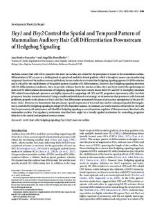
7.7 Activity 3: Calculating H-Complexity This section derives the formula for calculating H-complexity of a language (i.e. a domain) by counting the number of H sets, |H|. Firstly we calculate the number of H sets permitted by a single unary relation, and then a single relation of arbitrary arity. We then observe that binary relations (and higher) admit an infinite number of H sets, making H-complexity unusable. To overcome this we employ restrictions on the query language to calculate the number of basic queries that can be expressed for a set of relations. We then show that basic queries are not jointly exhaustive and pairwise disjoint (JEPD) and so do not correspond to H sets. Thus, we finally calculate H complexity as the smallest number of unique JEPD queries that can be expressed using combinations of basic queries. Initially, assume that all relations have an arity of 1 (i.e. they represent qualitative properties such as round or large). Tuples can take one of |AR| states for a relation R (such as holds), hence the complexity of a unary relation is |HR|=|AR|. However, once relations have an arity greater than 1 there are an infinite number of potential H sets, because a binary relation constitutes a total order. We proceed in our analysis by using a graph to represent a scenario that consists of a single binary relation Ri, where objects represent vertices and directed edges represent tuples as illustrated in Figure 5.
R1={ (a,b), (c,b)} R2={(a,a), (a,b), (b,c), (d,d), (d,e), (e,c)}
a
a
R3={(a,b), (c,d), (d,d), (e,f), (e,g), (g,g)}
b
c a
b
d
e b
c
f e
c
d
g
Figure 5. Three graphs representing binary relations R1, R2 and R3. In R3, subgraphs {a,b} and {c,d} correspond to basic queries, where {e,f,g} contains more than one basic query as induced subgraphs. A set theoretic query describes the structure of a graph and specifies the vertex to be selected with v bound variables (universally or existentially quantified), e.g. ... ∧ xv-1 ≠ xv. ∀x1...∃xv ⋅ x1 ≠ x2 ∧ ... ∧ x1 ≠ xv ∧ For brevity, we will omit explicitly stating these quantifications and conditions for all further queries, and for simplicity the variables in our examples are only existentially quantified. For example, the query {x2| (x1,x2)∈R1 ∧ (x3,x2)∈R1} will access b from the graph of R1 in Figure 5. While there are an infinite number of potential graphs and unique accessible subsets, homogeneous sets still exist that contain indistinguishable objects. Indeed, homogeneous sets correspond to graph symmetries. For example, regarding the graph of R1, no query exists that can separate objects a and c (without directly referring to those objects), {a,c} ={x1| (x1,x2)∈R1 ∧ (x3,x2)∈R1} ={x3| (x1,x2)∈R1 ∧ (x3,x2)∈R1}, and the graph of R2 has three H sets, accessed by the query {xi | (x1,x1)∈R2 ∧ (x1,x2)∈R2 ∧ (x2,x3)∈R2 ∧ (x4,x4)∈R2 ∧ (x4,x5)∈R2 ∧ (x5,x3)∈R2 }, namely {a,d} when i=1 or 4, {b,e} when i=2 or 5 and {c} when i=3. Given a graph of a scenario, the number of H sets is the number of vertices minus the number of symmetries. However, to make |HR| a function of the entire QSTR application language, rather than just isolated scenarios (i.e. rather than particular graphs), we apply the concept of restricted query languages from finite model theory (normally used for studying descriptive complexity (Marker, 2002)). If the restricted query language only recognises a finite number of graphs, it will admit a finite number of H sets. It is then possible to quantify the complexity of a relation independent of a particular scenario, and measure the relative difference in expressiveness between two languages. One common query restriction is to limit the number of variables (vertices). Previously, queries have referred to variables xi where i can be any positive integer. For example, if i≤2 then the allowable tuples are (x1,x1), (x1,x2), (x2,x1), and (x2,x2). If v is the number of variables allowed in a query, and aR is the arity of relation R (i.e. the size of the tuples) then for each query, the number of tuples is v↑aR. We refer to these queries as basic queries. For example, if v=2 then one basic query on a binary relation is {x1 | (x1,x1)∈R− ∧ (x1,x2)∈R+ ∧ (x2,x1)∈R− ∧ (x2,x2)∈R−}. Each tuple can be assigned to one of |ΑR| relation states, thus, the number of unique basic queries for relation R is |ΑR|number of tuples, where number of tuples = v↑aR.
Previously we only referred to one relation within a query. Given v bound variables, queries will now take the form, {x1 | query R1, query R2, …, query Rn}, where query Ri is one of the unique basic queries for relation Ri. Hence, the total number of queries permitted over n relations is |basic R1 queries| × … × |basic Rn queries|. Moreover, each query variable can be either existentially or universally quantified, i.e. the query can use any one of the combinations from v ∃x1∃x2…∃xv to ∀x1∀x2…∀xv. In general, the number of allowable variable quantifications q is 2 if all combinations are acceptable. Thus the number of unique basic relations including the acceptable variable quantifications is q × |basic R1 queries| × … × |basic Rn queries|. For H sets to truly represent the maximum refinement possible, they must be JEPD so that every object in a scenario will appear in exactly one H set. This property is critical; if it did not hold then further refinements could be achieved by taking H set intersections and differences. Basic queries are not necessarily JEPD (specifically, when their corresponding graphs are overlapping induced subgraphs of the full scenario graph) and so they do not specify H sets. For example, consider the scenario graph R3 in Figure 5. If v=2 then two basic queries are: {x1 | (x1,x1)∈R− ∧ (x1,x2)∈R+ ∧ (x2,x1)∈R− ∧ (x2,x2)∈R−}={a,e}, {x1 | (x1,x1)∈R− ∧ (x1,x2)∈R+ ∧ (x2,x1)∈R− ∧ (x2,x2)∈R+}={c,e}. Vertex e appears in both results, and therefore the basic queries are not JEPD. To calculate |H| we must determine the smallest JEPD queries that contain the basic queries. This is achieved by taking all combinations of basic queries by intersection and difference, hence |H|=2number of unique basic queries – 1 (we can ignore the trailing‘−1’). To summarise, • the language being measured has a set of relations R, • AR is the number of relation states allowed for relation R (such as holds and does not hold), • aR is the arity of relation R (e.g. binary relations have arity 2), • v is the number of variables allowed in a query (1 ≤ v), v • q is the number of variable quantifications (1 ≤ q ≤ 2 ), and • H is the set of H sets, and |H| is the H-complexity of the language. The formula for calculating H-complexity is
|H| = 2↑(q × |basic R1 queries| ×… × |basic Rn queries|) = 2↑( q (|AR1|↑v↑aR1) ×…× (|AR n|↑v↑aR n) ) = 2↑ (q ∏R∈R (|AR|↑v↑aR)).
(1)
7.8 Activity 3: Calculating H-Complexity For Refined Test Spaces The complexity of a language can be calculated simply by applying the formula in the previous section. However, once the designer has specified conditions for refining the test space, the formula can no longer be used. In this section we present a method for calculating the refined test space complexity by encoding it as a constraint satisfaction problem (CSP). The designer can then use any standard CSP solver, such as JaCoP (Kuchcinski, 2003), to calculate the complexity. A CSP is a finite number of variables (where each variable has a finite domain), and a set of constraints between variables. In our case, given a domain of relations R and the number of allowable query variables v, the CSP solver will return the number of basic queries permitted,
∏R∈R |basic R queries|. Equation 1 from the previous section can then be used to calculate the refined test space complexity. We now present our CSP encoding. Each variable represents a tuple from a basic query. From the previous section, the number of tuples for relation R is v↑aR. Let integers 1,2,3,4 represent holds, does not hold, not applicable, and indefinite respectively. For each relation R, declare v↑aR variables with domain AR, encoded as the appropriate subset of {1,2,3,4}. Next, specify the refinement conditions from Section 7.6. Finally, execute the solver and have it return the number of solutions (there is no need to record the solutions). If computation is not too time consuming, the solver can be executed multiple times to determine the impact of each constraint. Do this by executing the solver with only one constraint at a time, and record the different complexities. Alternatively, execute the solver with all but one constraint (for each constraint) to quickly determine whether any constraints are redundant. For example, given the domain R={light, room, warm, in}, v=2 allowable query variables, and for every relation AR={+,−,~,?}, q=1 variable quantification (both variables existentially quantified), the number of basic queries is q ∏R∈R (|AR|↑v↑aR) = (4↑2↑1) (4↑2↑1) (4↑2↑1) (4↑2↑2) = 16⋅16⋅16⋅256 = 1 048 576, yielding a completely intractable test space, with complexity |H| = 2↑1048576. A designer then refines this test space by specifying the following conditions: • only test when x is a light and y is a room • because both object types are assumed, ignore the not applicable relation state (all relations apply for lights and rooms) the types light and room are mutually exclusive • • in is not reflexive • in is not symmetric • nothing is ever in a light The designer then encodes the CSP problem1 using JaCoP (Kuchcinski, 2003). Firstly the variables are declared, using a restricted domain that excludes not applicable. Store network = new Variable light_x Variable light_y Variable room_x Variable room_y Variable warm_x Variable warm_y Variable in_x_x Variable in_y_y Variable in_x_y Variable in_y_x 1
Store(); = new Variable(network, = new Variable(network, = new Variable(network, = new Variable(network, = new Variable(network, = new Variable(network, = new Variable(network, = new Variable(network, = new Variable(network, = new Variable(network,
“light_x”, domain(1,2,4)); “light_y”, domain(1,2,4)); “room_x”, domain(1,2,4)); “room_y”, domain(1,2,4)); “warm_x”, domain(1,2,4)); “warm_y”, domain(1,2,4)); “in_x_x”, domain(1,2,4)); “in_y_y”, domain(1,2,4)); “in_x_y”, domain(1,2,4)); “in_y_x”, domain(1,2,4));
Here we have explicitly enumerated variables and constraints for clarity. In practice, generator methods should be used that accept a set of relation names, domains AR, and the number of query variables v, and return the set of variables. Convenience methods should also be created that accept relation names, parameter patterns, and a constraint type, and impose the appropriate set of constraints (rather than explicit enumeration). Please contact the first author (
[email protected]) for a Java implementation of an H complexity calculator.
Next, the designer encodes the constraints. //- only test when x is a light and y is a room network.impose( new XeqC(light_x, 1) ); network.impose( new XeqC(room_y, 1) ); //- types “light” and “room” are mutually exclusive network.impose( new IfThen( new XeqC(light_x, 1), new XeqC(room_x, 2)) ); network.impose( new IfThen( new XeqC(light_y, 1), new XeqC(room_y, 2)) ); network.impose( new IfThen( new XeqC(room_x, 1), new XeqC(light_x, 2)) ); network.impose( new IfThen( new XeqC(room_y, 1), new XeqC(light_y, 2)) ); //- "in" is not reflexive network.impose( new XeqC(in_x_x, 2) ); network.impose( new XeqC(in_y_y, 2) ); //- "in" is not symmetric network.impose( new IfThen( network.impose( new IfThen(
new new new new
//- nothing is ever "in" a “light” network.impose( new IfThen( new new network.impose( new IfThen( new new
XeqC(in_x_y, XeqC(in_y_x, XeqC(in_y_x, XeqC(in_x_y,
1), 2)) ); 1), 2)) );
XeqC(light_x, 1), XeqC(in_y_x, 2)) ); XeqC(light_y, 1), XeqC(in_x_y, 2)) );
Next, the designer runs the solver which returns 27 solutions. The test space of size 227 is now practical for certain important coverage metrics, although further refinements can be made, for example, choosing to only test one room at a time (Schultz et al., 2009). The designer executes the solver multiple times, each run using only one of the constraints, and determines that constraints 1 and 4 have the most impact. Once again the designer executes the solver multiple times, each run using all but one constraint (for each constraint) and determines that some constraints are redundant and can be removed such as network.impose( new IfThen(
new XeqC(light_y, 1), new XeqC(room_y, 2)) );
Note that, after removing one constraint, the process should be repeated rather than removing multiple constraints at once.
7.9 Activity 4: Calculate The Class of a Given Test Instance To determine the test coverage of a given set of tests, the designer must compare the tests to the test space in terms of H-complexity. That is, the designer needs to determine which combination of H sets are exercised in a given test. A test is a set of input premises and expected outputs. The input premise information is a set of relations that contain object tuples, such as within+={(a,b), (b,c)}, school+={a}, Downtown+={b}, Auckland+={c}, near−={(c,d)}, within?={(a,c)}. By convention, for each
relation, any unspecified tuples can be assumed to be in the indefinite relation state (e.g. Auckland?={a,b,d}). The expected output is again a set of relations that contain object tuples, such as within+={(a,b), (b,c), (a,c)}. A test is satisfied by a QSTR application if, given the premises, reasoning produces a scenario that satisfies the expected outputs. Given a domain being tested and a test instance, the designer needs to determine which test class the given test is in with respect to the domain’s test space. Using H sets we define a test class as the premise scenario specified in the test (that is, we ignore the expected output). To calculate the class of a given test we use a CSP encoding. To summarise, query variables and scenario objects are encoded. CSP is then used to select every possible combination of scenario objects for the query variables, and for each combination it constructs the H set from the relation states for the particular chosen objects. Firstly, we use an integer coding system for representing each unary object tuple, binary object tuple, and so on, up to each n-ary tuple. The following integer coding is one example of how this can be accomplished. The greatest tuple arity (i.e. the n-ary tuples) required to express the scenario is equal to the greatest relation arity; in the above example the greatest relation arity is 2. Thus, given a scenario with n objects, let integers 0 to n−1 represent each object. Next, let integers n to 2n−1 represent tuples (0,0), (0,1),…,(0,n−1), integers 2n+1 to 3n−1 represent tuples (1,0), (1,1),…, (1,n−1), and so on; hence, n2 binary tuples are represented by integers n to n+n2−1. The relationship between the object identifiers and the tuple identifier is (x+1)n+y (that is, the last tuple is represented by the integer (n−1+1)n+n−1= n+n2−1). Secondly, for each allowable tuple of query variables, create one CSP variable, with domains of values representing every object tuple of the appropriate arity. For example, if v=2 then six variable tuples are required. Variable x = new Variable(store, “x”, 0, n-1) Variable y = new Variable(store, “y”, 0, n-1) Variable x_x = new Variable(store, “x_x”, n, n*n+n-1) Variable x_y = new Variable(store, “x_y”, n, n*n+n-1) Variable y_x = new Variable(store, “y_x”, n, n*n+n-1) Variable y_y = new Variable(store, “y_y”, n, n*n+n-1)
Impose the constraint that the variables are not equal to ensure that they represent different objects in each solution. store.impose(new Alldifferent(new Variable[]{x,y})); store.impose(new Alldifferent(new Variable[]{x_x,x_y,y_x,y_y}));
Thirdly, encode the basic queries in terms of H sets using the method from the previous section. That is, for each tuple from a basic query of relation R, create a variable with a domain that represents the allowable tuple states AR, i.e. some subset of {1,2,3,4} where integers 1,2,3,4 represent holds, does not hold, not applicable, and indefinite respectively. Do not encode the test space refinement constraints. Finally, link the scenario encoding to the basic query encoding. For each relation, create an implication constraint that associates the object tuple selected by the query variables to the relation state in the H set. For example, encoding within+={(a,b), (b,c)}, where a=0, b=1, c=2, d=3, (a,b)=5 and (b,c)=10 requires the following constraint.
store.impose(new IfThenElse( new Or(XeqC(x_y,5), XeqC(x_y,10)),
//- if variable matches a tuple
new XeqC(within_x_y,1),
//- then H set relation state holds
new XeqC(within_x_y,2)));
//- else relation state does not hold
Note that further nested IfThenElse constraints are required to also explicitly specify the not holds, not applicable and indefinite states. Execute the solver to get all solutions. The class of a test is determined by the set of solutions for the basic query encoding variables, and the value of the object variables that satisfy those basic queries. Once the designer knows the class that each test is in (that is, the combination of H sets from which objects are specified), they can run the test coverage metrics presented in the following section.
7.10 Activity 5: Test Coverage Metrics This section presents four test coverage metrics based on H-complexity. To illustrate the test coverage metrics we will use the following running example. Let the domain being tested contain one binary relation R that can take two states AR={+,−}. Two query variables are allowed, v=2 and one variable quantification, q=1. The number of query tuples is v↑aR=22=4, which are (x1,x1)∈R, (x1,x2)∈R, (x2,x1)∈R, and (x2,x2)∈R. The number of basic queries is q ∏R∈R (|AR|↑v↑aR)=1⋅24=16, which are b1={x1 | (x1,x1)∈R+ ∧ (x1,x2)∈R+ ∧ (x2,x1)∈R+ ∧ (x2,x2)∈R+}, b2={x1 | (x1,x1)∈R+ ∧ (x1,x2)∈R+ ∧ (x2,x1)∈R+ ∧ (x2,x2)∈R−}, b3={x1 | (x1,x1)∈R+ ∧ (x1,x2)∈R+ ∧ (x2,x1)∈R− ∧ (x2,x2)∈R+}, … b16={x1 | (x1,x1)∈R− ∧ (x1,x2)∈R− ∧ (x2,x1)∈R− ∧ (x2,x2)∈R−}. The number of H sets is |H| = 2↑(q ∏R∈R (|AR|↑v↑aR))=216. The number of scenario classes is 2|H|=2↑(216). Let the example test set consist of two tests with the following H sets • test t1: (b1, b2) • test t2: (b1), (b2,b3). Our four test coverage metrics, strictly ordered in terms of coverage strength (from weakest to strongest) are • tuple state coverage (TS), • basic query coverage (BQ), • H set coverage (H), and • scenario coverage (S). Tuple state (TS) coverage measures the number of query tuples that have taken a particular state in at least one test. Full TS coverage means that every query tuple has been assigned to every allowable relation state in at least one test. This should be viewed as an absolute minimum coverage requirement that all QSTR application test sets must satisfy. The total number of tuples with states that a language admits is ∑R∈R |AR| ⋅ (v↑aR). In the running example there are 4 query tuples, and each tuple can take 2 states, giving 2⋅4=8 possible tuples with states, namely (x1,x1)∈R+, (x1,x2)∈R+, (x2,x1)∈R+, (x2,x2)∈R+, (x1,x1)∈R−, (x1,x2)∈R−, (x2,x1)∈R−, (x2,x2)∈R−. The example test set contains the following tuples (x1,x1)∈R+, (x1,x2)∈R+, (x2,x1)∈R+ , (x2,x2)∈R+, (x2,x1)∈R− , (x2,x2)∈R−. Hence percent TS coverage is 5/8=62.5%.
Basic query (BQ) coverage measures the number of basic queries that have appeared in at least one test. Full BQ coverage means that every basic query has been used to describe some test scenario. While stronger than full TS coverage, full BQ coverage should also be viewed as a minimum coverage requirement for application validation. In the running example, the test set contains 3 basic queries (b1, b2, b3), giving a percent BQ coverage of 3/16=18.75%. H set (H) coverage measures the number of H sets that have been used to specify scenarios in at least one test. In practice, full H coverage is often very difficult to achieve, as it constitutes a vast class of tests. Instead the designer should focus on satisfying important subclasses within full H coverage, discussed below. The running example test set has 3 H sets, giving a percent H coverage of 3/(216)≈0%. Scenario (S) coverage measures the number of scenario classes exercised in at least one test, where a scenario class is some unique combination of H sets from which objects in the class of scenarios are drawn. In practice full S coverage is impossible to achieve, except for trivially small domains. However, after test space refinement S coverage can be a useful measure. In the running example two scenario classes are exercised, namely {(b1, b2)} and {(b1), (b2,b3)}. This gives a percent S coverage of 2/(2↑216)≈0%. Full BQ coverage is trivially easy to achieve, for example full BQ coverage is satisfied by one test where the scenario returns objects from all 16 basic queries. On the other hand, achieving full H coverage is often difficult in practice, and achieving full S coverage is, in almost all cases, impossible. Our current research is focused on identifying valuable classes within this test space in terms of H and S coverage. For example, two potentially significant H coverage criteria are • all H sets that consist of exactly one basic query, and • all H sets that consist of exactly two basic queries The first class of tests will ensure that all basic queries have been exercised in isolation (giving full TS and BQ coverage). The second class ensures that the interactions between all pairs of basic queries have been exercised. Both of these test classes are relatively small and often practical to achieve. If the number of basic queries is b then the test class sizes are b and b(b−1) respectively, where the maximum size of b is (q ∏R∈R (|AR|↑v↑aR)).
8.0 FUTURE RESEARCH Our long term aim is to develop a QSTR application development environment inspired by Garp3 and other UML software tools. This will be used for designing, validating and automatically implementing the reasoning component of a QSTR application, and will integrate software tools that support the methodologies discussed in this chapter. The workbench will allow the designer to easily employ existing QSTR libraries such as SparQ and GQR, structure their application by declaring fragments and design patterns such as fragment definitions, derive high level neighbourhoods, automatically generate tests from critical test classes, and execute validation metrics such as test coverage. Additionally, a suite of metrics will be available that analyse an application based on external test data, e.g. using classification techniques on test data to analyse the quality of a designer’s fragment definitions. Once a QSTR application design has been finalised, our workbench will generate a standalone implementation, such as a jar file, that will accept a scenario description and perform the required task, such as envisioning. We are also planning to compile a library of application contexts, such as a qualitative GIS suite, an office environment suite, a sports field suite, architectural lighting suite, and so on. Each
library component would consist of the relevant existing QSTR calculi, along with other standard high level commonsense relations and rules.
9.0 CONCLUSIONS A number of critical barriers to QSTR application development must be addressed, namely that the important characteristics of QSTR problems need to be defined, QSTR application designers need to develop task specific qualitative relations and constraints, there are no methodologies for developing or analysing QSTR applications, and that application designers will typically be software engineers rather than logicians. In this chapter we address these problems with a collection of methodologies that support the design and validation of QSTR applications. We established a theoretical foundation for QSTR applications, and used this to define the roles of application designers and users, and to identify three fundamental QSTR application operations, selection, insertion, and scenario universe modification. We presented four central properties of QSTR applications, specifically, reasoning across a broad range of abstraction levels, continuity assumption, modelling infinite domains, and reasoning about objects in multi-dimensional models. Our methodologies for QSTR application development focused on supporting the designer in three of these key areas. We adapted two standard formal requirements from software engineering for QSTR applications, which were the customer’s operational requirements and functional requirements. We presented critical characteristics of QSTR problems based on our theoretical foundations of QSTR applications and a review of existing QSTR literature, and showed how these characteristics determine the customer’s operational profile. We enumerated a set of significant purely qualitative tasks that defines the exact extent to which QSTR can be applied, and we established a template that covers all general QSTR application behaviour sequences in a UML state diagram. QSTR applications are organised into groups of relations, called fragments. We presented two design patterns, fragment definitions and fragment generalisations, for structuring fragments. We presented a methodology for defining high level neighbourhoods that are consistent with the structure of fragments in a QSTR application. For this we defined two novel components of conceptual neighbours, path restrictions and transition equivalence classes, and showed how the designer can use these to customise a derived high level neighbourhood graph. Finally, we presented a novel methodology for QSTR application validation, inspired by research in software engineering and finite model theory. We defined a complexity metric called H-complexity, and developed test coverage metrics for assessing the quality of unit and integration test sets.
REFERENCES Allen, J. F. (1983). Maintaining knowledge about temporal intervals. Communications of the ACM. 26 (11) (pp. 832-843). ACM Press. Bhatt, M. (2007) A Causal Approach for Modelling Spatial Dynamics: A Preliminary Report. Proceedings of the Workshop on Spatial and Temporal Reasoning, 20th International Joint Conference on Artificial Intelligence (IJCAI-07).
Bredeweg, B., Bouwer, A., Jellema, J., Bertels, D., Linnebank, F. & Liem, J. (2007) Garp3: a new workbench for qualitative reasoning and modelling. Proceedings of the 4th international conference on Knowledge Capture (K-CAP’07) (pp. 183-184). Burnstein, I. (2003). Practical software testing: a process oriented approach. Springer, New York. Cohn, A. (2008) Conceptual Neighborhood. Definition in Shekhar, S., Xiong, H., Encyclopedia of GIS (pp. 123). SpringerScience, New York, United States of America. Cohn, A. G., & Renz, J. (2008). Qualitative Spatial Representation and Reasoning. In van Hermelen, F., Lifschitz, V., Porter, B. (Eds), Handbook of Knowledge Representation (pp. 551-596). Elsevier. Cunningham, W. (1995), About the Portland form. http://c2.com/ppr/about/portland.html [Available: 8 August 2009]. Dylla, F. & Wallgrün, J.O. (2007). Qualitative Spatial Reasoning with Conceptual Neighborhoods for Agent Control. In Journal of Intelligent and Robotic Systems, 48 (1) (pp. 55-78). Dylla, F., Frommberger, L., Wallgrün, J. O. & Wolter, D. (2006). SparQ: A Toolbox for Qualitative Spatial Representation and Reasoning. Proceedings of the Workshop on Qualitative Constraint Calculi: Application and Integration. Freksa C. (1992), Temporal reasoning based on semi-intervals, Artificial Intelligence, 54, pp. 199–227. Gantner, Z., Westphal, M. & Wölfl, S. (2008). GQR - A Fast Reasoner for Binary Qualitative Constraint Calculi. Proceedings of the AAAI'08 Workshop on Spatial and Temporal Reasoning (pp. 24-29), Chicago, United States of America. Guesgen, H. W. (2002) “Fuzzifying Spatial Relations”. Applying soft computing in defining spatial relations, Matsakis P. and Sztandera L. (Eds.), Physica-Verlag, Hei-delberg, Germany, pp.1-16. Hodges, W. (1997) A Shorter Model Theory. Cambridge University Press. Iwasaki, Y. (1997) Real-World Applications of Qualitative Reasoning. IEEE Expert 12(3) (pp. 16-21). Kuchcinski, K. (2003) Constraints-driven scheduling and resource assignment. ACM Transactions on Design Automation of Electronic Systems (TODAES), 8(3) (pp. 355-383). Li, J. J., Huang, J. & Renz, J. (2009). A Divide-and-Conquer Approach for Solving Interval Algebra Networks. Proceedings of the 21st International Joint Conference on Artificial Intelligence (IJCAI 2009) (pp. 572- 577), Pasadena, United States of America. Ligozat, G., Mitra, D. & Condotta, J. (2004). Spatial and temporal reasoning: beyond Allen’s calculus. AI Communications 17(4) (pp. 223–233). Marker, D. (2002) Model Theory: An Introduction. Springer Verlag New York. Nebel, B., & Bürckert, H. J. (1995). Reasoning about temporal relations: A maximal tractable subclass of Allen’s interval algebra. Journal of the ACM 42(1) (pp. 43-66).
Pooley, R. J. (2004) Applying UML advanced application. Elsevier, Oxford. Qayyum, Z.U. & Cohn, A.G. (2007) Image retrieval through qualitative representations over semantic features. Proceedings of the 18th British Machine Vision Conference (BMVC2007) (pp. 610-619). Renz, J. (1999). Maximal Tractable Fragments of the Region Connection Calculus: A Complete Analysis. Proceedings of the 16th International Joint Conference on Artificial Intelligence (IJCAI'99) (pp. 448-455), Stockholm, Sweden. Renz, J. (2007). Qualitative Spatial and Temporal Reasoning: Efficient Algorithms for Everyone. Proceedings of the 20th International Joint Conference on Artificial Intelligence (IJCAI-07) (pp. 526-531), Hyderabad, India. Schultz, C., Amor, R. & Guesgen, H.W. (2009) Unit Testing for Qualitative Spatial and Temporal Reasoning. Proceedings of the 22nd Florida Artificial Intelligence Research Society Conference (FLAIRS-22), Sanibel Island, United States of America. Schultz, C., Clephane, T.R., Guesgen, H.W. & Amor, R. (2006) Utilisation of qualitative spatial reasoning in geographic information systems. Proceedings of the International Symposium on Spatial Data Handling (SDH-06) (pp. 27-42), Vienna, Austria. Schultz, C., Guesgen, H.W. & Amor, R. (2007) A system for querying with qualitative distances in networks. Proceedings of the IEEE International Conference on Fuzzy Systems (FUZZ-IEEE'07) (pp. 640-645), London, England. SETC - Software Engineering Technical Committee, (1984) IEEE guide to software requirements specifications, IEEE Computer Society, New York, United States of America. Van de Weghe, N., Cohn, A.G., De Tré, G. & De Maeyer, P. (2006) A Qualitative Trajectory Calculus as a Basis for Representing Moving Objects in Geographical Information Systems. Control and Cybernetics 35(1) (pp. 97-119). Westphal, M. & Wölfl, S. (2009). Qualitative CSP, finite CSP, and SAT: Comparing methods for qualitative constraint-based reasoning. Proceedings of the 21st International Joint Conference on Artificial Intelligence (IJCAI 2009) (pp. 628-633), Pasadena, United States of America. Wölfl, S., Mossakowski, T. & Schröder, L. (2007) Qualitative constraint calculi: Heterogeneous verification of composition tables. In Proceedings of the 20th International Florida Artificial Intelligence Research Society Conference (FLAIRS 2007) (pp. 665-670). AAAI Press. Zhu, H., Hall, P. A. V. & May, J. H. R. (1997) Software unit test coverage and adequacy. In ACM Computing Surveys (CSUR), 29(4) (pp. 366-427), ACM New York, United States of America.
KEY TERMS & DEFINITIONS Application designer: determines the QSTR application language and model, given formal software requirements.
Validation: process conducted to ensure that a software system is fit for purpose. Complexity: a measure of the expressiveness of a relational language; specifically, the number of distinct scenarios that can be represented. Requirements: the necessary properties of the intended application for that application to have value, such as characteristics of the domain being modelled, the tasks that the intended system needs to be capable of performing, and the system’s behaviour during runtime. Neighbourhood: a graph where vertices represent relations are edges represent conceptual neighbours; two relations are conceptual neighbours if it is possible for a tuple of objects to transition between those relations without requiring a third, intermediate relation. Test coverage: the proportion of a selected class of software components exercised by a test suite. QSTR applications: a class of relational systems, typically characterised by modelling a broad range of abstraction levels, modelling continuity in dynamic scenarios, and modelling infinite, partially ordered domains.