existing tools, petrify represents the encoded specification as an. STG, and thus .... The following two properties of insertion sets, based on theory .... In the current implementation, the complexity of the circuit is ap- ... reasonable amount of memory or time by SIS or ASSASSIN. ... Integration: the VLSI journal, 4:99â113, 1986.
Methodology and tools for state encoding in asynchronous circuit synthesis � Jordi Cortadella, Univ. Politecnica de Catalunya, Barcelona, Spain Michael Kishinevsky, Alex Kondratyev, The University of Aizu, Japan Luciano Lavagno, Politecnico di Torino, Italy Alex Yakovlev, University of Newcastle upon Tyne, United Kingdom
Abstract This paper proposes a state encoding method for asynchronous circuits based on the theory of regions. A region in a Transition System is a set of states that “behave uniformly” with respect to a given transition (value change of an observable signal), and is analogue to a place in a Petri net. Regions are tightly connected with a set of properties that must be preserved across the state encoding process, namely: (1) trace equivalence between the original and the encoded specification, and (2) implementability as a speedindependent circuit. We build on a theoretical body of work that has shown the significance of regions for such property-preserving transformations, and describe a set of algorithms aimed at efficiently solving the encoding problem. The algorithms have been implemented in a software tool called petrify. Unlike many existing tools, petrify represents the encoded specification as an STG, and thus allows the designer to be more closely involved in the synthesis process. The efficiency of the method is demonstrated on a number of “difficult” examples.
1 Introduction In the last decade, Signal Transition Graphs (STGs) [7, 1] have attracted much of the attention of the asynchronous circuit design community due to their inherent ability to capture the main paradigms of asynchronous behaviour: causality, concurrency and data-dependent and non-deterministic choice. STGs are Petri nets whose events are interpreted with signal transitions of a modeled circuit. The STG model, exactly like “classical” Flow Table models, may require some state signals to be added to those initially specified by the designer. Adding those state signals is commonly referred to as solving the Complete State Coding (CSC) problem. Since [1] a number of different techniques have been proposed to solve the CSC-problem. The first totally general method, described in [8], used an algorithm whose complexity practically precluded any optimization, but produced only one,often suboptimal, solution. The most recent method [9] is based on the concept of an excitation � This work has been partially supported by grant CICYT TIC 95-0419 (J. Cortadella), EPSRC visiting fellowship GR/J78334 (M. Kishinevsky), MURST project “VLSI architectures” (L. Lavagno), and EPSRC grant GR/J52327 (A. Yakovlev).
region for a signal transition (a set of states in which a signal is enabled to change its value). It has been able to improve on [8] by adopting a coarser granularity in the exploration of the solution space. This coarser granularity has a price, though: as we will show in Section 6, there is a number of examples of STGs which could not be solved by their method (nor by previous ones, mainly due to the large number of states), unless changes in the specification (e.g., reductions in concurrency) are allowed. Moreover, the authors could not characterize the class of STGs for which their method was guaranteed to find a solution. Our approach differs from the previous work in the area, because it is based on the notion of regions of states, which is more general than, albeit related to, that of excitation regions (an excitation region is a specific intersection of regions). By exploring a broader design space than [9], we can thus solve a larger number of problems, and potentially reach better solutions especially in terms of circuit performance. For example, our approach can efficiently trade off logic complexity with execution speed, by changing the level of parallelism with which state signal transitions are inserted. On the other hand, our search space is still reduced with respect to [8], and thus we can claim better control on the quality of the solution. This paper is organised as follows. Section 2 provides some theoretical background (the interested reader is referred to [2] for the details). Sections 3 and 4 define the idea of property-preserving event insertion and apply it to solving the CSC problem. Sections 5 and 6 describe implementation aspects and experimental results.
2
Theoretical background
2.1
Transition systems and Petri nets p1
p2
s1
a
a
b
s2
s3
c
c
s4
s5
a
b
p4
p1p3p5 c p1p4
p5
a
b c
s6
(a)
p2p3p5 c p2p4
p3
a
b
p1p2p4p5 b
(b)
p3 (c)
Figure 1: A TS (a), the corresponding PN (b), its RG (c) Informally, a TS ([6]) can be represented as an arc-labeled directed graph. A simple example of a TS without cycles is shown in Figure 1,a. A TS is called deterministic if for each state s and each 33rd Design Automation Conference Permission to make digital/hard copy of all or part of this work forpersonal or class-room use is granted without fee provided that copiesare not made or distributed for profit or commercial advantage, thecopyright notice, the title of the publication and its date appear,and notice is given that copying is by permission of ACM, Inc. Tocopy otherwise, to republish, to post on servers or to redistribute tolists, requires prior specific permssion and/or a fee. DAC 96 - 06/96 Las Vegas, NV, USA 1996 ACM, Inc. 0-89791-833-9/96/0006..$3.50
label a there can be at most one state s0 such that s s0 . A TS is called commutative if whenever two actions can be executed from some state in any order, then their execution always leads to the same state, regardless of the order. A Petri Net is a quadruple N = (P;T; F; m0 ), where P is a finite set of places, T is a finite set of transitions, F (P T ) (T P ) is the flow relation, and m0 is the initial marking. A transition t T is enabled at marking m1 if all its input places are marked. An enabled transition t may fire, producing a new marking m2 with one less token in each input place and one more token in each output t place (m1 m2 ). A PN expressing the same behavior as the TS from Figure 1,a is shown in Figure 1,b. The set of all markings reachable in N from the initial marking m0 is called its Reachability Set. A net is called safe if no more than one token can appear in a place in any reachable marking. The graph with vertices corresponding to markings of a PN and with an arc (m1 ; m2 ) in the graph if and only if m1 m2 is called its Reachability Graph (RG). One can easily check that the RG Figure 1,c derived for the PN from Figure 1,b is isomorphic to the TS (Figure 1,a).
!a
�
d
)
62 !
f
!
62
g
! b this set, while another transition also labeled with b, s4 ! s6 , does f
g
not. A region r is a pre-region of event e if there is a transition labeled with e which exits r. A region r is a post-region of event e if there is a transition labeled with e which enters r. The set of all pre-regions and post-regions of e is denoted with � e and e� respectively. While regions in a TS are related to places in the corresponding PN, an excitation region for event a is a maximal set of states in which transition a is enabled. Therefore, excitation regions are related to transitions of the PN. A set of states is called an excitation region for event a (denoted by ERj (a)) if it is a maximal connected set of states such that for every state s ERj (a) there is a transition s a . Since any event a can have several separated ERs, an index j is used for the distinction between different connected occurrences of a in the TS. In the TS from Figure 1,a there are two excitation regions for event a: ER1 (a) = s1 and ER2 (a) = s5 . Similarly to ERs, we define switching regions as connected sets of states reached immediately after the occurrence of an event.
2
!
f g
f g
3 Property-preserving event insertion Event insertion is informally seen as an operation on a TS which selects a subset of states, splits each state in it into two states and creates, on the basis of these new states, an excitation and switching region for a new event. Figure 2 shows the chosen insertion scheme, analogous to that used by most authors in the area, in the three main cases of insertion with respect to the position of the states in the insertion set ER(x) (entrance to, exit from or inside ER(x)).
c x
c
b x
b
x
x
a
!
8 2
2
!^
!
2
2
Regions and Excitation Regions
2
x
State signal insertion must also preserve the speed-independence of the original specification, that is required for the existence of a hazard-free asynchronous circuit implementation. An event a of a TS A is said to be persistent in a subset S 0 of states of S iff s1 S 0 ; b E : [s1 a (s1 b s2) a T ] s2 . An event is said to persistent if it is persistent in S . For a binary encoded TS, determinism, commutativity and output event persistency guarantee speed-independenceof its circuit implementation. Formally, we say that an insertion state set ER(x), in a TS A0 obtained from a deterministic and commutative TS A by inserting event x, is a speed-independence preserving subset (SIPset) iff: (1) for each a E , if a is persistent in A, then it remains persistent in A0 , and (2) A0 is deterministic and commutative. The following two properties of insertion sets, based on theory developed in [2], link together the notions of TSregions and SIP-sets and provide a rationale for our approach.
!
� !
SR(x)
Figure 2: Event insertion scheme
!
2
d
a
ER(x)
� [ �
Let S1 be a subset of the states of a TS, S1 S . If s S1 a 0 and s0 S1 , then we say that transition s s enters S1 . If s S1 and s0a S1 , then transition s a s0 exits S1 . Otherwise, s0 does not cross S1 . A region is a subset of transition s states with which all transitions labeled with the same event e have exactly the same “entry/exit” relation. This relation will become the predecessor/successor relation in the Petri net. Let us consider the TS shown in Figure 1. The set of states r3 = s2; s3 ; s6 is a region, since all transitions labeled with a and with b enter r3 , and all transitions labeled with c exit r3 . On the b other hand, s2 ; s3 is not a region since transition s1 s3 enters
b
ER(x)
2
2.2
c
� � �
Property 3.1 (P1) If r is a region in a commutative and deterministic TS, then r is an SIP-set.
(P2) If r is an excitation region of an event a in a commutative and deterministic TS and a is persistent in r, then r is an SIP-set.
(P3) If r1 and r2 are pre-regions of the same event in a commutative and deterministic TS, r1 r2 is connected and all exit events of r1 r2 are persistent, then r1 r2 is a SIP-set.
\
\
\
These properties suggest that the good candidates for insertion sets should be sought on the basis of regions and their intersections (while the approach of [9] could exploit only case P2). Since any disjoint union of regions is also a region, this gives an important corollary that nice sets of states can be built very efficiently, from “bricks” (regions) rather than “sand” (states).
4
Solving Complete State Coding
A Signal Transition Graph (STG, [1, 7]) is a Petri net labeled with up and down transitions of a set of signals (denoted by x+ and x for signal x respectively). A necessary condition for STG implementability is consistent labeling. Informally, this means that in every firing sequence from the initial marking, rising and falling transitions alternate for each signal. In other words, each marking can be uniquely labeled with a vector of signal values. Once consistency is ensured,Complete State Coding (CSC) becomes necessary and sufficient for the existence of a logic circuit implementation. A consistent STG satisfies the CSC property if for every pair of states s; s0 of the associated TS, such that v(s) = v(s0 ), the set of non-input transitions enabled in both is the same. Assume that the set of states S in a TS is partitioned into two subsets which are to be encoded by means of an additional signal to solve some CSC conflicts. Let r and r = S r denote the blocks of such a partition. In order to implement such an encoding, we need to insert appropriate transitions of the new signals in the border states between the two subsets. In this paper we shall consider the so-called exit border (EB) of a partition block r, denoted by EB (r), which is informally a subset
of states of r with transitions exiting r. We call EB (r) well-formed if there are no transitions leading from states in EB (r) to states in r EB (r). Consider the example in Figure 3 (enabled signals have their value followed by in the signal label). State pair (1� 1; 1�1� ) has a CSC conflict, assuming that signal a is input and b is non-input, and so do (1�1; 1�1� ) and (0�1; 01� ) (while (00�; 0� 0� ) does not, because b is enabled in both). The partition r = r2; r = r20 separates all conflicting pairs, and can thus be tentatively used to solve the conflicts. The borders, in this case, are denoted by the shaded areas. If they are selected as excitation regions for the new signal y, we obtain the TS (c). Note that some border states are conflicting. This means that the new TS will still have secondary CSC problems, that must be solved by iterating the procedure (the proof of convergence is given in [2]).
�
r1
r2 a+
r1’
1*0* a-
r3
0*0*
b+
a+
r3’
r2’ a-
b01*
b-
b+
0*1 a+
a-
bEB(r2’)
1*1* b+
a-
1*0*0 a-
1*0*
b+
00*0* y+ b-
0*0*1
y=0 1*10 a-
a+
ya-
b+
00*1
a+
y-
a-
b-
1. Generate a set of I-partitions that preserve speed independence (figure 4) 2. Estimate the cost of the generated I-partitions
(d)
4. Increase the concurrency of the inserted signal y=1
(c)
Figure 3: Illustration of event insertion Note that we need each new signal x to orderly cycle through states in which it has value 0, 0�, 1 and 1� . We can formalize this requirement with the notion of I-partition ([8] used a similar definition). Given a TS TS = (S; T; E; sin ), an I-partition is a partition of S into four blocks: S 0 , S 1 , S + and S . S+0 (S 1 ) defines the states in which x will have the value 0 (1). S (S ) defines ER(x+) (ER(x )). For a consistent encoding of x, the only allowed events S+ crossing boundaries of the blocks are the following: S 0 S1 S S 0 , S + S and S S + (the latter two would cause a persistency violation, though). The problem of finding an I-partition is reduced to finding a bipartition S . Each block b of S induces a bipartition b; b , (b = S +b). Given a block b, an I-partition can be calculated by defining S and S with the following recursion:
!
!
!
!
!
2.
!
f g
n
1.
fs 2 b j 9 s ! s0 ^ s0 2 bg � S + fs 2 b j 9 s ! s0 ^ s0 2 bg � S + ^ s0 2 b ^ s ! s0 ] ) s0 2 S + [s 2 S [s 2 S ^ s0 2 b ^ s ! s0 ] ) s0 2 S
and finally S 0 = b
A heuristic-search strategy to solve CSC
3. Select the best I-partition
b+ 10*1
g g
;
5
1*11*
a-
[f [f
good blocks = good blocks new bl new frontier = new frontier new bl frontier = select the best FW blocks from new frontier until new frontier = return the best block in good blocks
The main algorithm for the insertion of one state signal is as follows:
b11*0
011* b+
y+
01*1
01*0 y-
2
new bl = bl [ br if cost(new bl) < cost(bl) then
(b)
010* y+
a+
;
by condition 1 correspond to the smallest “legal” exit border of b with respect to b (EB (b)). The additional states of condition 2 define the smallest well-formed EBs. We will denote by MWFEB(b) the minimal well-formed EB of b. The set of candidates explored by our encoding algorithm will be restricted to be an I-partition by construction. We proved in [2] that the method is complete, in that it can solve CSC for any safe, consistent, output-persistent STG.
EB(r2)
r2’ b+
2
g
Figure 4: Heuristic search to find a block for event insertion
1*1 a-
00*
(a)
f
r2
b+ b+
bricks = calculate all bricks () frontier = good blocks = the best FW bricks repeat /* heuristic search */ new frontier = for each bl frontier do for each br bricks adjacent to bl do
S + and S 1 = b S
. The sets of states defined
Initially, all bricks of the TS are calculated by (1) obtaining all minimal regions of the TS and (2) calculating all possible intersections of pre-/post-regions of the same event. Since the number of pre- and post-regions of an event is usually small, an exhaustive generation is feasible. The best block for event insertion is obtained as the union of adjacent bricks. At each iteration of the search, a frontier of FW (frontier width, a parameter trading off solution quality versus time) “good” blocks is kept. Each block is enlarged by adjacent bricks and the new obtained blocks are considered candidates for the next iteration only if they are “better”, according to the cost function, than their ancestors. The final block for insertion is calculated as the union of best disconnected blocks. A greedy block merging approach guided by the cost function is used. Given a block b, S + and S are initially calculated as the MWFEB of b and b respectively. This leads to a solution with minimum concurrency of the inserted event. Concurrency can be increased by enlarging S + and/or S ([8]). In our approach, after having calculated the best configuration for event insertion, S + and S are greedily enlarged by adding bricks that are adjacent to them. The enlargement is only accepted if the new configuration improves the cost of the solution. The following factors are considered in the cost function for the insertion of signal x (in order of priority):
� �
ER(x+) and ER(x ) must be SIP blocks.
The insertion of x must not modify the specification of the environment (e.g., x cannot be inserted before input events).
benchmark master-read master-read 2 par8 par16 pipe8 pipe16
�
places 37 74 43 83 24 48
trans. 26 52 36 68 16 32
signals 18 38 26 40 19 38
states 18856 5:4 108 1:7 106 2:8 1012 87480 1:9 109
� � � �
CPU 927 10849 1175 13546 371 15689
Table 1: Results for STGs with a large number of states
� �
The number of solved CSC conflicts must be maximized. The estimated complexity of the circuit must be minimized.
In the current implementation, the complexity of the circuit is approximated by the sum of the number of trigger signals for each ER. Each trigger signal labels one of the transitions which enter an ER and corresponds to a fan-in signal in the implementation. More accurate estimations are foreseen for future implementations.
6 Experimental results The region-based approach presented in this paper has been integrated in petrify, a tool for the synthesis of Petri nets [3]. We have used several benchmarks that no other automatic tool, such as SIS or ASSASSIN, has been able to solve. Some of them are even difficult to solve manually by expert designers. Our approach has succeeded in all of them. One of the most important features of the CSC algorithm implemented in petrify is the capability of managing extremely large state graphs generated from STGs with high concurrency. Two factors are essential for this capability: (1) the symbolic representation and manipulation of the state graph by means of Ordered Binary Decision Diagrams (2) the exploration of blocks of states at the level of regions rather than states. Table 1 presents the CPU times (in seconds on a SPARCSTATION 20) required to satisfy CSC for some examples with a vast state space, which cannot be solved in a reasonable amount of memory or time by SIS or ASSASSIN. Table 2 reports the results obtained with petrify in comparison with the ones obtained by ASSASSIN ([5]). The quality of the results is comparable to those obtained by ASSASSIN. Even with the estimation of logic performed in petrify, ASSASSIN can still offer slight improvements in a few examples. This means that an estimation of logic based on only trigger signals is not accurate enough.
7 Conclusions In this paper we have presented a method and associated algorithms for solving state coding problems by means of state signal insertion. Our main target here was solving Complete State Coding problem, one of fundamental issues in asynchronous circuit synthesis from Signal Transition Graphs. We believe that our approach to: (1) Transition System partitioning, (2) new signal insertion, and (3) reconstruction of the model in Petri net form, based on the concept of region of states, will prove useful in solving other problems in asynchronous circuit synthesis. In particular, the technology mapping problem for Speed-Independent circuits ([4]) can be cast in this form.
benchmark
states
adfast nak-pa alloc-outbound nowick ram-read-sbuf sbuf-ram-write sbuf-read-ctl mux2 postoffice duplicator spec seq4 seq mix seq8 trcv-bm tsend-bm ircv-bm mod4 counter master-read mmu mr0 mr1 mmu0 mmu1 par 4 divider8 vme2int combuf2 total
44 56 17 18 36 58 15 99 58 20 20 20 36 44 41 44 16 1882 174 302 190 174 82 628 18 74 11
ASSASSIN area CPU 390 456 350 340 406 764 244 1386 1094 294 236 324 480 826 1010 842 648 726 698 1008 912 886 700 506 848 1014 270 17658
0.4 0.7 0.1 0.1 0.2 0.7 0.0 3.0 1.0 0.1 0.1 0.1 0.4 0.6 0.6 0.4 0.1 607.7 10.6 40.0 17.9 8.4 1.8 206.4 0.4 0.8 0.2 902.8
petrify area CPU 294 456 350 428 406 300 244 1774 800 294 236 324 480 824 962 1042 648 750 732 626 650 610 514 506 914 938 262 16364
10.5 4.8 5.4 2.6 6.0 23.9 1.4 142.2 0.0 5.9 6.2 7.5 37.8 56.5 0.0 64.3 0.0 75.7 51.9 153.6 23.0 48.4 45.0 88.0 18.7 44.4 3.7 927.4
Table 2: Experimental results compared with ASSASSIN
References [1] T.-A. Chu. On the models for designing VLSI asynchronous digital systems. Integration: the VLSI journal, 4:99–113, 1986. [2] J. Cortadella, M. Kishinevsky, A. Kondratyev, L. Lavagno, and A. Yakovlev. A region-based theory for state assignment in asynchronous circuits. Technical Report 95-2-006, University of Aizu, Japan, October 1995. [3] J. Cortadella, M. Kishinevsky, L. Lavagno, and A. Yakovlev. Synthesizing Petri nets from state-based models. In Proceedings of the International Conference on Computer-Aided Design, November 1995. [4] A. Kondratyev, M. Kishinevsky, B. Lin, P. Vanbekbergen, and A. Yakovlev. Basic gate implementation of speed-independent circuits. In Proceedings of the Design Automation Conference, 1994. [5] Bill Lin, Chantal Ykman-Couvreur, and Peter Vanbekbergen. A general state graph transformation framework for asynchronous synthesis. In Proceedings of the European Design Automation Conference (EURODAC), pages 448–453. IEEE Computer Society Press, September 1994. [6] M. Nielsen, G. Rozenberg, and P.S. Thiagarajan. Elementary transition systems. Theoretical Computer Science, 96:3–33, 1992. [7] L. Y. Rosenblum and A. V. Yakovlev. Signal graphs: from self-timed to timed ones. In International Workshop on Timed Petri Nets, 1985. [8] P. Vanbekbergen, B. Lin, G. Goossens, and H. De Man. A generalized state assignment theory for transformations on Signal Transition Graphs. In Proceedings of the International Conference on Computer-Aided Design, pages 112–117, November 1992. [9] C. Ykman-Couvreur and B. Lin. Optimised state assignment for asynchronous circuit synthesis. In Proc. Second Working Conf. on Asynchronous Design Methodologies, London, May 1995.