Methodology for the Elimination of Reflection and System ... - CiteSeerX

NASA/TM-2005-213257

Methodology for the Elimination of Reflection and System Vibration Effects in Particle Image Velocimetry Data Processing David M. Bremner George Washington University Joint Institute for Advancement of Flight Sciences, Hampton, Virginia Florence V. Hutcheson Langley Research Center, Hampton, Virginia Daniel J. Stead Lockheed Martin Engineering and Sciences, Hampton, Virginia

February 2005

The NASA STI Program Office . . . in Profile Since its founding, NASA has been dedicated to the advancement of aeronautics and space science. The NASA Scientific and Technical Information (STI) Program Office plays a key part in helping NASA maintain this important role. The NASA STI Program Office is operated by Langley Research Center, the lead center for NASA’s scientific and technical information. The NASA STI Program Office provides access to the NASA STI Database, the largest collection of aeronautical and space science STI in the world. The Program Office is also NASA’s institutional mechanism for disseminating the results of its research and development activities. These results are published by NASA in the NASA STI Report Series, which includes the following report types: •

•

•

TECHNICAL PUBLICATION. Reports of completed research or a major significant phase of research that present the results of NASA programs and include extensive data or theoretical analysis. Includes compilations of significant scientific and technical data and information deemed to be of continuing reference value. NASA counterpart of peer-reviewed formal professional papers, but having less stringent limitations on manuscript length and extent of graphic presentations. TECHNICAL MEMORANDUM. Scientific and technical findings that are preliminary or of specialized interest, e.g., quick release reports, working papers, and bibliographies that contain minimal annotation. Does not contain extensive analysis. CONTRACTOR REPORT. Scientific and technical findings by NASA-sponsored contractors and grantees.

•

CONFERENCE PUBLICATION. Collected papers from scientific and technical conferences, symposia, seminars, or other meetings sponsored or co-sponsored by NASA.

•

SPECIAL PUBLICATION. Scientific, technical, or historical information from NASA programs, projects, and missions, often concerned with subjects having substantial public interest.

•

TECHNICAL TRANSLATION. Englishlanguage translations of foreign scientific and technical material pertinent to NASA’s mission.

Specialized services that complement the STI Program Office’s diverse offerings include creating custom thesauri, building customized databases, organizing and publishing research results ... even providing videos. For more information about the NASA STI Program Office, see the following: •

Access the NASA STI Program Home Page at http://www.sti.nasa.gov

•

E-mail your question via the Internet to [email protected]

•

Fax your question to the NASA STI Help Desk at (301) 621-0134

•

Phone the NASA STI Help Desk at (301) 621-0390

•

Write to: NASA STI Help Desk NASA Center for AeroSpace Information 7121 Standard Drive Hanover, MD 21076-1320

NASA/TM-2005-213257

Methodology for the Elimination of Reflection and System Vibration Effects in Particle Image Velocimetry Data Processing David M. Bremner George Washington Universit, Joint Institute for Advancement of Flight Sciences, Hampton, Virginia Florence V. Hutcheson Langley Research Center, Hampton, Virginia Daniel J. Stead Lockheed Martin Engineering and Sciences, Hampton, Virginia

National Aeronautics and Space Administration Langley Research Center Hampton, Virginia 23681-2199

February 2005

The use of trademarks or names of manufacturers in the report is for accurate reporting and does not constitute an official endorsement, either expressed or implied, of such products or manufacturers by the National Aeronautics and Space Administration.

Available from: NASA Center for AeroSpace Information (CASI) 7121 Standard Drive Hanover, MD 21076-1320 (301) 621-0390

National Technical Information Service (NTIS) 5285 Port Royal Road Springfield, VA 22161-2171 (703) 605-6000

Methodology for the Elimination of Reflection and System Vibration Effects in Particle Image Velocimetry Data processing David M. Bremner George Washington University, Joint Institute for Advancement of Flight Sciences Florence V. Hutcheson NASA Langley Research Center Daniel J. Stead Lockheed Martin Engineering and Sciences

Abstract A methodology to eliminate model reflection and system vibration effects from post processed particle image velocimetry data is presented. Reflection and vibration lead to loss of data, and biased velocity calculations in PIV processing. A series of algorithms were developed to alleviate these problems. Reflections emanating from the model surface caused by the laser light sheet are removed from the PIV images by subtracting an image in which only the reflections are visible from all of the images within a data acquisition set. The result is a set of PIV images where only the seeded particles are apparent. Fiduciary marks painted on the surface of the test model were used as reference points in the images. By locating the centroids of these marks it was possible to shift all of the images to a common reference frame. This image alignment procedure as well as the subtraction of model reflection are performed in a first algorithm. Once the images have been shifted, they are compared with a background image that was recorded under no flow conditions. The second and third algorithms find the coordinates of fiduciary marks in the acquisition set images and the background image and calculate the displacement between these images. The final algorithm shifts all of the images so that fiduciary mark centroids lie in the same location as the background image centroids. This methodology effectively eliminated the effects of vibration so that unbiased data could be used for PIV processing. The PIV data used for this work was generated at the NASALangley Research Center Quiet Flow Facility. The experiment entailed flow visualization near the flap side edge region of an airfoil model. Commercial PIV software was used for data acquisition and processing. In this paper, the experiment and the PIV acquisition of the data are described. The methodology used to develop the algorithms for reflection and system vibration removal is stated, and the implementation, testing and validation of these algorithms are presented.

1

Table of Contents Abstract ............................................................................................................................... 1 Table of Contents................................................................................................................ 2 Nomenclature...................................................................................................................... 4 1. Introduction..................................................................................................................... 5 1.1

PIV Background ................................................................................................... 5

1.2 Previous Work with PIV .......................................................................................... 7 1.3 Limitations of PIV ................................................................................................... 9 1.4 Scope and Objectives ............................................................................................. 12 1.5 Organization of paper............................................................................................. 12 2. Physical and Technical Background............................................................................. 13 2.1 Seeding the Flow.................................................................................................... 13 2.2 Laser Illumination .................................................................................................. 16 2.3 Light Sheet Optics.................................................................................................. 16 2.4 Digital Image Recording and Storage .................................................................... 17 2.5 Image Evaluation Methods .................................................................................... 20 2.6 Data Post Processing .............................................................................................. 22 3. Experimental Set-up...................................................................................................... 27

2

3.1 The Experiment...................................................................................................... 27 3.2 Experimental Facility............................................................................................. 30 3.3 Test Equipment ...................................................................................................... 32 3.3.1 Flow Seeding ............................................................................................. 32 3.3.2 Nd:YAG Lasers ......................................................................................... 33 3.3.3 Light Sheet Optics ..................................................................................... 33 3.3.4 CCD Cameras and Frame Grabbers .......................................................... 34 3.3.5 PIV Processing Software ........................................................................... 35 4. Vibration and Reflection Removal Algorithm............................................................. 36 4.1 Reflection Removal................................................................................................ 36 4.2 Vibration Correction and Image Shifting............................................................... 39 4.3 Using the Algorithms ............................................................................................. 47 5. Summary of Results...................................................................................................... 48 5.1 Reflection ............................................................................................................... 49 5.2 Vibration ................................................................................................................ 50 5.3 Application of the Algorithms ............................................................................... 52 5.4 Conclusions ............................................................................................................ 57 6. References..................................................................................................................... 58

3

Nomenclature

a CCD dp F FFCCD FFT I IDT M NACA NASA Nd:YAG PIV Pixel QFF R12 SNR t U Up u,v,w Vlag 2-D PIV 2D-3C PIV 3-D PIV ε η λ µ ν ρ ρp τs ω ∂ ∂xi ∂ ∂t ∇ ∧ ~

Acceleration Charge coupled device Particle diameter Body forces Full frame interline CCD Fast Fourier transform Intensity values Integrated Design Tools Incorporated Mach number National advisory committee for aeronautics National aeronautics and space administration Neodym yittrium aluminum garnett Particle image velocimetry Picture element NASA Langley Quiet flow facility Discreet cross-correlation function Signal to noise ratio time Mean flow velocity Particle velocity Spatial velocity components Particle velocity lag Two dimensional PIV Two dimensional three component PIV Three dimensional PIV Threshold limit value Extensional strain Wavelength Dynamic viscosity Kinematic viscosity Fluid density Particle density Relaxation time Vorticity Denotes partial spatial derivative Denotes time derivative Gradient operator Denotes Fourier transform Denotes a vector 4

1. Introduction

1.1 PIV Background Particle Image Velocimetry, or PIV as it is commonly referred to, is a breakthrough technology in the field of flow visualization. PIV was first introduced by Meynart1 in 1983, and it has steadily developed into a widely accepted technique for the study of fluid flows. Advances in PIV have been made possible with the development of laser, optic, electronic, video, and computer technology. Previous techniques that have been used to study fluid flows have been limited by the fact that they are only able to study the flow at a point in space. PIV is a spatial technique that is able to visualize large regions of the flow field. This new flow visualization technique makes it possible to extract fluid flow information such as velocity, vorticity, and turbulence patterns, that have until recently been unattainable. PIV is also different from previous measurement methods in that it is a non-intrusive technique. Because it is an optical technique, there is no disturbance introduced into the flow, as is found in other methods such as hot wire anemometry and pressure probe testing. This makes it possible to use PIV, for example, in flows such as high-speed flows with shocks present, and in boundary layers close to walls where probes can disturb the flow. While PIV offers many advantages as a state of the art flow visualization technique several problems present themselves when using this method. These problems include reflection of the laser light off model surfaces and the effects of system vibration in air flow testing. This paper will address the problems of reflection and system vibration and present a method to eliminate both from PIV testing PIV uses pulsed lasers to illuminate a flow field. The flow is seeded with microscopic particles whose movement can be tracked through time. The lasers generate a very thin light sheet that is used to illuminate the region of interest in the flow field. The seed particles pass through the light sheet, and their locations can be recorded at two or more time instances. The particles are located in successive images using spatial autocorrelation or cross-correlation techniques. When auto-correlation is used the images are recorded as single-frame, double-exposure images, and when cross-correlation is used the images are recorded as multiple-frame, single-exposure images. It is assumed that the tracer particles follow the local flow velocity between light pulses. Using a set time interval between light pulses allows the velocity of the seed particles to be determined. The velocity components can then be used to determine many different flow properties using differentiation or integration as required. Early PIV researchers used standard photographic techniques that were very difficult to implement to record the images. With recent advancement in digital imaging, state of the art PIV research has shifted to the use of digital cameras (CCD). The data acquisition 5

phase is a very short and efficient procedure. Thousands of PIV images can be taken in a matter of minutes. This is a great advantage in high cost facilities or when flow conditions cannot be maintained for long periods of time. The data can then be stored and analyzed at the researcher’s convenience. There are several types of PIV analysis available at the present time. Two-dimensional PIV (2-D PIV) was the first to be developed and is considered the standard method in PIV. Several newer methods have been devised to extract the third (out of plane) velocity component, w. The first of these methods is stereoscopic PIV (2D-3C PIV)2. This method uses two cameras to record the particle movement, and will be explained below. Two other available methods are dual-plane PIV3, and holographic PIV4, both of these fall into the category of 3-D PIV. 2-D PIV uses one camera that is aligned perpendicularly to the light sheet in order to photograph the seeded flow. This method is only capable of measuring the in-plane velocity components (u and v). While 2-D PIV is limited to in plane measurements, it is still quite useful for many experimental set-ups. Stereoscopic PIV makes use of two cameras to record images of the flow. The cameras are no longer aligned perpendicularly to the light sheet. The cameras record the flow from two different positions, and the fact that the particle location in each view is different is used to calculate the out of plane velocity component. Stereoscopic or 2D-3C PIV will be the focus of this thesis. An example of a typical stereoscopic PIV set-up is shown in figure 1.1

6

2D-3C PIV Lasers

Light Sheet Images

Cameras

Figure 1.1: Stereoscopic PIV Configuration

The lasers are typically Nd:YAG lasers that emit a beam with a wavelength of 532 nm. The beam then passes through a series of optical lenses that generate the thin light sheet. The CCD cameras in the multiple frame single exposure mode record the seed particles in the flow, and the information is passed to a PIV software program for cross-correlation analysis. An in-depth discussion of 2D-3C will be given in later chapters. A third method that also yields three components of velocity is dual plane PIV (3D-3C PIV). This method uses two parallel light sheets to create a volume effect. The particles are then photographed at the two separate positions. The light sheets must be located close enough so that the particles will be within the first and second light sheets at a set pulse separation. Holographic PIV uses the same principle as the preceding technique, with the difference being the actual recording medium. 3D-3C PIV is a very new development and has not been proven as effective as the other methods that were previously described. 1.2 Previous Work with PIV

PIV has been used to conduct research on a wide variety of different flow conditions, ranging from micro PIV to large industrial wind tunnel applications. Various examples of previous research can be cited here. Carabello et al5 used PIV to examine the flows behind supersonic jets. Woisetschlager et al6used PIV for a study of flow patterns in 7

turbomachinery. Recent applications of Konrath et al7 also included flow visualization in an internal combustion engine. The versatility of PIV has clearly been demonstrated, and it is now an accepted measurement technique. Vorobieff and Rockwell8 used PIV to study the vortices generated by a delta wing during high angle of attack pitching maneuvers. The experiment was conducted using a water tunnel with dye as a tracer material. The pair hoped to use blowing air from the trailing edge of the wing in order to retard the onset of vortex breakdown. Using various amounts of blowing at certain times during the maneuver, they were able to record PIV images and determine the most efficient method of retarding vortex breakdown. Another recent study, by Ortega et al9 used PIV in a water tunnel to examine the phenomenon of vortex breakdown as it pertains to aircraft safety. Airplanes flying in the vortex wake of other aircraft can experience unpredictable motions depending on position with respect to the others aircraft’s wake. Previously, federal authorities have dealt with this problem by increasing separation time between aircraft. Recently, efforts have been made to decrease the strength of these wake vortices. While it is impossible to eliminate these vortices, various techniques have been attempted to shorten their duration. Ortega suggests that by generating counter rotating vortices it is possible to decrease the strength and duration of aircraft wake vortices. The study finds that as long as vortices remain parallel to each other they behave in a two dimensional manner and take a long time to decay. PIV data from the experiments suggest that counter-rotating vortices of different strength introduced into the flow will cause the vortices to behave three dimensionally and hence decay more quickly. Aeroacoustic research for the past several decades has led to a significant decrease in noise generated by propulsive systems of commercial aircraft. Engines are no longer considered to be the only important source of noise, especially during takeoff and landing, when airframe noise makes a significant contribution to the total sound radiation. One source of airframe noise are the flap side edge vortices that develop when the flaps are deployed during takeoff and landing. Flap side edge vortices are produced when air from the pressure side of the airfoil escapes around the edge of the flap and combines with the flow on the suction side of the flap. An illustration of this phenomenon is shown in figure 1.2:

8

Figure 1.2: Vortex Formation

Figure 1.2 shows a two-vortex system. A small vortex is formed on the top surface of the flap, and a second stronger vortex is formed on the side of the flap. The side vortex then escapes onto the top surface at approximately the mid-chord location, and merges with the top vortex forming a much stronger single vortex. Figure 1.2 was obtained previously in the QFF facility by R. Radezrsky using a five-hole probe technique. In recent studies PIV has been used to capture information about flap side edge flow fields. In an experiment performed at the German Aerospace Center, Koop et al10, used active flow control over the flap side edge of a model airfoil with half-span flaps to investigate noise that is produced during takeoff and landing of aircraft. The study uses blowing air from the flap side edge to displace or destroy the vortices, and therefore reduce the emission of sound. Using PIV measurement techniques the experiment was able to record images both with and without blowing. PIV enabled them to gain a much clearer understanding of the flow field. The resulting comparison showed that the vortex is no longer detectable in the velocity field images when blowing is present. The ability to use PIV in many different research situations has been demonstrated. Within the past twenty years the technique has undergone a transition from a technology under development to a robust method of observing and recording fluid flows. However, while PIV is an accepted method of fluid flow analysis, it is subject to limitations. 1.3 Limitations of PIV PIV measurement can be described in two distinctive phases. The first is image acquisition, requiring the use of all the necessary components required to capture quality 9

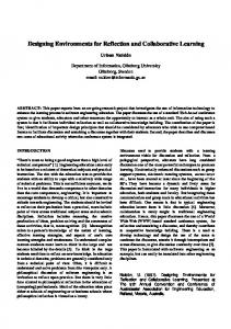
images. Proper seeding of the flow, illumination and camera capture are the basis of this procedure. While system configuration may be difficult, with the correct experimental set-up the acquisition phase is simply a matter of utilizing proper hardware to record the information. After the image acquisition is complete, analyzing the data and extracting the relevant information becomes a matter of digital image processing. Analysis software requires good quality image content in order to achieve accurate results. Two specific problems that may arise are unwanted system vibration and reflection of laser light off the surface of the test model. System vibration is flow induced, and leads to inaccurate displacement values, and therefore to biased velocity values. After an exhaustive literature search, very little information was found that addressed the vibration problem. One possible solution to this problem is the use of an isolated optical research table. However, this is very difficult under most testing situations because of the necessary space requirement. Reflection of the laser light sheet off the surface of the test model can contaminate the PIV images. PIV data processing software is unable to recover information near areas of reflection. There must be a high signal to noise ratio for the software to distinguish accurately between particles and background noise. The reflection issue has been addressed in several experiments. Wang et al11 noted this problem while testing a model of an Apollo type spacecraft. They chose to solve the problem by taking images only behind the model where no reflection was present. This approach captured important information concerning vorticity in this particular experiment. However, in general this approach excluded important data near the model surface. Oshima et al12 approached the reflection problem by painting the model with flat black paint to reduce reflection. The authors made no mention of the success of this attempt. However, it was used in the current research with limited success. Uzol et al13approached the problem by using image enhancement techniques. While using PIV to study turbo-machinery, they obtained images that were saturated with light in regions near the blade area. This resulted in too little contrast in the images, and the particle information was lost if special image enhancement techniques were not used. The series of filters shown in figure 1.3 was developed to correct the reflection problem.

_ Maximum Filter 3x3 Mask

-Median Filter 11x11-21x21 Original Image Mask

Histogram Equalization

+

Figure 1.3: Reflection Removal Model

10

Cross-correlation Analysis

The filter system begins by using the maximum filter to enhance the contrast of the tracer particles. The median filter then removes the particle traces while leaving large objects in the image. Differentiation between the maximum filtered (but not median filtered image) and the median filtered images leave the particle traces while eliminating most of the unwanted parts from the final images. The final step in the image enhancement is the implementation of a histogram equalization program that enhances the particle traces within the image. Image processing is completed by cross-correlation and output of the final vector maps. Uzol et al14 claimed to have greatly reduced the reflection and improved the information recovery in the images. PIV testing was conducted at the NASA Langley Research Center’s Quiet Flow Facility (QFF) during the summer and fall of 2002 to visualize and measure the flow field over the flap side edge region of a high lift model airfoil. As mentioned earlier, unwanted noise was produced by vortices when air from the pressure side of the airfoil escaped around the edge of the flap and combined with the flow on the suction side of the flap. To fully understand the noise generation mechanisms, it was important to visualize the flow very close to the flap model. The airfoil model that was tested is an aluminum NACA 63_2-215 that suffered from a great deal of reflection. Steps were taken to reduce the occurrence of laser reflection from the surface of the test model. These steps included using flat black paint to absorb the incident light, and the use of laser beam blocks to “chop off” the light sheet close to the surface of the model. Although helpful, these techniques did not completely eliminate the occurrence of reflection. Figure 1.4 is an example of an image taken using the beam blocks and black paint.

Flap pressure side

Flap trailing edge

Light sheet

Figure 1.4: Sample Image with Beam Blocking

11

As seen in Figure 1.4, the combination of these techniques proved to be insufficient to completely eliminate reflection. It was determined that image processing software would need to be developed to eliminate the reflection from the PIV images. The QFF is an anechoic wind tunnel facility designed primarily for acoustical testing15. The entire room structure is mounted on springs that isolate it structurally from the remainder of the building and therefore minimize structural noise arising from other parts of the building. As such, the room is essentially subject to rigid body vibration while the tunnel is running. The cameras were mounted as rigidly as possible. However, room vibration and vibration occurring in the camera mounts could not be avoided. Use of an optical table was also ruled out by the structure of the test area as well as by available space limitations. It was decided that the vibration issue would also need to be addressed through software development and implementation. 1.4 Scope and Objectives The objective of this work is to develop a method to eliminate the adverse effects of reflection and vibration in the post-processing of PIV data. The data that were acquired in the QFF “blown flap” experiment will be used to demonstrate the applicability of the method. The image processing techniques and computer codes used to remove the effects of reflection and vibration will be described.

1.5 Organization of paper An explanation of physical and technical principles of PIV is given in chapter 2. In chapter 3, the experimental set-up of the QFF “blown flap” experiment will be explained briefly. In chapter 4 the methodology used in developing the computer codes that eliminate reflection and vibration from the PIV images will be presented in detail. A section will also be included on the operation of the codes. Finally chapter 5 will present the results and conclusions that have been obtained by applying the codes to the postprocessing of PIV images.

12

2. Physical and Technical Background

PIV research can be divided into two basic phases, data acquisition, and image processing and analysis. These phases will be discussed, as will the important aspects of each phase. Data acquisition involves the actual physical components of the PIV system. The discussion will include seeding of the flow, laser illumination of the flow field, and acquisition of the information through the use of digital photography. The image processing section will include all relevant aspects of analyzing the images. Important information including correlation of the images and post processing of the data will also be considered. 2.1 Seeding the Flow PIV research is strongly dependent on good seeding quality in order to obtain quality images for analysis. PIV relies on the assumption that tracer particles will follow the local flow conditions and therefore give an accurate representation of the actual flow properties. The seed must also be of the proper density and be homogeneous throughout the flow. A proper seeding system must be designed for each experiment based upon individual testing conditions. The focus of this section will be the design of seeding systems for gaseous flows in wind tunnel situations. A source of error is the influence of gravitational forces on the flow. If the density of the particles is not comparable to that of the fluid it is not feasible to assume that the particles will accurately represent the fluid motion. Raffel et al16 developed the following equation to estimate velocity lag for a particle in a continuously accelerating flow:

Vlag = Up – U = d p

2

(ρ p − ρ ) 18µ

a

(2.1)

where U is the mean flow velocity, Up is the particle velocity, dp is the particle diameter, a is the acceleration of the fluid, and µ is the dynamic viscosity. If the density of the particle (ρp) is much greater than the density of the fluid (ρ), the step response of Up follows the exponential law   t Up (t) = U 1 − exp τ s 

where the relaxation time τs is given by

13

   

(2.2)

ρp τS = dp 18µ 2

(2.3)

Hence, τs is a good measure of a particle’s ability to attain velocity equilibrium with the fluid. This equation clearly shows that because of the difference in density between the seed particles and the fluid, the particle diameter should be kept as small as possible to ensure good tracking capability. Another requirement that must be addressed is the light scattering properties of the seed particles. If the particles are too small they will not be able to reflect enough light to produce good quality images. It is obvious that a compromise in particle size must be made. PIV testing is possible in both liquid and gaseous flows. Gas flow requirements are much more difficult to satisfy than liquid flows and require more accurate design preparation. The most common particle size used in gas flows is approximately 1-5 µm17. It is now commonly accepted that this size range will meet both of the requirements necessary to produce high quality images in gaseous flows. Seeding is now a matter of finding a non-toxic material that can be distributed homogeneously with the proper particle density in the flow. For many PIV measurements in airflow, Laskin nozzle generators and olive oil are used. The particles generated are advantageous because they are non-toxic, they stay in the air for long periods of time, and they do not change size significantly under varying conditions. Figure 2.1 illustrates the configuration of an aerosol oil-seeding generator.

Pressurized Air (Separate Pipe) Seed particles

Pressurized Air Laskin nozzles

Impactor plate Seed solution

Figure 2.1: Seed Generator Diagram

The generator consists of two separate air inlets and one aerosol outlet. The housing is generally a cylindrical canister with four supply lines extending down into the seed solution. The supply tubes are closed at their lower end and four Laskin nozzles 1 mm in 14

diameter are located in each tube as illustrated in figure 2.2.

Figure2.2: Single Laskin Nozzle Diagram

A horizontal impactor plate is located inside the container so that there is approximately a 2 mm gap between the cylinder housing and the plate. The second pressurized inlet and the aerosol outlet are connected directly to the top. Compressed air with one atmosphere pressure difference with respect to the outlet is released into the Laskin nozzles and creates bubbles in the seed solution. The shear stress that is produced by the Laskin nozzles creates tiny seed droplets within the bubbles. The bubbles then carry the tiny particles to the seed solution surface. The particles rise toward the impactor plate, and large particles are retained while smaller particles are able to reach the aerosol outlet. The number of particles produced can be regulated by the air supply at the nozzle inlets, and the second air supply line into the top of the container controls the particle concentration. The output particles from such a generator are generally considered to have a mean diameter of approximately 1 µm, which is an optimum diameter for seeding airflows. The proper placement of the seed generating system in the wind tunnel must now be taken into consideration. This aspect is very important to ensure proper density of seed, such that the distribution in the flow is homogeneous throughout the test section. Certain factors must be considered to assure the highest quality results. The first of these is that the seed may be dangerous to the experimenter’s health. While in general most seed 15

material used is non-toxic, prolonged exposure is usually an inhalation hazard. Also some materials may be highly evaporative, and must be injected close to the test sections for this reason. The injection must be done in such a way that it will not disturb the flow conditions. Many wind tunnels are designed to reduce turbulence, and the seed may need to be supplied from a large number of inlets to assure proper mixing of the material. With advance consideration of the test facility, the researcher can meet all requirements necessary to capture high quality images. 2.2 Laser Illumination Illumination of the flow field is the next major consideration in the design of a high quality PIV system. Many types of lasers are commercially available in today’s technology. These include helium-neon lasers, argon-ion lasers, and neodym yttriumaluminum-garnet (Nd-YAG) lasers. Of the three types the latter is by far the most important and widely used in PIV research. Nd-YAG lasers emit only the strongest wavelength (λ) 1064 nm. By including a quality switch (Q-Switch) in the laser, it may be operated in a triggered mode. The Q-switch timing affects the resonance characteristics of the optical cavity, and if the Q-switch allows the resonance to occur at the highest energy level it produces a maximal-energy output. By operating the laser in double oscillating mode the user is able to control the separation time independently of the pulse strength. Nd-YAG lasers use second harmonic crystals to double the frequency of the emitted light. This allows the 1064 nm infrared light to be emitted as 532 nm visible green light. After the frequency doubling approximately one third of the original energy is available at the 532 nm wavelength. The energy emitted by this type of laser is generally in the range of 100-500 mj per pulse. Pulse separation times using state of the art technology can be as low as 1 µs. 2.3 Light Sheet Optics The small diameter laser beam emitted by the Nd-YAG lasers must subsequently be transformed into the laser light sheet necessary to record PIV images. This is done through use of light sheet optics. When using Nd-YAG lasers a cylindrical lens is the essential component in transforming the emitted light. Because of the properties of the Nd-YAG laser, it is also necessary to use a combination of different lenses to achieve a very thin light sheet of high intensity. Many researchers find that a combination of a cylindrical lens and two spherical lenses makes the PIV system more versatile. An example of such a system is shown in figure 2.3

16

Side View

Light Sheet

Spherical Lens

Spherical Lens

Cylindrical Lens

Thickness

Top View

Figure 2.3: Light Sheet Optics Diagram

In general, the use of both spherical and cylindrical lenses does not allow the height and thickness of the light sheet to be manipulated independently. If the optics system is configured as shown in figure 2.3 it is possible to control both height and thickness of the light sheet independently. The height can be adjusted by changing the focal length of the cylindrical lens. This height will vary depending on the application of the system and will need to be as versatile as possible. The thickness of the light sheet is also readily adjustable; this is accomplished by changing the distance between the two spherical lenses. The configuration of the optics is critical in optimizing the light sheet intensity. Because the light sheet intensity distribution is so important for quality of measurement, especially in the out of plane direction, it is important to configure the optics system correctly to produce the desired experimental results. The last optical consideration is that the experimenter must avoid reflection among the components. Uncoated lenses in air exhibit a small reflectivity, generally on the order of 4 percent. This reflection is usually acceptable unless it is focused on other components of the optics system. It is generally recommended that the reflection from the lenses be focused so that it is not reflected 180° from the incoming light. The reflected light can cause damage to expensive equipment such as the actual lasers, and the CCD cameras that will be described in the next section. 2.4 Digital Image Recording and Storage Early PIV research relied on standard photographic techniques and subsequent 17

digitization of the information after the acquisition phase. With the recent advances in electronic imaging, PIV now makes use of state of the art CCD cameras. A major advantage of digital imaging is that information, and therefore feedback, is immediately available to the experimenter during the recording phase. This is a tremendous advantage in time and cost to the researcher because mistakes in the data can be corrected before the time-consuming analysis procedure begins. CCD cameras and their application will be the focus of the current section. CCD cameras convert light into electronic charge. A CCD camera is actually an array of many CCD sensors called picture elements, or pixels. The size of a pixel is generally around 10x10 µm16 and digital cameras that are used for PIV usually contain an array of 1-3 million pixels depending on the image size. As anyone familiar with digital photography is aware, these numbers, or resolutions, are increasing at a very rapid pace. Pixels operate by converting light into electronic charge and storing the charge. The configuration of an individual pixel is shown in figure 2.4.

Metal Conductors Incoming Light Oxide Layer

e- e- e-

n - layer e-

p-layer

Figure 2.4: Individual Pixel Diagram

Pixels are composed of a silicone semi-conductor layer with metal conductors at the surface. Below this is an insulating oxide layer, an n-layer (anode), and the p-layer (cathode). When a voltage is applied between the metal conductor and the p-layer an electric field is generated in the semi-conductor. The minimum in this electric field is termed a potential well, and is caused by lack of electrons below the center of the pixel. The potential well serves as a capacitor allowing the pixel to store electrons. When light within a set bandwidth hits the pixel and enters the p-n junction an electron hole pair is formed. This hole carries a positive charge and is absorbed in the p-layer of the pixel. The free electron that is generated in this process moves toward the potential well where it is stored. Electrons continue to accumulate in the well as long as the exposure to light continues or the limited capacity of the potential well is exceeded. Potential wells have a capacity of between 10,000 and 100,000 electrons. When the well saturation capacity is 18

exceeded the electrons begin spilling into the neighboring pixels. This is known as bleeding and will lead to overexposed white areas in the image. The newest CCD technology has accounted for this problem by incorporating conductors to catch the excess electrons before they are able to migrate to the neighboring pixels. Figure 2.5 shows a PIV image where bleeding has occurred.

Y

Figure 2.5: Potential Well Saturation X

When the exposure is complete the information from the pixel array is read into storage pixels. The information storage methods and capabilities vary among different types of CCD cameras. The most versatile type of CCD used in PIV research at this time is the full frame interline transfer CCD (FFCCD). It is the most advanced technology available and will be used to explain image transfer and storage in the following discussion. The electronic information storage system is made up of four major components. In an interline CCD camera each pixel has its own storage site located between the active pixels. The active pixels make up the photo diode array, and the storage pixels are termed the CCD array18. The remaining components of the storage system are a frame grabber board, and the actual computer hardware. When images are taken at a high frame rate, typically 30 frames per second, information from each image must be exchanged very rapidly in order to accommodate the next incoming image. When images are exchanged this quickly they can develop a high level of read-out noise. This will greatly reduce the quality of the images and must be avoided at all costs. This problem has been solved by use of the frame grabber board, which essentially stores massive amounts of information and feeds it at a much slower rate to computer hardware. Using multiple frame single exposure PIV as an example the acquisition phase will now be briefly summarized.

19

The images are taken by the active pixels, or photo diode array, and are quickly moved for storage into the CCD array. A method called frame straddling is used to accommodate this process. Frame straddling synchronizes the laser pulses with the camera frame rate so that all the information moves through the system properly. The first laser pulse and acquisition by the active pixels obviously occur at the same time. The information is transferred to the CCD array before the second pulse occurs. When the second pulse occurs the information is again acquired by the active pixels, but the previous information moves from the CCD array through a charge to voltage converter to the frame grabber board that stores the information. Each pixel in the array now has a separate voltage value assigned to it. The computer will eventually read these voltages as grayscale values. This process repeats itself until all of the images in the series have been recorded. The images must now be read slowly from the frame grabber so that the read-out noise level can be kept as low as possible. When all images have been read into the computer hardware the actual PIV processing can begin. 2.5 Image Evaluation Methods All PIV techniques require some sort of interrogation scheme to extract the displacement information. Earlier PIV methods used low particle density visual tracking methods to locate individual particles in successive images. A higher density of seed particles is required in order to obtain larger PIV vector maps, especially when comparing PIV data to numerical calculations19. PIV in its present form is considered to be a medium particle density method. The medium density assignment is characterized by the fact that matching pairs of particles cannot be visually detected in successive images. Therefore statistical methods are used to analyze the images. The main objective of PIV evaluation is to determine the displacement between two grayscale particle images. PIV software breaks the large image arrays into smaller regions, generally 32x32 pixels, called interrogation regions. Analyzing these smaller regions statistically it is possible to match particles, or groups of particles, between successive image pairs. The processing can be thought of as the linear system shown in figure 2.6 Input Image (Image 1)

Transfer Function (Displacement)

Output Image (Image 2)

Noise Addition

Figure 2.6: Linear System Signal Processing Model

With both the input and output images known, and the fact that the background noise and 20

displacement provide no information about each other, it is necessary to estimate the displacement statistically using the information from the interrogation regions as random samples20. The discrete cross-correlation function

R12 ( x, y ) =

K

L

i=− K

j =− L

∑ ∑ I (i, j ) I 1

2

(i + x, j + y )

(2.4)

is calculated over the interrogation region, where I1 represents the intensity values in the first image, and I2 represents the intensity values in a larger region of the second image. Using I1 as a template, it is linearly shifted throughout the interrogation region I2 and produces one cross-correlation value R12 (x, y) for each sample shift (x, y). Using a range of shift values for x and y, a correlation plane is produced. For shift values where particles align with each other the sum of the products of the intensity values will be much larger than elsewhere and will produce a high correlation peak at that point. The highest value in the correlation plane is then used to estimate the particle displacement. Standard cross-correlation is the method used by many PIV software systems. However, it requires an extensive computational effort, on the order of millions of operations16. Recently, software has been developed that uses a much more efficient procedure. Frequency domain correlation and Fourier transforms can be used to more efficiently calculate the cross-correlation of two successive images. Using the correlation theorem that states that the cross-correlation of two functions is equal to the complex conjugate product of their Fourier transforms21 ^

^

R12 = I 1 ⋅ I 2

(2.5)

computational time can be greatly decreased. Here Î1and Î2 are the Fourier transforms of the image intensity values I1 and I2. Using this method it is possible to reduce the crosscorrelation calculations to the system summarized in figure 2.7. Interrogation Regions

Image 1

Image 2

Real to Complex FFT

Complex Conjugate Product

Real to Complex FFT

Figure 2.7: Frequency Domain Cross-correlation

21

Complex to Real Inverse FFT

Output Correlation Data

The Fourier transforms are actually performed using fast Fourier transform techniques (FFT) that reduce the computation time from order [N2] to order [Nlog2 N], where N is the number of computations21. Using this system the computations are reduced to performing two FFT’s, followed by a complex conjugate multiplication, then taking the inverse Fourier transform. The output of the system is a correlation plane of the same size as the original interrogation region. This method is being widely used in state of the art PIV software. Other developments to further increase the efficiency of software are being investigated and implemented continuously. One of the most important aspects of PIV evaluation is finding the position of the correlation peak. The peak can be located to sub-pixel accuracy; estimation accuracy as low as .05 pixels is achievable using 8-bit digital imaging. Using a three-point estimator method, displacement can be determined to ± .5 pixel accuracy. A method which can be used to detect a correlation peak and find the corresponding displacement estimate is to scan the correlation plane to locate the highest correlation peaks R(i, j), and determine its integer coordinates (i, j). Next find the four adjoining correlation values: R (i-1, j), R (i+1,j), R (i, j-1), R (i, j+1). The third step is to apply a three-point Gaussian curve estimator. The following equations are used to determine the displacement from a correlation peak at the subpixel level:

 − ( x0 − x ) 2  f ( x) = C exp   k  

(2.6)

where x0 = i +

ln R( i −1, j ) − ln R( i +1, j ) 2 ln R(i −1, j ) − 4 ln R(i , j ) + 2 ln R(i +1, j )

(2.7)

and y0 = j +

ln R(i , j −1) − ln R( i , j +1) 2 ln R( i , j −1) − 4 ln R( i , j ) + 2 ln R(i, j + 1)

(2.8)

With the recording and evaluation procedures complete, it is now necessary to develop a method to validate and further process the PIV information.

2.6 Data Post Processing

Post-processing of PIV data consists of several aspects. These include data validation, data reduction, and analysis of the information. The first two aspects are accounted for within the PIV software, and will be the focus of this discussion. The PIV data acquired in the QFF blown flap experiment was used to develop new techniques that increase the 22

accuracy of post-processing and these techniques will be presented in following chapters. Data validation is the most critical aspect of post processing. After automated processing of the data, PIV software displays the velocity field vector maps for the user’s inspection. The researcher can examine the resulting vector maps visually and locate certain obviously incorrect velocity vectors22. The incorrect vectors are called outliers and they generally have two distinguishing characteristics. First the magnitude and or direction will be considerably different from the neighboring vectors, and the second characteristic is their location in the field. Outliers can usually be found close to the model surface, or at the edge of the illumination area. The outlier vectors are a result of correlation peaks that were detected that resulted from noise in the image, and not from particle matching. It is essential to detect and eliminate all erroneous data before performing further data processing. In particular, processing involving differential operators will be smeared as a result of these outliers, and quality data will be lost as a result. In earlier PIV research it was possible to remove these outlier vectors interactively. As a result of the quantity of data generated with state of the art PIV systems, algorithms must be implemented that will automatically detect these outliers and eliminate them from the final data. Although there is not a general solution for data validation, two methods are commonly being used at the present time. In describing the global histogram23 and dynamic mean value operators for data validation, the mesh system used by PIV software must first be addressed. When using PIV software the experimenter must define a mesh system within the image being analyzed. Usually rectangular in shape, newer software packages make provisions to custom fit meshes to user defined shapes. A 3 x 3 section of a rectangular mesh is shown in figure 2.8.

•Y

Y (v)

U (i-1,j+1)

U (i,j+1)

U (i+1,j+1)

U (i-1,j)

U (x,y)

U (i+1,j)

U (i-1,j-1)

U (i,j-1)

U (i+1,j-1)

X (u) •X

Figure 2.8: PIV Mesh System

The velocity vectors U(i, j) are an example of a typical flow field; nine points are 23

contained in the mesh of figure 2.8. The mesh will be used to describe the two data validation methods listed above. The global histogram operator uses the principle that the difference in magnitude of the vector being investigated (U (x, y)), the central vector, and the neighboring vectors will be below a certain threshold value ε. U difference = U ( i , j ) − U ( x , y ) ≤ ε

(2.9)

Equation 2.8 is considered to be valid as long as the length scale of the fluid flow is much larger than the distance between neighboring vectors. Therefore all correct data must lie within in a certain area in the (u, v) plane. The global histogram operator sets upper and lower limits of the neighboring vector ± ε, the limits of possible flow velocities. The vector is rejected if it fails to meet the criteria. The velocity plane is divided into small cells so that a velocity histogram can be calculated. A rectangle is placed around the area with the highest number of velocity vectors present. The velocity vectors in each cell are then checked individually and the vectors outside of this region are labeled and rejected. Using this method, the researcher is able to reject vectors, as well as to determine the number of rejected vectors, gaining additional information about the quality of data. The limitations of the global histogram operator are that it does not account for the direction of the vector, and that it fails in the presence of strong velocity gradients such as shocks in transonic flows. With this in mind most software utilizes both the global histogram and the dynamic mean value operator. The dynamic mean value operator checks each velocity vector individually with the average value of its neighboring vectors: 1 N (2.10) ∑U (i, j)(n) N n=1 The averaged magnitude of the vector difference between the average vector and its neighbors is also found using MeanU (i, j ) =

1 σ U= N 2

N

∑ (Mean

U

(i, j ) − U (i, j )(n)) 2

(2.11)

n =1

A 3 x 3 mesh (N=8) is standard for this procedure although larger sizes are also utilized in some software. A vector will be rejected when

MeanU (i, j ) − U ( x, y ) ≥ ε

(2.12)

This test also has the important characteristic that it can be modified for use on the u and v components of the vector; this modification takes into account the direction of the vector as well as its magnitude. The problem with velocity gradients is also accounted for by modifying the threshold, ε, locally in areas where large gradients are present. 24

Satisfactory data have been obtained at the edge of the flow field where N is less than eight by adding lines and rows to the edges and filling these with the mean value for the entire flow field16. By using both algorithms it is possible to reject all incorrect outlier vectors and therefore satisfactorily validate the raw PIV data. After validating the data it is possible to replace the deleted vectors using bilinear interpolation. Westerweel22 stated that the probability of having another incorrect vector in the same neighborhood as the deleted vector is represented by a binomial distribution. Therefore data can be obtained from the valid neighboring vectors. The rest of the missing data can be obtained using a weighted average of the surrounding data as suggested by Agui et al24. Experimental data may be affected by noise whereas numerical data will not be. Therefore, smoothing of the data may also be necessary. This is accomplished by using a convolution of the data with a 2x2 or larger kernel with equal weights. If the kernel size is kept below the interrogation window size further filtering of the data can be kept to a minimum. The velocity information may not be as important as some derivative or integral information that can be calculated using the software. Because PIV cannot generate information about the pressure and density fields, the velocity information alone cannot recover all terms in the Navier-Stokes equation25 ~ DU ~ ~ ρ = −∇p + µ∇ 2U + F Dt

(2.13)

where F represents body forces such as gravity, and are normally neglected. The vorticity field

ω~ = ∇ × u~

(2.14)

may be of much more significance than the velocity field itself. Assuming incompressible ~ flow where ∇ ⋅ U = 0 , the Navier-Stokes equation can be written in terms of the vorticity in the form ∂ω~ ~ ~ + U ⋅ ∇ω = ω ⋅ ∇U + ν∇ 2ω~ ∂t

(2.15)

Standard PIV is a planar technique and is only capable of providing data that can be differentiated in the x and y directions. Therefore only the following terms of the deformation tensor can be recovered by 2-D PIV:  ∂v ∂u  −   ∂x ∂y 

(2.16)

 ∂u ∂v  −   ∂y ∂x 

(2.17)

ω z = 1 / 2

ε xy = 1 / 2

25

η = ε xx + ε yy =

∂u ∂v + ∂x ∂y

(2.18)

The first equation is the out of plane vorticity component, the second is the in-plane shearing, and the third term is the in-plane extensional strains. 2-D PIV must use a finite difference scheme in order to obtain the terms of the deformation tensor (equation 2.19 below). This procedure leads to error propagation in the derivatives of the velocity estimates. 2D-3C PIV ( explained previously) was the method used in the QFF testing. By using vectoral techniques 2D-3C PIV is capable of producing all nine terms of the deformation tensor16

∇ u~ =

 ∂u  ∂x  ∂u   ∂y  ∂u   ∂z

∂v ∂x ∂v ∂y ∂v ∂z

∂w  ∂x  ∂ w  ∂y  ∂w   ∂z 

(2.19) Hence the error is much less than found using the finite difference schemes. It should be noted that the additional information of w, the third velocity component, does not produce any additional information regarding the vorticity or strain.

26

3. Experimental Set-up

The following section will describe the testing that was performed in the QFF facility. The experimental set-up will be described first, followed by a description of the equipment that was used in testing. 3.1 The Experiment The objective of the experiment was to visualize and map the flow field near the side edge of a flap model. 2D-3C PIV was used to obtain all three components of the velocity vector. In the test, high pressure air is blown through a slot that is located along the flap side edge. PIV measurements were taken for the four flap configurations shown in figure 3.1.

Figure 3.1: Blown Flap Edges

The impact that each blown flap configuration was found to have on the structure of the flow is beyond the scope of this work. Only specifics and results pertaining to the PIV

27

data acquisition and processing will be discussed. A detailed description of the blown flap PIV experiment and of the results obtained is given in reference 30. The test was conducted at a mean flow speed of Mach number (M)= 0.17, and three different Mach numbers for the air exiting the flap slot were considered. PIV measurements were taken with the light sheet located in a plane perpendicular to the flap chord. A diagram of the different measurement locations is presented in figure 3.2.

Figure 3.2: Light Sheet Locations in Images

The light sheet was positioned approximately between the point where the vortex moves from the pressure side to the suction side of the flap (Cut F) and slightly past the trailing edge (Cut A). By selecting these viewing locations it was possible to clearly visualize the flow field in the area of interest. The flow field was illuminated by the two laser systems shown in figure 3.3. The light sheet was aligned to illuminate flow in all areas near the flap side edge. It was positioned parallel to the flap trailing edge and normal to the flap chord as shown on the left hand side of figure 3.3. Each laser was capable of illuminating the entire area of interest. However the reflection from the model made it impossible to capture the flow field in one view. This made it necessary to record the flow field in three separate parts. The model reflection had to be masked so that information could be obtained near the flap surface. The first part used the side laser to record the information above the flap model, using beam blocking techniques to mask the reflection within and below the model plane. The second acquisition also used the side laser, and blocked the field of view above and within the model plane. The third part was obtained using the pressure side laser, where model reflection was not an issue, to obtain the flow field information within the plane of the model.

28

•

Two laser systems – Side laser – (No information in flap side area)

1

–

2

Flap

Pressure side laser (Used to record missing information)

Trailing edge

3

Figure 3.3: Light Sheet Configurations

Two cameras were used to record the images in the stereoscopic configuration. The camera locations were influenced by space limitations and field of view considerations. The depth of field issue in the images would also prove to be a determining factor in camera placement26. The camera configuration is shown in figure 3.4

Camera A

Camera B

Figure 3.4: Camera Configurations

29

The accurate positioning of the cameras made it possible to record the images near the model edge. An example of the recorded images and the combined viewing area is presented in figure 3.5.

Fiduciary Marks

Camera A

Camera B

Y

Flap Trailing edge X

Pressure side

Figure 3.5: Sample Image and Viewing Area with No Lasers

The figure shows the two camera views that were used throughout the test. The area in blue shows the combined viewing area that is made possible by the laser positioning described previously. Using the three part system to record the flow field reduced the reflection problem from nearly impossible to manageable. Post processing of the images was required to eliminate the remaining reflection prior to the final velocity vector processing. The fiduciary marks shown in the figure were used to eliminate system vibration, and this procedure is described subsequently. 3.2 Experimental Facility PIV testing that mapped the flow field near the flap side edge region of a NACA 63_2215 airfoil was conducted in the NASA Langley Research Center QFF facility in 2002. The QFF is an anechoic open jet facility. The flow circuit is equipped with turbulence screens, baffles, and turning vanes to ensure that the flow at the test section is very quiet and low on turbulence. Figure 3.6 is a schematic of the flow circuit.

30

Figure 3.6: QFF Diagram

Low-pressure air is fed from a blower house located outside of the actual building. The blower house contains the low-pressure fan used to generate the flow. The air enters a duct system that utilizes acoustic splitters and turning vanes that assure quiet low turbulence flow. As the air enters the building it is turned 90˚ from horizontal to vertical before entering the nozzle and then the test section. The test section is located inside an anechoic chamber; it is a two-foot by three-foot open jet test section. Two vertical side plates are attached to the short sides of the nozzle. These side plates are approximately six feet high and are used to support the test model above the nozzle exit. The air exits the building by means of a larger cross-sectional area eductor system. The entire structure of the anechoic chamber is isolated from the rest of the building by springs that minimize the structure borne noise arising from other parts of the building15. The QFF has been in operation at Langley since 1973 and has been used for a wide variety of testing applications. It was originally designated for acoustic testing but was later equipped for PIV testing in 1999.

31

3.3 Test Equipment The equipment that was utilized for the QFF experiment is described in this section. Beginning with a description of the flow seeding process, all aspects of the experiment will be discussed, including some aspects that are specific to this test and were not mentioned in the basic theory section.

3.3.1 Flow Seeding The seed used for the testing was C26H50O4 or Bis (2ethylhexyl) sebacate, 90%. It was chosen because it possessed certain desirable characteristics. It has a particle size of 1 µm, which satisfies both the light scattering and density requirements necessary to produce quality images. It is also non-toxic, and highly evaporative, so it is a cleaner application than oil based seed materials. This particular seed had also been used successfully in previous PIV testing26. Seed particles were introduced into the flow upstream of the low-pressure air fan by means of two Laskin nozzle aerosol generators. A seed generator is shown in figure 3.7, and it is the type described in section 2.1.

Figure 3.7: Aerosol Seeding Generators

The seeding system in the QFF was capable of providing proper seed density, homogeneous distribution of seed particles, and the correct particle diameter. The generation and distribution process could be controlled remotely from the QFF control room.

32

3.3.2 Nd:YAG Lasers The laser illumination used in the QFF was provided by two New Wave Research, Inc. Gemini PIV Nd: YAG lasers, shown in figure 3.8.

Figure 3.8: QFF Nd: YAG lasers

The Gemini lasers operated at a wavelength of 532 nm, providing approximately 120 mj of energy per pulse. The laser was a two-cavity laser that operated at a maximum pulse rate of 30 Hz, or 15 Hz for each laser cavity. (Two-cavity lasers were basically two lasers that alternate pulses combined in one unit.) The laser used a closed loop water-cooling system. Deionized water was circulated between a water to air heat exchanger and the laser head to maintain proper temperature of the laser head. The laser could be either internally triggered or controlled externally by a computer that synchronized the pulses with the cameras. The QFF PIV system operated in the externally triggered mode. The Gemini laser produced a 5mm diameter laser beam that is very stable and could be adjusted to produce the light sheet used in recording the PIV images. 3.3.3 Light Sheet Optics The optical configuration used to produce the light sheet was the same as shown previously in figure 2.3. The first spherical lens had a –200 mm focal length. This caused the 5mm diameter incoming laser beam to expand slightly between the first and second lens. The second spherical lens had a 200 mm focal length. Adjusting the distance 33

between the two spherical lenses set the beam thickness. The QFF experiment required a light sheet thickness of approximately 1mm. The light then passed through the cylindrical lens where it formed the light sheet. Two different cylindrical lenses were used for the two laser configurations that were previously described. The focal lengths were -40mm for the pressure side laser, and –50mm for the side laser configuration. The different lenses produced light sheet heights of approximately 12mm and 15mm, respectively. 3.3.4 CCD Cameras and Frame Grabbers The cameras that were used were Redlake (formerly KODAK) MegaPlus ES 1.0 crosscorrelation CCD cameras with Nikon 105 mm lenses. Using the external trigger mode the frame rate (30 Hz) was synchronized with the laser pulse rate. The cameras were operated using multiple frame single exposure PIV mode. This particular camera is a full frame interline transfer CCD that records images with 1008 pixels horizontally (x), and 1012 pixels in the vertical dimension (y). The actual pixel size is 9 x 9 microns. The cameras required special mounts that were very rigid to minimize the effects of vibration because of wind tunnel operation (figure 3.9).

CCD Camera

Rigid Camera Mount Lens

Figure 3.9: Rigid Camera Mounts

These mounts, while effective in reducing vibration, proved to only partially eliminate the problem, and further steps were needed to completely eliminate the vibration. Coupling the cameras with a National Instruments IMAQ frame grabber, the system was able to achieve sub microsecond frame straddling and low read-out noise levels.

34

3.3.5 PIV Processing Software NASA obtained the entire QFF PIV system from Integrated Design Tools27 (IDT) in 1999. The package is integrated so that all components worked together correctly. IDT Provision software was used to do the actual vector processing. In the 2C-3D mode the software combined the images that were obtained separately from both cameras into one 2016 x 1008 pixels image, with one camera view on the left and the other on the right side of the new images. The software then compared images sequentially (1 to 2, 3 to 4 and so on) using cross-correlation techniques. “Tecplot” software was then used to plot the velocity vector results. Adjustments could be made so that the IDT software would also compute and plot derivative quantities. A sample velocity vector map is shown in figure 3.10.

Figure 3.10: IDT Velocity Vector Map

The raw velocity vector data were also stored in Tecplot files, so that the researcher would have convenient access to the information for further post processing. User interaction with the IDT software in the post-processing phase yielded the velocity or derivative information depending on the desired results.

35

4. Vibration and Reflection Removal Algorithm In order for a PIV system to produce information near a model surface, the reflected laser light from the surface must be removed. This process is absolutely necessary in many test situations because the desired information is located very close to the model. Correlation methods, and therefore output data, cannot be considered to be reliable if too much noise is present in the images because of the possibility of false correlation peaks. The effects of system vibration also cause bias errors in PIV testing. System vibration consists of model and camera vibration and causes incorrect displacement values to be processed by the software, yielding biased results. In the course of the QFF experiment, algorithms were developed to address both the reflection and vibration problems. With a series of computer codes it is possible to eliminate these unwanted effects from PIV results. The algorithms were developed using “Matlab” software and can be adapted to any PIV test situation. Sample algorithms are presented in Appendix 1. The following discussion presents the algorithms and explains the methodology behind their development and their application to the QFF testing. The algorithms remove the effects of reflection and vibration from PIV images. The two issues, while resolved in the same computer code, must be explained separately due to differing methodology. The reflection issue is the simpler of the two methods and will be explained first. 4.1 Reflection Removal PIV images consist of three main components, reflections from seed particles, background, and background noise (reflection). A sample 2016 x 1012 pixel image is presented in figure 4.1. The three components are clearly visible in the figure.

Figure 4.1: Sample Image Prior to Processing

36

A high quality PIV image will have high contrast between particles and background with no reflection or other background noise present. The images are recorded as grayscale images containing values of 0 to 255 for each pixel. Zero in this case corresponds to black, or no light, with 255 being the maximum value, or white. In the best quality image all pixels would be either 0 or 255, with complete contrast and no possible correlation between the particles and background. The algorithm that has been developed in this research has attained this degree of contrast or signal to noise ratio (SNR). This is accomplished through the series of filters and enhancing adjustments that will be described below. Post processing begins by accessing the set of images that are to be processed; in this case these images were originally recorded in acquisition groups of 60 images. The images were later regrouped with each acquisition set containing 420 images. This regrouping made the processing much more automated. It was also the maximum number of images that the IDT software could process in each group. For simplicity the first image in each acquisition set was used as a reference image and enhancements were performed on the image. The images were cropped into two images, each containing 1008 x1012 pixels, or the separate camera views. This step in the procedure was very important because each camera captured different amounts of light and therefore required separate enhancement settings. After the image was cropped, the separate enhancement settings were used throughout the program for each camera view. A high pass filter is applied that effectively removes all particles from the image. By applying this filter (called a “structural element filter28”) of a specified pixel size, all elements in the image below this threshold are removed and larger objects are retained. In the QFF testing the structural element was a disc shape ranging from 2 to 5 pixels in diameter depending on the specific image. The second step in processing was the enhancement of the reference image. Matlab contains a filtering function (Imadjust) that uses the grayscale values in the pixel information and converts the image to a binary image. While not a true binary image, with pixel values of 0 for black and 1 for white, the values of 0 and 255 served the same purpose. The function asked the programmer to set a threshold as a percentage of the 0 to 255 pixel range. The threshold was then applied and any pixel below, say, 50% or a value of 128, was designated as black or 0. Any value above 128 was set to 255 and designated as white. This threshold could be set to any percentage value between 1 and 100 % depending on the quality of the image that was being processed. A typical value in the QFF testing ranged between 65 and 80 percent. The image of figure 3.11 is shown after enhancement techniques were applied, in figure 4.2.

37

Figure 4.2: Reference Image After Filtering and Enhancement

Figure 4.2 shows an enhanced reference image that was used to remove reflection from post processing. The seed particles were removed with the “structural element filter”, and the reflection from the flap side edge and fiduciary marks was enhanced to provide maximum contrast in the image. The reference image was used in both the vibration and reflection sections of the code. However, the images were used differently in each case. Because of this it was necessary to implement two separate enhancement sections in the code. When concerned with reflection removal, the input values were set to achieve the maximum contrast and reflection enhancement. Figure 4.2 is an example of reflection enhancement. After the reference image was enhanced, the algorithm subtracted the reference image from each image in the acquisition set on a pixel by pixel basis removing the reflection. Each resulting image was therefore a grayscale image, and required another enhancement step. This step used the same function described above, but utilized different enhancement settings to achieve the highest signal to noise ratio in the output image. A sample output image is shown in figure 4.3.

38

Original Image with Background Noise

Subtract Enhanced Image

Output Image without Background Noise

To IDT software

Figure 4.3 Final Output Image from Algorithm

The image of figure 4.3 is clearly a high quality PIV image. All particles have a value of 255, and the background has a 0 value. Cross-correlation techniques had no difficulty with false correlation peaks due to noise when using these processed images. The output images had the surface reflection removed; they also were adjusted for vibration, and this will be the subject of the following discussion. 4.2 Vibration Correction and Image Shifting The effects of vibration are more difficult to address. While reflection issues could be resolved using one algorithm, vibration removal required the use of four separate algorithms. A flow chart of the algorithm organization is presented in figure 4.4 and a brief description of the algorithms will now be given.

39

Background Images

Acquisition Background

Acquisition Code 1

Acquisition Code 2

Acquisition Origin

IDT software

Raw Images

Figure 4.4: Algorithm Flow Chart

• • • •

Acquisition code 1 shifts the fiduciary mark centroid to the centroid location of the same fiduciary mark in a reference image. Acquisition code 2 determines the pixel coordinates of the fiduciary mark centroid in the reference image set. Acquisition background code finds the centroid pixel coordinates of the same fiduciary mark in background images that were recorded under no flow conditions. Acquisition origin code shifts the fiduciary mark centroids of all images in a set to the location of the background image fiduciary mark centroid.

The first algorithm, Code 1, used fiduciary marks, illustrated in figure 4.5, that were painted on the surface of the flap model as reference points in the images.

Figure 4.5: Background Image with Fiduciary Marks

40

In order to remove the effects of vibration it was necessary to locate the centroid of a single fiduciary mark in all of the images contained in the acquisition set. Beginning with the reference image, a series of adjustments must take place in order to accomplish this task. In order to fully explain the algorithm, a 1008 x1012 pixel, high reflection, low contrast image will be used throughout the discussion. The image shown in figure 4.6 will be used to illustrate the methodology used in the processing, as well as to familiarize the reader with problems that were encountered during the vibration removal operations of the code. Figure 4.6 was adjusted slightly to darken the image for presentation in this paper.

Figure 4.6 Low Quality PIV Image (Single Camera View)

Images such as this were very difficult to process because no fiduciary marks were visible due to the low contrast and reflection in the image. It was also impossible to process this image using the IDT software without enhancing the image. The enhancement was performed using the image enhancement functions described previously. The resulting filtered image is shown in figure 4.7.

41

Figure 4.7: Enhanced Image with Fiduciary Mark Location

It is clear that this image can be used to locate the fiduciary mark. However, it cannot be used for the reflection subtraction process because it would not remove all of the reflection from the image. Therefore the two enhancement procedures (vibration and reflection removal) had to be performed separately in order to obtain optimum results. The vibration enhancement procedure focused on adjusting the image so that fiduciary marks could be located, while the reflection removal procedure adjusted the image for maximum contrast. Performing both reflection and vibration removal in one algorithm proved to be a very difficult undertaking. The image in figure 4.6 represented the most difficult image to process that was encountered and serves as an excellent example of the versatility of the algorithm. With the reference image enhanced, and the fiduciary mark now detectable, the centroid of the fiduciary mark could be located so that it could be compared with the same mark in the other images of the acquisition set. This was accomplished by cropping the image with a bounding box (figure 4.7), typically 50 x 50 pixels in size. The bounding box was placed around the mark in question and hence a smaller interrogation image was formed. Figure 4.8 was enlarged for clarity; its actual size is 50 x 50 pixels.

42

Enlarged Fiduciary Mark

Figure 4.8: Exploded Bounding Box

This bounding box was then scanned for objects within a certain size range. The x and y centroidal values as well as the area (in pixels) of the objects that were found within the cropped image were stored internally. The size range eliminated all objects that fell outside of the set thresholds. This effectively eliminates any particles or larger objects from processing. The object with the largest pixel area in the bounding box was used for the centroid calculation. The remaining images in the acquisition set were then processed. The algorithm used the centroid location determined from the reference image, and placed a bounding box around that location in each of the images in the acquisition set. Each image was then scanned for objects located within the bounding box as described previously. The centroids of the fiduciary marks in each image were then recorded internally. Calculating the displacement between the reference image and the individual images was then a simple matter of subtracting the x and y centroidal values. Each image must then be shifted by the displacement values so that the fiduciary mark centroids were in the same location as the reference image fiduciary mark centroid. This was accomplished by expanding each 1008 x 1012 image array with additional rows of zero values. Ten rows or ten columns were added to each side of the image to expand the images. This essentially creates a black frame around the original images so that they could be shifted in any direction that was necessary. Figure 4.9 shows the image with the frame placed around it.

43

Figure 4.9: 1028 x 1032 Pixel Image With Shifting Frame

The frame was necessary so that no particle information was lost during the shifting process. Images were shifted by the x and y displacement values that were calculated previously. Cropping the image to the original 1008 x 1012 size, and combining the camera views into 2016 x 1012 images was then performed. This completes the processing through the first code; each images’ fiduciary mark has been shifted to the same pixel location as found in the reference image. The remaining algorithms were designed to locate the centroids of fiduciary marks in the acquisition and background images. The background images were recorded under no flow conditions, and it was assumed that no vibration effects were present in these images. Because the acquisition images had been shifted, it was possible to work only with the reference image in the second acquisition code. There was only one background image and therefore a similar code was used for background processing. The images were then shifted again to the background reference frame and the Matlab processing was complete. In order to accomplish this shifting it is first necessary to explain an important feature of the PIV software. Because of the camera position angles in 2D-3C PIV, the images are essentially stretched or warped when they are recorded29. Figure 4.10 illustrates this phenomenon.

44

Calibration plane

Captured images

Figure 4.10: Image Warping

The distortion of the images in the separate camera views was caused by the fact that the magnification factor was no longer constant across the field of view. This requires an additional means of calibration. The calibration procedure placed a grid within the light sheet location so that the distortion between camera views could be calculated. Algorithms were used in the PIV software that were capable of mapping a distorted foursided polygon to a rectangle. The algorithms generally implement non-linear least squares approaches. Using calibration information and de-warping techniques IDT software could transform the fiduciary mark locations from the image plane to the calibration plane coordinates. The origin location was then located at exactly the same point in each camera view. When comparing the acquisition images and the background image for each cut it was essential that the fiduciary marks that were used were located in the same plane as the light sheet, and calibration grid. Because of the warping of the images, points away from the light sheet plane will not be located at the same position in the different camera views. When locating fiduciary marks using acquisition code 2 or the background algorithm this distortion must be accounted for. The user must select fiduciary marks in the light sheet plane for these codes to obtain the proper displacement values for further image shifting. Fiduciary marks are labeled in figure 4.11 for proper identification.

45

Figure 4.11: Fiduciary Mark Designations

When the proper fiduciary marks were selected the codes could be run. The two codes were identical and the two separate algorithms were written only because the user is working with both the background and reference images simultaneously. The centroids of the reference and background fiduciary marks were recorded manually on a spreadsheet. The spreadsheet that was developed would automatically subtract the centroidal values between the background image and the acquisition images, giving a displacement value for each acquisition set. This value was used to complete the vibration processing algorithms. The Origin algorithm is the final step in the vibration post processing. This code has been designed so that the operator provides the displacement values for both camera views, and the code will automatically shift all images of the acquisition set to the correct location corresponding to the background image. To complete the vibration removal processing one final step must be performed before the IDT velocity vector processing can begin. The IDT software sets flags on the file headings of the images when they were originally recorded. The Matlab software removes these flags, and the IDT software was no longer capable of reading the images for processing. A short script was written by IDT to reset the flags so that the images could be processed by the IDT PIV software.

46

4.3 Using the Algorithms The sample algorithms of Appendix 1 are relatively straightforward. The codes are almost fully automated, with the exception of several sections in each code. Working interactively with the PIV software, the user should be familiar with the operation of the codes in a short time. The use of each code is described in this section. Figure 4.4 illustrates the sequence in which the codes should be used. Acquisition code 1 which shifts the acquisition images to the reference image location is implemented first. Code 1 contains three sections that the user must input information to. These sections are noted in the examples using the Matlab comment symbol (%). The first section is the image input section. The user must modify this section depending on the type of images he is working with. It begins with location of the image files, and lists the individual images. The section continues with commented “go to” statements that instruct the operator to proceed to another line of the code. In the next line the user needs to define the acquisition set number to work with; the user must also input the number of images in the acquisition set being processed. The user is then prompted to go to another line where the file name of the images needs to be defined. Another prompt will instruct the user to enter the output file name. This section and all others are noted with an “end of section” comment. Section 2 is the bounding box data input. The user will need to work interactively with the PIV software in order to manipulate this section correctly. Using IDT software the user can examine the two camera views on the monitor, and determine pixel locations with the cursor. The operator must choose the fiduciary mark in each view that they will be using. The bounding box origin is in the upper left hand corner of the box. The user simply moves the cursor slightly up and to the left of the fiduciary mark and uses the coordinates on the command line of the algorithm. The user is then prompted to go to another line in the code, where the same coordinates are entered. A third prompt asks for the coordinates one more time, and the section is complete. The user must then locate the beginning of section 3 (line 146), the filter section. The user must define the structural element filters, and the enhancement settings in section 3. This section will require some degree of practice in order to understand how to correctly apply the filters. The use of commented “ imshow” commands allows the user to experiment with different filters while finding the proper combination to process the image. De-bugging features in Matlab allow the user to stop the processing and view the image at many points in the procedure. This feature is very helpful due to the amount of time this algorithm requires to run. For an acquisition set of 420 images the run time is generally around 35 minutes using a 2.8 GHz Pentium 4 computer. The user is again given “go to” prompts throughout the section, and should be able to operate the code efficiently in a short period of time. Acquisition code 2 is a shorter version of the earlier code. The approximate run time is around 30 seconds. Code 2 determines the fiduciary mark centroids in the shifted images, and requires the same inputs as the first acquisition code. The image input portion

47

(section 1) has been shortened considerably because the user is working with only one image. Two images are listed in this section because the IDT software requires a minimum of two images to open an acquisition file. Another difference, in section 1 is that the only information required is the filename of the input images. Section 2 asks the user to input the bounding box information in two places, and section 3 requires filtering information. All sections are noted and easy to follow. The output files are not necessary because this algorithm does not write images to a file. The centroid information is written to the screen in the Matlab command window. Centroids can be recorded on a spreadsheet that will calculate the displacement values between the acquisition images and the background images. This spreadsheet is also a recommended location to record all important information concerning processing. In the present experiment the spreadsheet was used to record the bounding box coordinates, enhancement settings, fiduciary mark that was used, and the structural element size. This information can save a great deal of time if any re-processing becomes necessary. The background algorithm determines the fiduciary mark centroid in the background images, and requires the same type of information input as the second acquisition code. The run time is basically the same. The centroids of the fiduciary marks are again displayed on the monitor in the “Matlab” command window, and should be written to the spreadsheet. The origin algorithm contains two user interactive sections. The first is the standard image input and output information. This algorithm asks for all images in the acquisition sets. The algorithm shifts all of the images in the acquisition set to the background image location, and this operation requires approximately 90 seconds running time. When the images have been read in, section 2 asks the user to input the displacement values from the spreadsheet. The code will shift the images and output the processed images to the file that the user created. The user will have now produced images that are free of vibration and reflection effects. The images must now be run through the set-flags script so that the IDT software is able to read in the images. Using the windows DOS prompt this script requires about 15 seconds to run. Through the use of these algorithms the user can generate more accurate results. Information near the model surface can be processed and an accurate view of the flow field recorded.

5. Summary of Results A method to remove the effects of reflection and vibration from PIV post processing has been presented. When used this method leads to more accurate results in PIV processing. The benefits of this method are demonstrated in this section.

48

5.1 Reflection The successful removal of reflection through the use of the codes that were developed was shown earlier in section 4.1. However the results will be presented again in this chapter for clarity. Figure 5.1 is an example of a raw PIV image that was recorded by the IDT PIV software.

Figure 5.1: Raw IDT PIV image

The right hand side of this image was presented in Chapter 4, where it was used as an example of a low quality image. The entire image was processed through the algorithms, and the resulting image is shown in figure 5.2.

49

Figure 5.2: Image After Matlab Processing

The image is an example of the highest quality PIV image that can be produced by the PIV system that was used in the QFF testing. The image clearly has no model reflection, and it has highly visible seed particles. The resulting set of images can then be successfully processed through the IDT PIV software. In this example, the results that are obtained from the processing of these reflection-free PIV images will be the same as the ones obtained by simply masking27 the model reflections in the PIV images. In an example presented in section 5.3, it will be shown how the reflection removal algorithm developed in this work successfully permitted the calculation of the flow field in a region of the flow where background noise was present. If a mask had been used to block out this background noise in the PIV images, no information about the flow field could have been retrieved in that region of the flow. 5.2 Vibration Figure 5.3 is a plot of a fiduciary mark’s x and y centroid values versus the number of images in the acquisition set.

50

Figure 5.3: Fiduciary Mark Centroids

The set that was used for this figure consisted of 25 images. The red star symbols in the figure are the reference image fiduciary mark used repeatedly to illustrate the centroid location of the reference image. The blue circles represent the centroids of the fiduciary marks in the other images of the set. The figure clearly shows the system vibration that occurs as a result of the flow. A method was developed to shift images to the fiduciary mark location in the reference image prior to processing. By first processing the images through code 1, the displacement in each successive image could be determined. With known displacements, an algorithm was written (Validation code, See Appendix) to produce pre-shifted images that could be re-processed by code 1. When the pre-shifted images were processed, the x and y displacement values fell within .5 pixels of the reference fiduciary mark. Matlab has a limitation of .5 pixel accuracy in each direction because of its matrix structure. Image arrays can only have integer numbers of rows and columns. It was necessary to use rounded values for image shifting purposes, hence the .5 pixel limitation. Figure 5.4 shows the resulting centroid locations.

51

Figure 5.4: Centroids of Pre-shifted Images

The validation code is presented in Appendix 1, and utilizes the same shifting process that is used in both Code 1, and the Origin code. The vibration and shifting portions of all codes have therefore been proven successful.

5.3 Application of the Algorithms As described previously, the algorithms that were developed were used to process the data that were produced in the “ blown flap” experiment. The resulting “vibration and reflection free” data was then processed through the IDT software. An example of the results that are obtained when processing PIV images without applying the vibration and reflection removal correction is shown in Figure 5.5. Averaged velocity vector maps were obtained for a set of 420 images. The results that are obtained when the reflection and vibration removal procedure is applied are shown in Figure 5.6.

52

Figure 5.5: Vector maps averaged over 420 images without vibration and reflection correction.

53

Figure 5.6: Averaged vector maps obtained with vibration and reflection correction.

It is seen that as a results of the vibration and reflection corrections, the velocity field could be computed over a wider region of the PIV images. In Figure 5.7, Cut F has been enlarged to clearly show how model reflection (or illumination) prevented the computation of the flow field in part of the flow. The illumination of the main element of the airfoil (i.e., background noise) is shown in figure 5.8.

54

C ase # S1 M tip = 0.11

Axial Vorticity (rad/s)

-16 -15 -14 -13 -11 -10 -9 -8

-7 -6 -5

U nprocessed D ata

-3

-2 -1

0

R eference Vector: 110 m/s (x 10 3 )

Cut F z/c =-0.58

-60 -40

No data

-20

20 -40 Y (m m

-20 )

0

X (m m)

0

40 20

Figure 5.7 Cut F averaged vector map without vibration and reflection corrections.

55

Figure 5.8: Main Element Illumination

Because of the illumination, the IDT software is unable to locate and correlate seed particles in this region of the image. By using the reflection and vibration removal algorithms, it was possible to recover more information in this region. Figure 5.9 shows the Cut F vector map obtained when the reflection and vibration removal algorithms are used.

56

C ase # S1 M tip = 0.11

Axial Vorticity (rad/s)

-16 -15 -14 -13 -11 -10 -9 -8

-7 -6 -5

Processed D ata

-3

-2 -1

0

R eference Vector: 110 m/s (x 10 3 )

Cut F z/c =-0.5 8

-60 -40 -20

-40 Y (m m

20 -20 )

0

X (m m)

0

40 20

Figure 5.9 Cut F averaged vector map after vibration and reflection removal.

Figure 5.9 clearly shows that by using the newly developed correction method, the PIV software is able to calculate more velocity vectors in this region. The figure also shows that by using the codes it was possible to compute the flow field in a wider region of the images. Thus, it was possible to acquire the velocity data below the flap. Without using the algorithms, it was impossible to get flow information below the flap. The correction for system vibration leads to slightly different particle displacements and therefore different spatial derivative values. This resulted in a small difference in the vorticity levels obtained before and after vibration correction. 5.4 Conclusions A methodology used to eliminate model reflection and system vibration effects from PIV data was presented and validated. It was shown that application of these image processing techniques permitted the computation of the flow field over a wider region of the PIV images. Correcting for system vibration also lead to the computation of more accurate information about the flow field. 57

6. References

1. R. Meynart , “Instantaneous Velocity Field Measurements in Unsteady Gas Flow By Speckle Velocimetry”, Applied Optics 22 (4), pp 535-540, 1983. 2. M. P. Arroyo, C. A. Greated, “Stereoscopic Particle Image Velocimetry”, Meas. Sci. Tech., 2, pp. 1181-1186, 1991. 3. T.Saga, H. Hu, T. Kobayashi, N. Taniguchi, M. Yasuki, T. Higashiyama, “ Simultaneous Measurement of All Three Components of Vorticity Vectors by Using a Dual-plane Stereoscopic PIV System”, Physics of Fluids, 2002. 4. S. Herrmann, K. Hinsch, “Light in Flight holographic particle image velocimetry for wind-tunnel applications”, Meas. Sci. Tech., 15, pp 613-621, 2004. 5. E. Carabello, M. Samimy, J. Scott, S. Narayanan, J. Debonis, “Application of Proper Orthogonal Decomposition to a Supersonic Axisymmetric Jets”. AIAA Journal, Volume 41, Number 5, May 2003. 6. J.Woisetschlager, N Mayrhofer, B. Hampel, H. Lang, W Sanz, “Laser-Optical Investigation of Turbine Wake Flow”, Experiments in Fluids, Volume 34, Number 3. , March 2003 7. R. Konrath, W. Shroder, W. Limberg, “Holographic Particle Image Velocimetry Applied to the Flow Within a Cylinder of a Four Valve Internal Combustion Engine”, Experiments in Fluids, Volume 33, Number 6, December 2002. 8. P.Vorobieff, D Rockwell, “Vortex Breakdown on Pitching Delta Wing: Control by Intermittent Trailing Edge Blowing”, AIAA Journal, Volume 36, Number 4, April 1998. 9. J.M. Ortega, R.L. Bristol, O. Savas, “Wake Alleviation Properties of TriangularFlapped Wings”, AIAA Journal, Volume 40, Number 4, April 2002. 10. L. Koop, K. Ehrenfried, A. Dillmann, “Reduction of Flap Side Edge Noise by Active Flow Control”, AIAA Paper 2002-2469, 8th AIAA Aeroacoustics Conference & Exhibit, Breckenridge, CO, 2002. 11. F. Wang, O. Karatekin, J. Charbonnier, “Low-Speed Aerodynamics of a Planetary Entry Capsule”, Journal of Spacecraft and Rockets, Volume 36, Number 5, October 1999. 12. H. Oshima, B. Ramaprian, “Velocity Measurements over a Pitching Airfoil”, AIAA Journal, Volume 335, Number 1, January 1997. 13. O. Uzol, Y.C. Chow, J. Katz, C. Meneveau, “Unobstructed Particle Image 58

Velocimetry Measurements Within an Axial Turbo-Pump Using Liquid and Blades with Matched Refractive Indices”, Department of Mechanical Engineering The Johns Hopkins University, Baltimore, Md 21218, USA, Published online: August 6,2002. 14. O. Uzol, Y.C. Chow, J. Katz, C. Meneveau, “An Investigation of Axial Turbomachinery Flows Using PIV in an Optically Unobstructed Facility”, 9th International Symposium on Transport Phenomenon and Dynamics of Rotating Machinery, Honolulu, HI, February 10-14 2002. 15. H. Hubbard, J. Manning, “Aeroacoustic Research Facilities at NASA Langley Research Center”, NASA Technical Memorandum 84585, 1983. 16. M. Raffel, C. Willert, J. Koppenhaus, “Particle Image Velocimetry - A Practical Guide”, Springer-Verlag Berlin Heidelberg, 1998. 17. J. Bolinder, “ On the Accuracy of a Digital Particle Image Velocimetry System”, Technical Report ISSN 0282-1990, ISRN LUTMDN/TMVK –3186-SE, June 1999. 18. R.J. Adrian, “Limiting Resolution of Particle Image Velocimetry for Turbulent Flow”, Advances in Turbulent Research- 1995, Proc 2nd Turbulence Research Assoc Conference Pohang Inst. Tech pp 1-19, 1995. 19. L. Lourenco , A. Krothapalli, “ True Resolution PIV: A Mesh Free Second Order Accurate Algorithm”, Proceeding of the 10th International Symposium on Applications of Laser Techniques in Fluid Mechanics, Lisbon, 2000. 20. J.C. Hardin, “An Introduction to Time Series Analysis” NASA Reference Publication 1145, 1990. 21. E.O. Brigham, “ The Fast Fourier Transform”, Prentice Hall, Englewood Cliffs, NJ, 1974. 22. J. Westerweel, “Efficient Detection of Spurious Vectors in Particle Image Velocimetry Data”, Experiments in Fluids, 16, pp 236-247, February 1994. 23. W.M. Humphreys, “ A Histogram Based Technique for Rapid Vector Extraction from PIV Photographs”, Proc 4th International Conference on Laser Anemometry, Advances and Applications, Cleveland, Ohio, 1989. 24. J.C. Agui, J. Jimenez, “On the Performance of Particle Tracking”, Journal of Fluid Mechanics, 185, pp 447-468, 1987. 25. I.G. Currie, “Fundamental Mechanics of Fluids”, McGraw-Hill, 197 26. M. Stanislas, J. Kompenhans, J. Westerweel, “ Particle Image Velocimetry: Progress Towards Industrial Application”, Kluwer Academic Publishers, 2000. 59

27. L. Lourenco , “IDT Provision Users Manual: Particle Image Velocimetry”, Integrated Design Tools, 2000. 28. “ Image Processing Toolbox: User’s Guide”, The Math Works, Inc, 2000. 29. S. Walker, “Two-axes Scheimpflug focusing for Particle Image Velocimetry”, Meas. Sci. Tech., 13, pp. 1-12, 2002. 30. F. Hutcheson, D. Stead, D. Bremner, “Blown Flap Test – PIV Measurements”, NASA TM-2004-213240, 2004.

60

Form Approved OMB No. 0704-0188

REPORT DOCUMENTATION PAGE

The public reporting burden for this collection of information is estimated to average 1 hour per response, including the time for reviewing instructions, searching existing data sources, gathering and maintaining the data needed, and completing and reviewing the collection of information. Send comments regarding this burden estimate or any other aspect of this collection of information, including suggestions for reducing this burden, to Department of Defense, Washington Headquarters Services, Directorate for Information Operations and Reports (0704-0188), 1215 Jefferson Davis Highway, Suite 1204, Arlington, VA 22202-4302. Respondents should be aware that notwithstanding any other provision of law, no person shall be subject to any penalty for failing to comply with a collection of information if it does not display a currently valid OMB control number. PLEASE DO NOT RETURN YOUR FORM TO THE ABOVE ADDRESS.

1. REPORT DATE (DD-MM-YYYY)

2. REPORT TYPE

01- 02 - 2005

3. DATES COVERED (From - To)

Technical Memorandum

4. TITLE AND SUBTITLE

5a. CONTRACT NUMBER

Methodology for the Elimination of Reflection and System Vibration Effects in Particle Image Velocimetry Data Processing

5b. GRANT NUMBER

5c. PROGRAM ELEMENT NUMBER 6. AUTHOR(S)

5d. PROJECT NUMBER

Bremner, David M.; Hutcheson, Florence V.; and Stead, Daniel J. 5e. TASK NUMBER 5f. WORK UNIT NUMBER

23-781-10-11 7. PERFORMING ORGANIZATION NAME(S) AND ADDRESS(ES)

8. PERFORMING ORGANIZATION REPORT NUMBER

NASA Langley Research Center Hampton, VA 23681-2199

L-19028 9. SPONSORING/MONITORING AGENCY NAME(S) AND ADDRESS(ES)

10. SPONSOR/MONITOR'S ACRONYM(S)

National Aeronautics and Space Administration Washington, DC 20546-0001

NASA 11. SPONSOR/MONITOR'S REPORT NUMBER(S)

NASA/TM-2005-213257 12. DISTRIBUTION/AVAILABILITY STATEMENT

Unclassified - Unlimited Subject Category 71 Availability: NASA CASI (301) 621-0390 13. SUPPLEMENTARY NOTES

Bremner: George Washington University; Hutcheson: Langley Research Center; Stead: Lockheed Martin An electronic version can be found at http://ntrs.nasa.gov 14. ABSTRACT

A methodology to eliminate model reflection and system vibration effects from post processed particle image velocimetry data is presented. Reflection and vibration lead to loss of data, and biased velocity calculations in PIV processing. A series of algorithms were developed to alleviate these problems. This methodology effectively eliminated the effects of vibration so that unbiased data could be used for PIV processing. The PIV data used for this work was generated at the NASA-Langley Research Center Quiet Flow Facility. The experiment entailed flow visualization near the flap side edge region of an airfoil model. Commercial PIV software was used for data acquisition and processing. In this paper, the experiment and the PIV acquisition of the data are described. The methodology used to develop the algorithms for reflection and system vibration removal is stated, and the implementation, testing and validation of these algorithms are presented. 15. SUBJECT TERMS

PIV; Particle Image Velocimetry; Fluid mechanics; Image processing; Laser; Reflection

16. SECURITY CLASSIFICATION OF: a. REPORT

U

b. ABSTRACT c. THIS PAGE

U

U

17. LIMITATION OF ABSTRACT

UU

18. NUMBER 19a. NAME OF RESPONSIBLE PERSON OF STI Help Desk (email: [email protected]) PAGES 19b. TELEPHONE NUMBER (Include area code)

65

(301) 621-0390 Standard Form 298 (Rev. 8-98) Prescribed by ANSI Std. Z39.18