Methods for geometry optimization of large ... - Semantic Scholar

JOURNAL OF CHEMICAL PHYSICS

VOLUME 109, NUMBER 17

1 NOVEMBER 1998

Methods for geometry optimization of large molecules. I. An O„ N 2 … algorithm for solving systems of linear equations for the transformation of coordinates and forces ¨ do¨n Farkasa) and H. Bernhard Schlegel O Department of Chemistry, Wayne State University, Detroit, Michigan 48202

~Received 1 June 1998; accepted 28 July 1998! The most recent methods in quantum chemical geometry optimization use the computed energy and its first derivatives with an approximate second derivative matrix. The performance of the optimization process depends highly on the choice of the coordinate system. In most cases the optimization is carried out in a complete internal coordinate system using the derivatives computed with respect to Cartesian coordinates. The computational bottlenecks for this process are the transformation of the derivatives into the internal coordinate system, the transformation of the resulting step back to Cartesian coordinates, and the evaluation of the Newton–Raphson or rational function optimization ~RFO! step. The corresponding systems of linear equations occur as sequences of the form yi 5Mi xi , where Mi can be regarded as a perturbation of the previous symmetric matrix Mi21 . They are normally solved via diagonalization of symmetric real matrices requiring O(N 3 ) operations. The current study is focused on a special approach to solving these sequential systems of linear equations using a method based on the update of the inverse of the symmetric matrix Mi . For convergence, this algorithm requires a number of O(N 2 ) operations with an O(N 3 ) factor for only the first calculation. The method is generalized to include redundant ~singular! systems. The application of the algorithm to coordinate transformations in large molecular geometry optimization is discussed. © 1998 American Institute of Physics. @S0021-9606~98!30341-4#

I. INTRODUCTION

A. Regular coordinate transformations †O„N3 …‡

Improvements in computer hardware and in quantum chemical software have enabled theoretical investigations of much larger molecules than ever before. Studies of large molecules require very efficient geometry optimizations, and the best methods use internal coordinates to describe the molecular structure.1,2 The cost of computing a geometry optimization step is typically negligible compared to the evaluation of the energy and gradient by ab initio quantum chemical calculations. However, through the use of fast multipole moment ~FMM! methods,3 sparse matrix techniques, and conjugate gradient density matrix search ~CG-DMS! techniques for solving the self-consistent field ~SCF! problem,4 electronic structure calculations for large molecules can now be done with O(N) operations, where N is a measure of the molecular size ~e.g., the number of atoms or electrons!. In these cases, a complex geometry optimization process can become the bottleneck for the overall computation. Furthermore, for semiempirical or mixed molecular mechanics/quantum chemical calculations,5 the cost of predicting the next geometry in an optimization can be very high relative to the cost of determining the energy and derivatives, even for molecules containing as few as 100 atoms. This paper outlines a new, faster algorithm for computing the coordinate transformations that are needed for geometry optimization in internal coordinates.

The use of internal coordinates for geometry optimization necessitates the transformation of the forces or gradients, calculated in Cartesian coordinates, into internal coordinates and the back-transformation of the internal coordinate optimization step into Cartesians. Usually both transformations are carried out with the Wilson B-matrix6 used in vibrational spectroscopy. The connection between the Cartesian and internal coordinate spaces is given by d u5Bdq,

where d u and dq are the infinitesimal changes in the internal and Cartesian coordinates, respectively, and B is the matrix of derivatives of the internal coordinates with respect to the Cartesian coordinates. The corresponding connection between the internal forces, w, and Cartesian forces, f, is f5BTw.

~2!

The forces are the negative of the potential energy gradients. Since the Wilson B-matrix6 is not square, the transformation of the Cartesian force vector, f, into the internal coordinate space is usually written in terms of the inverse of the G matrix, where G5BBT ~the atomic masses are chosen to be unity!,

w5G21 Bf.

~3!

A generalized inverse should be used, since G is singular if the internal coordinate system contains redundancy.2~b!–2~d!

a!

Permanent address: Department of Organic Chemistry, Eo¨tvo¨s University of Budapest, 1518 Budapest, 112 P.O. Box 32, Hungary.

0021-9606/98/109(17)/7100/5/$15.00

~1!

7100

© 1998 American Institute of Physics

J. Chem. Phys., Vol. 109, No. 17, 1 November 1998

O. Farkas and H. B. Schlegel

The generalized inverse can be calculated via diagonalization, which requires a number of O(N 3 ) operations. The forces in internal coordinates are used to update the Hessian and to predict the change in geometry using either a Newton–Raphson or rational function optimization ~RFO!7 step. The transformation of the optimization step in internal coordinates ~Du! back to Cartesian coordinates ~Dq! is curvilinear, but can be carried out by iterating the following equation until the final Cartesian coordinates yield the desired internal coordinates.2~a! Dq5BTG21 D u.

~4!

In practice, the inverse of G is typically formed only once and is used to iterate Eq. ~4! until Dq converges. This approach can be used for a small step, but the transformation of a large step or the generation of a new structure may necessitate the recalculation of B, G, and G21 at each iteration. II. AN O„ N 2 … ALGORITHM FOR SOLVING RELATED SETS OF LINEAR EQUATIONS

A. Formulation

We seek an iterative algorithm to solve a system of linear equations in the following matrix equation form: ~5!

where y is a known vector and M is a known symmetric real matrix. If the matrix of the equation system is singular we denote it as A. The singularity of A indicates that the rank of the equation system is less than the dimension of A. Furthermore, only certain x and y vectors can be represented in the space spanned by the rows or columns of matrix A. This space will be denoted as representable subspace and its vectors as representable vectors. The equations can be solved exactly only if y is representable. The solution x is the projection of the possible solutions onto the representable subspace. When y is representable, we can find a representable solution by solving the following equation for x8, y5A2 x8 ,

~6!

and then obtaining x as x5Ax8 .

~8!

In the algorithm below, y is replaced with Ay8, M with A3 , and x by x8, and x is computed by Eq. ~7!. We note that even if the equations look the same after replacing M by A2 or A3 , the numerical stability and efficiency of the algorithm depend on the eigenvalue spectrum of M. Therefore, whenever possible, the equations should be reformulated and solved directly in the representable subspace. B. Algorithm

~1! Initialize the counter as k50, the solution vector as x0 50, and the error in vector y ~Dy! as Dy5y. Obtain a guess for the inverse, M21 0 , or initialize it as the inverse of the diagonal of matrix M. ˜ , Dy ˜ , and compute the ~2! Form intermediate vectors Dx scaling factor s, ˜ 5M21 Dx k Dy,

All of the computational effort described above is normally expended in each optimization step, even if the matrices change by only a small amount between successive steps. In this section we outline an efficient method for solving closely related sets of linear equations by using an approximate inverse, obtained from solving the previous set of equations. This method can be used with singular and nondefinite matrices, which is a significant advantage over the widely used factorization methods8 for solving systems of linear equations.

y5Mx,

Ay8 5A3 x8 .

~7!

Equation ~6! is solved using the algorithm outlined below by replacing M with A2 and x with x8. If the original vector to be transformed, denoted as y8, is nonrepresentable, it can be projected onto the representable subspace and the equations can be solved in the same manner,

7101

~9!

˜ 5MDx ˜, Dy

s5

˜ DyTDy T ˜. ˜ Dy Dy

~10!

˜ is the guess for the step in the solution vector x, Dx ˜ is the corresponding change in y. We note that while Dy if the scaling factor is small at any step ~e.g., smaller ˜ may be replaced by Dy. This is effecthan 1023 ), Dx tively the use of a unit matrix as the guess inverse for that particular iteration. ~3! Form the next approximation to the solution vector, ˜. xk11 5xk 1 s Dx

~11!

~4! Update the inverse matrix using the symmetric rank one ~SR1! update9 to satisfy the condition ˜ 5M21 ˜ Dx k11 Dy.

~12!

In this particular case, the SR1 update is 21 M21 k11 5Mk 1

21 ˜ T ˜ 2M21 ˜ ˜ ~ Dx k Dy !~ Dx2Mk Dy ! . ˜ 2M21 ˜ T ˜ ~ Dx k Dy ! •Dy

~13!

~5! Calculate the new error in y, Dy5y2Mxk11 .

~14!

~6! Update the counter (k5k11) and go to step ~2! until Dy converges to 0 within a useful threshold for the norm and/or maximum absolute value. The SR19 update is the simplest update to correct a symmetric matrix and the only one which converges well to the exact matrix. Other choices, such as Broyden, Fletcher, Goldfarb, and Shanno ~BFGS!,10 have been tested and have not been found to be as successful. However, the SR1 update may be singular; therefore, when the denominator in Eq. ~13! is relatively small the update should be skipped. The convergence properties of the algorithm depend on the structure of matrices M and M21 and on the initial guess for the inverse.

7102

J. Chem. Phys., Vol. 109, No. 17, 1 November 1998

O. Farkas and H. B. Schlegel

Our experience has shown that the algorithm is much more efficient for diagonally dominant matrices. In these cases the initial O(N 3 ) cost can be avoided by computing the first solution with a diagonal guess for M21 0 . III. APPLICATION TO GEOMETRY OPTIMIZATION USING REDUNDANT INTERNAL COORDINATES

C. The treatment of the frozen internal coordinates

A. Transformation of the forces using the fast O„ N 2 … method

For redundant internal coordinates, the G matrix is singular. So that the O(N 2 ) method can be used to transform and project the forces from Cartesian to internal coordinates, Eq. ~2! can be written in the form of Eqs. ~6! and ~7!, Bf5G2 w8 ,

~15!

w5Gw8 .

~16!

However, this approach expands the eigenvalue spectrum of the original G matrix. Therefore, we reformulate the transformation in a way that is numerically more stable and more efficient. For this purpose we define a matrix P as ~17!

P5BTextBext ,

where Bext is the B-matrix extended to contain rows for molecular translations and rotations. This definition leads to a nonsingular matrix with the same dimensions as the Cartesian coordinates. Although the P matrix is singular in 3D for linear molecules, no change is necessary to handle this in the algorithm. The P matrix can be used instead of G in the coordinate transformations by rewriting Eq. ~2! in the following form: f5PB21 w.

~18!

Assuming that f has no translational or rotational contamination, the equations can be solved using the algorithm described above by replacing y with f, M with P, and x with B21 w. The internal forces ~w! can be calculated simply by multiplying x ~i.e., B21 w) by B. B. Back-transformation of the optimization step using the fast O„ N 2 … method.

To use the O(N 2 ) method to solve Eq. ~4!, the transformation is reformulated to use the previously defined matrix P, BTD u5PDq,

~19!

and the solution is obtained by substituting B D u for y, P for M, and Dq for x in the algorithm. Because of the curvilinear behavior of the bond angle, out-of-plane angle, and dihedral angle coordinates, the transformation of the change in internal coordinates is performed by iterating Eqs. ~4! or ~19! until the error in the internal coordinates and/or the Cartesian coordinates converges. For these outer iterations, the step size should be controlled in a manner similar to step ~2! of the algorithm. So that larger changes in internal coordinates can be transformed accurately, the B matrix should be recalculated for each outer iteration. Both the transformation of the forces and the backtransformation of the optimization step use the same P maT

trix and update its inverse. After the first solution has been obtained, subsequent transformations can start with a very good approximation of the inverse of P; therefore, only a few matrix-vector multiplications and updates are required to solve the equations.

Constrained internal coordinates need extra attention because of possible redundancy in the coordinates and, therefore, potential overlap between the variable and frozen subspace. We found it practical to form an orthonormal frozen coordinate space by applying a Gram–Schmidt orthogonalization on the corresponding rows of the B-matrix and then substracting the overlap from the rows related to variable internal coordinates. If the number of frozen variables is much less than the total number of coordinates, this extra treatment does not effect the scaling of the transformations. IV. COMPARISON OF THE COORDINATE TRANSFORMATIONS CARRIED OUT BY DIFFERENT METHODS DURING GEOMETRY OPTIMIZATIONS

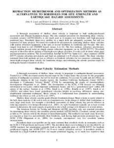
In Table I we compare the present method for the transformation of forces and back-transformation of optimization step during a geometry optimization cycle to the regular technique for a few medium to large molecules, ranging in size from 56 atoms to 642 atoms. Because of the different formalism, the regular method scales as a function of the number of internal coordinates while the new, fast transformation scales as a function of the number of Cartesian coordinates. This is a very significant advantage when the internal coordinate system is highly redundant and allows the effective use of even a full set of distances as coordinates. The plot of the square root of average CPU time spent for the transformations during the optimizations versus the number of atoms ~shown in Fig. 1! confirms that the present method scales as O(N 2atoms). The test molecules have been selected to represent a range of systems, with different structural properties. ~a! Buckminsterfullerene, C60 , has a network of fused five and six membered rings; even an optimization in Cartesian coordinate system should behave satisfactorily for this fairly rigid system. Consequently, only a few optimization cycles are needed from a moderately unsymmetrical geometry ~distorted by a random displacement from the optimized geometry resulting in an root-mean-square ~rms! error of 0.1 Å!. ~b! Taxol is a sizable organic molecule, with a number of fused rings and several rotatible bonds. The present algorithm is more than 200 times faster than the regular transformation, when averaged over the 54 optimization steps. ~c! Ala5 , Ala10 , and Ala20 have been chosen to explore the behavior of the present methodology with increasing size, while keeping the structural properties similar. The peptides form a-helices stabilized by hydrogen bonds and benefit from the use of redundant internal coordinates to describe the potential energy surface. The ratio of the CPU usage using the regular method versus the present algorithm increases essentially linearly with the size of the molecules, not only for the average CPU time per cycle but also for the first optimization cycle. ~d! RNA segments surrounded by water

J. Chem. Phys., Vol. 109, No. 17, 1 November 1998

O. Farkas and H. B. Schlegel

7103

TABLE I. Comparison of the CPU time used for the force and coordinate transformations in each geometry optimization cycle using the regular method and the presented O(N 2 ) technique.a CPU time usage in seconds during geometry optimization

Molecule C60 Taxol For-Ala5-NH2 For-Ala10-NH2 For-Ala20-NH2 RNA1waters Crambinc

No. of No. of atoms coordinates 60 113 56 106 206 368 642

630 668 280 546 1068 1918 2673

Current study

Level of theory

Machine type

Regular

First cycle

Averageb

AM1 AM1 AM1 AM1 AM1 MNDO UFF-MMd

IBM RS6k/560 IBM RS6k/560 IBM RS6k/560 IBM RS6k/560 IBM RS6k/560 IBM RS6k/560 Cray J90

169.81 200.47 8.04 99.51 890.32 5373.43 4672.44

1.59 7.38 1.16 6.53 45.60 331.83 460.40

0.40 ~10! 0.91 ~54! 0.21 ~29! 0.80 ~77! 2.37 ~184! 6.64 ~359! 8.65 ~323!

a

The CPU usage is listed separately for the regular method that uses a generalized inverse, for the O(N 2 ) method for the first optimization cycle and averaged over the number of optimization cycles needed for convergence. All calculations have been carried out using GANSSIAN 98 Rev. A.1 ~Ref. 12!. b Number of optimization steps are in parentheses. c Optimization started from the geometry published in Ref. 13. d Reference 11.

molecules ~8 bases in 4 segments, 4 sodium ions and 34 water molecules! is a problematic test case regardless of the choice of the coordinate system. The optimization had to be restarted a few times to rebuild the coordinate system, because of the reorientation of the water molecules and changes in the network of hydrogen bonds. The data in Table I have been extracted from the last restart which converges to the final optimized structure. The internal coordinate system can be built automatically during the geometry optimization, but this feature has not been used in the current study for the purpose of easier comparison. ~e! Because of the availability of high resolution x-ray structures, the small protein crambin has been used frequently as a test for macromolecular geometry optimizations with molecular mechanics force fields. With recent improvements in the ab initio quantum chemical methods, molecules of this size can be studied and optimized at ab initio Hartree–Fock13 or density functional theory ~DFT! level of theory. Our algorithm is more than 500 times faster for crambin. Even molecules as large as plasminogen

and HIV protease can now be optimized in the framework of redundant internal coordinates.14

V. SUMMARY

This paper outlines an efficient, O(N 2 ) method for performing the coordinate transformations during quantum chemical geometry optimizations. The improvements in speed cause no loss of accuracy and are suitable for any complete, redundant, or nonredundant internal coordinate system. The present method involves three major changes to the regular algorithm: ~1! use of an updated inverse to solve the systems of linear equations, ~2! avoidance of the redundancy problem by transforming the equations into a nonredundant space, and ~3! Gram–Schmidt orthogonalization of the subspace of constrained internal coordinates to remove the overlap with the variable subspace. Further acceleration can be expected for larger molecules by using sparse matrix and limited memory update storage techniques. The use of a conjugate gradient or DIIS15 based optimizer in the algorithm may also speed up the convergence. The algorithm has been implemented as a part of the default optimization method for large molecules into the latest release of the 12 GAUSSIAN series of programs. An O(N 2 ) method for solving of the rational function optimization7 ~RFO! step in geometry optimization will be discussed in a subsequent paper.16 Another potential application of the present coordinate transformation method is in NMR structure determination. This approach is an alternative to the distance geometry methods17 for generating geometries that satisfy distance and other internal coordinate constraints obtained from NMR data.

ACKNOWLEDGMENTS FIG. 1. The square root of the average CPU time spent for the transformation of forces and coordinates in each optimization cycle vs the number of atoms.

This work has been supported by Gaussian, Inc., the Hungarian Research Foundation ~OTKA F-017178!, and the

7104

J. Chem. Phys., Vol. 109, No. 17, 1 November 1998

National Science Foundation ~NSF Grant No. CHE ¨ .F. thanks the Hungarian Fellowship Board for 9400678!. O an Eo¨tvo¨s Fellowship. 1

H. B. Schlegel, in Modern Electronic Structure Theory, edited by D. R. Yarkony ~World Scientific, Singapore, 1995!, pp. 459–500; in Encyclopedia of Computational Chemistry ~Wiley, New York, 1998!. 2 ~a! P. Pulay, G. Fogarasi, F. Pang, and J. E. Boggs, J. Am. Chem. Soc. 101, 2550 ~1979!; ~b! G. Fogarasi, X. Zhou, P. W. Taylor, and P. Pulay, ibid. 114, 8191 ~1992!; ~c! P. Pulay and G. Fogarasi, J. Chem. Phys. 96, 2856 ~1992!; ~d! C. Peng, P. Y. Ayala, H. B. Schlegel, and M. J. Frisch, J. Comput. Chem. 17, 49 ~1996!. 3 L. Greengard and V. Rokhlin, J. Comput. Phys. 73, 325 ~1987!; L. Greengard, The Rapid Evaluation of Potential Fields in Particle Systems ~MIT Press, Cambridge, MA, 1988!; Science 265, 909 ~1994!; C. A. White and M. Head-Gordon, J. Chem. Phys. 101, 6593 ~1994!; J. C. Burant, M. C. Strain, G. E. Scuseria, and M. J. Frisch, Chem. Phys. Lett. 248, 43 ~1996!; M. C. Strain, G. E. Scuseria, and M. J. Frisch, Science 271, 51 ~1996!. 4 J. M. Millam and G. E. Scuseria, J. Chem. Phys. 106, 5569 ~1997!; A. D. Daniels, J. M. Millam, and G. E. Scuseria, ibid. 107, 425 ~1997!. 5 U. Singh and P. A. Kollman, J. Comput. Chem. 7, 718 ~1986!; F. Maseras and K. Morokuma, ibid. 16, 1170 ~1995!; T. Matsubara, S. Sieber, and K. Morokuma, Int. J. Quantum Chem. 60, 1101 ~1996!; M. Svensson, S. Humbel, R. D. J. Froese, T. Matsubara, S. Sieber, and K. Morokuma, J. Phys. Chem. 100, 19357 ~1996!; S. Dapprich, I. Komaromi, K. S. Byun, K. Morokuma, and M. J. Frisch, Theor. Chem. Acc. ~in press!. 6 E. B. Wilson, J. C. Decius, and P. C. Cross, Molecular Vibrations ~McGraw-Hill, New York, 1955!. 7 A. Banerjee, N. Adams, J. Simons, and R. Shepard, J. Phys. Chem. 89, 52 ~1985!.

O. Farkas and H. B. Schlegel 8

W. H. Press, S. A. Teukolsky, W. T. Vetterling, and B. P. Flannery Numerical Recipies in FORTRAN, 2nd ed. ~Cambridge University Press, New York, 1992!. 9 B. Murtagh and R. W. H. Sargent, Comput. J. ~UK! 13, 185 ~1972!; J. E. Dennis and R. B. Schnabel, Numerical Methods for Unconstrained Optimization and Non-Linear Equations ~Prentice Hall, New Jersey, 1983!. 10 C. G. Broyden, J. Inst. Math. Appl. 6, 76 ~1970!; R. Fletcher, Comput. J. ~UK! 13, 317 ~1970!; D. Goldfarb, Math. Comput. 24, 23 ~1970!; D. F. Shanno, ibid. , 647 ~1970!. 11 A. K. Rappe´, C. J. Casewit, K. S. Colwell, W. A. Goddard III, and W. M. Skiff, J. Am. Chem. Soc. 114, 10024 ~1992!. 12 GAUSSIAN 98 ~Revision A.1!, M. J. Frisch, G. W. Trucks, H. B. Schlegel, G. E. Scuseria, M. A. Robb, J. R. Cheeseman, V. G. Zakrzewski, J. A. Montgomery, R. E. Stratmann, J. C. Burant, S. Dapprich, J. M. Millam, A. D. ¨ . Farkas, J. Tomasi, V. Barone, M. Daniels, K. N. Kudin, M. C. Strain, O Cossi, R. Cammi, B. Mennucci, C. Pomelli, G. A. Petersson, P. Y. Ayala, A. D. Rabuck, K. Raghavachari, Q. Cui, K. Morokuma, J. B. Foresman, J. Cioslowski, J. V. Ortiz, V. Barone, B. B. Stefanov, G. Liu, A. Liashenko, P. Piskorz, W. Chen, M. W. Wong, J. L. Andres, E. S. Replogle, R. Gomperts, R. L. Martin, D. J. Fox, T. Keith, M. A. Al-Laham, A. Nanayakkara, C. Y. Peng, M. Challacombe, P. M. W. Gill, B. Johnson, and J. Pople, Gaussian, Inc., Pittsburgh PA, 1998. 13 C. van Alsenoy, C.-H. Yu, A. Peeters, J. M. L. Martin, and L. Scha¨fer, J. Phys. Chem. 102, 2246 ~1998!. 14 G. Scuseria, unpublished data; M. J. Frisch, unpublished data. 15 P. Pulay, Chem. Phys. Lett. 73, 393 ~1980!; P. Pulay, J. Comput. Chem. 3, 556 ~1982!. 16 ¨ O. Farkas and H. B. Schlegel ~to be published!. 17 G. M. Crippen and T. F. Havel, Distance Geometry and Molecular Conformation ~Research Studies Press, UK, 1988!.