3511 The Journal of Experimental Biology 214, 3511-3517 © 2011. Published by The Company of Biologists Ltd doi:10.1242/jeb.057422
METHODS & TECHNIQUES Combining forces and kinematics for calculating consistent centre of mass trajectories Horst-Moritz Maus*, André Seyfarth and Sten Grimmer Lauflabor Locomotion Laboratory, Friedrich-Schiller Universität Jena, Dornburgerstr. 23, D-07743 Jena, Germany *Author for correspondence (
[email protected])
Accepted 19 July 2011
SUMMARY The motion of centre of mass (CoM) is a fundamental object of investigation in biomechanical analysis. In principle, the CoM motion can either be calculated from force data (dynamic method) or motion capture data (kinematic method). In both approaches, the accuracy of the calculated trajectories depends on the quality of the original signals. Interestingly, the inaccuracies in each method are related to different parts of the Fourier spectrum. Here, we present a new approach to compute CoM motion based on the reliable frequency range of force and kinematic measurements. As a result we obtain physically consistent CoM and force signals, i.e. the second derivative of the CoM trajectory equals the force. The algorithm is verified on simulation data and applied to selected experimental data. We show that the new algorithm can eliminate typical inaccuracies inherent in kinematic and force signals. Also, we discuss the biological and technical origins of these findings. Key words: biomechanics, locomotion, gait analysis, CoM, Fourier.
INTRODUCTION
For biomechanical studies on animal and human locomotion as well as for clinical gait assessment, a precise estimation of the body centre of mass (CoM) trajectory is crucial. In general, the CoM motion is calculated either from kinematic data (kinematic method), often by incorporating an anthropometric model, or by double integration of the acceleration obtained from ground reaction forces (GRF; dynamic method). The kinematic methods can be subdivided into pure marker methods and segmental analysis methods. Pure marker methods use a single marker (Saini et al., 1998; Thirunarayan et al., 1996) or a minimalistic marker set (Forsell and Halvorsen, 2009; Halvorsen et al., 2009) to estimate the CoM coordinates. However, some uncertainty arises in these minimalistic estimates because limb motion is not accounted for (Whittle, 1997). The segmental analysis methods rely on full-body marker sets, e.g. Helen–Hayes (cf. Castagno et al., 1995; Kadaba et al., 1990; Sutherland, 2002), and calculates the CoM trajectory by assuming the masses and CoM locations of each segment (Eames et al., 1999). For humans, segmental data are usually obtained from anthropometric literature (Dempster, 1955) or individually determined from a reference measurement (Forsell and Halvorsen, 2009). However, for animals biometric data are much less available. The accuracy of the segmental analyses relies on the correct marker placement and the correct estimation of segment properties (cf. Shan and Bohn, 2003). In addition, potential errors arise from unrecorded dynamics of segment masses, i.e. wobbling masses (Gruber et al., 1998; Günther et al., 2003; Schmitt and Günther, 2010) and motion of the viscera (Minetti and Belli, 1994). In the dynamic method these problems do not occur. According to Newton’s second law, the CoM motion is fully determined by the body’s mass, external forces, the initial velocity and the initial position. Therefore, the accuracy of the dynamic method is limited
by the precision of the measured forces and the precision of the integration constants (Cavagna, 1975). Although the initial position can be estimated quite well, the determination of the initial velocity is a common problem in practice. Gutierrez-Farewik et al. (Gutierrez-Farewik et al., 2006) and Günther and Blickhan (Günther and Blickhan, 2002) showed that the calculated trajectory strongly depends on the body’s mass measurement and the estimated initial velocity. It is possible to optimize the guess for the initial velocity with the path matching method, i.e. the CoM initial conditions are estimated from a reference marker (Daley et al., 2006; McGowan et al., 2005). Yet, as this maker-based criterion itself is only a guess, the optimisation is prone to error. In addition, because of systematic errors in the force signals (Mack, 2007), high-pass filters have to be applied to the force signals for long-term integration of acceleration. Another method to correct the integration constants on a per-stride basis has been proposed by Saibene and Minetti (Saibene and Minetti, 2003). Here, the mean velocity of each stride is replaced by a kinematic estimate, thus attenuating the long-term drift. However, it remains unclear to what extend typical systematic errors in both kinematic and dynamic measurements bias the results. The sources of errors in kinematic and dynamic methods are of a different kind. Although the dynamic method has drawbacks on long-term scales, the kinematic methods do not fully capture some effects on short time scales, e.g. wobbling masses. Thus, typical inherent errors of both methods can be regarded as opposed, resulting in systematic mismatches of kinematic and dynamic CoM estimates (Gard et al., 2004). Gard et al. (Gard et al., 2004) further proposed that a combination of kinematic and dynamic methods could potentially lead to more accurate results. Here, we present a simple yet powerful approach to calculate CoM trajectories from measured kinematic and dynamic data. It is based on the combination of the low-frequency content of kinematic
THE JOURNAL OF EXPERIMENTAL BIOLOGY
3512 H.-M. Maus, A. Seyfarth and S. Grimmer Input
Algorithm
d Kinematic CoM dt estimate
Measured GRF
dt
Kinematic velocity estimate Dynamic velocity estimate
Kinematic velocity spectrum
FFT
dt Weighting function
Dynamic velocity spectrum
FFT
Consistent output
Combined FFT–1 Combined velocity velocity spectrum
Combined CoM position
d dt Combined GRF
Fig.1. Summary of the proposed algorithm. The velocity of the centre of mass (CoM) is computed from a combination of force and kinematic data. The corresponding trajectory and ground reaction force (GRF) are obtained by integration and derivation, respectively. An implementation in MATLAB code can be downloaded from http://www.lauflabor.de in the publications section. FFT, fast Fourier transform.
data and the high-frequency content of GRF to calculate a more accurate CoM velocity. From this velocity, the CoM trajectory and a corrected GRF are calculated by integration and derivation, respectively. Figuratively speaking, this method combines the strengths of both approaches by taking the coarse motion from the kinematic data and adding the fine structure from the GRF. The proposed method is tested on simulation data and subsequently applied to real measurements. The resulting CoM trajectory and GRF are physically consistent and closely resemble the original measurements. MATERIALS AND METHODS
Here, we present the new CoM algorithm and the simulation model used for verification. Further, we describe real measurements to which the algorithm is applied.
•
• •
dependent on the experiment and the equipment. Here, we used a sigmoid function that is close to 0 for low frequencies and close to 1 for high frequencies (Fig.2). Because the Fourier spectrum is symmetric, this function must also be symmetric. For the appropriate selection of the threshold separating high and low frequencies, see Selection of the weighting function and Fig.3. We used the weighting factor w to create a combined spectrum vc(f)w(f)vd(f)+[1–w(f)]vk(f), which is a weighted sum of the low frequencies of the kinematic estimate and the high frequencies of the dynamic estimate. We computed the combined velocity vc as the inverse Fourier transformation of the combined spectrum vc. We computed the combined CoM position and GRF from the combined velocity by integrating or differentiating, respectively. Selection of the weighting function
The CoM algorithm
Weighting function, w
The main idea of the algorithm is to compute the CoM velocity based on kinematic and dynamic velocity estimates, taking only the frequencies of each estimate into account that we consider to be reliable. From this combined velocity, the GRF and CoM trajectory are calculated. The algorithm is summarized in Fig.1. The individual steps are as follows and hold for each coordinate separately: • We computed two estimates of the CoM velocity, a kinematic estimate vk, by differentiating the kinematic CoM estimate, and a dynamic estimate vd, by integrating the GRF (taking gravity and body mass into account). Here, it is important that the mean force is accurate. For a subject standing at the beginning and the end of a trial, we set the mean force to exactly zero, because here the mean GRF exactly compensates gravity. • We computed the Fourier transform vk and vd of the kinematic and dynamic velocity estimates, respectively. • We selected a weighting factor w between 0 and 1 as a function of the frequency, i.e. w(f) expressing the confidence in each method with respect to the frequency. The choice of w can be
Some parts of the segment dynamics, primarily the composition of soft and rigid body structures, are not well recorded in the kinematics. As this segment-internal motion, i.e. motion of the soft tissue with respect to the bone, mainly affects harmonics of the stepping frequency and higher frequencies (Günther et al., 2003), we expect the part of motion concerning frequencies below a certain threshold to be well captured, and that this threshold is not substantially lower than the stepping frequency. In contrast, errors in force measurement usually are of a type that mainly affects low frequencies, e.g. drift and slowly varying offset (Mack, 2007; Nigg and Herzog, 1999). This is why integration of acceleration obtained from measured GRF without filtering gives reasonable results only if trials are short, i.e. if very low frequencies are not present. However, we have no reason to assume systematic errors in the force measurement at high frequencies. An exception may be the eigenfrequency of the measurement system. In our system, the eigenfrequency is 120Hz, which corresponds roughly to the 40th harmonic of the stepping frequency and thus is far out of the region of interest (Racic et al., 2010). Fig.2. The selected weighting function expresses the relative reliability of the signals expressed in the frequency domain. We chose a sum of two sigmoid functions, w1/{1+exp[–(f–f0)s]} + 1/(1+exp{–[(fs–f0)–f]s}), w(0)0, with fs and f0 denoting the sampling frequency and threshold frequency, respectively. The steepness of the slope was s10Hz–1.
1
Threshold frequency 1.5 Hz
0.5
0 0
1
2
3
4 996 Frequency (Hz)
997
998
999
1000
THE JOURNAL OF EXPERIMENTAL BIOLOGY
Consistent CoM and force calculation 4.0 log10 ⱍvelocity spectrumⱍ
3.5
Normalized sum-of-squares
3.0 2.5
Errors in force dominate
Errors in kinematics dominate
2.0 Optimal threshold
1.5 1.0 0.5 0 0
1
2
3
4
5
Frequency (Hz)
These arguments lead us to use a weighting function that takes low frequencies from the kinematics and higher frequencies from the dynamics. As we expect that the wobbling masses move approximately with the frequency of the driving force (i.e. the stepping frequency) and their harmonics, we assume that a threshold frequency slightly below the dominant frequency of the motion would be optimal. The validity of this argument is strongly supported by our simulation results, as shown in Fig.3. Verification using simulated data
In order to verify the accuracy of the CoM estimate, we used a simulation model of a bipedal walker to create an artificial dataset with precisely known dynamics. Subsequently, we added virtual measurement errors that resemble errors we expect from realworld measurements, including errors concerning the wobbling masses.
3513
Fig.3. To assess the accuracy of the CoM estimation, the residual sum of squares with respect to the real CoM motion of the model was calculated as a function of the threshold frequency (black diamonds). The values were normalized to the apparent plateau after the dominant motion (2.5Hz). Additionally, the amplitude of the velocity spectrum is shown (solid grey line). The optimal threshold frequency is slightly below the dominant frequency of the motion. Therefore, a reasonable threshold frequency should be selected below this dominant frequency. In this case, appropriate threshold frequencies approximately range from 1.0 to 1.6Hz. If the threshold is below or above this range, errors in the measured force or measured kinematics become dominant and decrease the estimation quality.
respectively; A is amplitude (5N); i and ⬘i are gaussian random numbers with zero mean and unit variance; Fi⬘ is the scaled GRF; and Fi0 is the real GRF in units of body weight. The index i denotes the particular sampling frame. Then, the virtually measured force is FimFi⬘+Ri1+Ri2. The dynamic estimate of the CoM was computed by a double integration of the acceleration obtained from GRF, thereby applying a 0.35Hz high-pass filter for the force and obtained velocity. The cut-off at 0.35Hz was chosen because in this model it resulted in the most accurate CoM reconstruction. Lower cut-offs led to increased long-term oscillation whereas higher cut-offs led to an underestimation of the oscillation amplitude. For the CoM estimation using the proposed algorithm, the threshold frequency was set to 1.5Hz, which is below the dominant frequency of the motion at 1.64Hz. Analysis of experimental data
Model description
We used the model of a human walker (mass80kg) from Geyer and Herr (Geyer and Herr, 2010), which is able to predict typical human-like GRF, CoM motion and even muscle activation patterns. We modified this model by setting S of each segment’s mass to a wobbling mass, which is connected to the segment by a springdamper element [roughly according to Minetti and Belli (Minetti and Belli, 1994)]. The spring and damping constants are chosen such that the eigenfrequency is ~10Hz for the limbs and ~3Hz for the head–arms–trunk segment, with a decay time of 0.4s. Our modified model walked in an aperiodic manner with a dominant motion frequency of 1.64Hz. Data were sampled every 1ms simulation time. Virtual measurement errors and CoM estimation
The kinematic CoM estimate of the model was computed using standard segmental analysis (Winter, 2009), including only measurements of the position of the rigid segments, and neglecting wobbling masses. Additionally, white noise with a r.m.s. of 0.5mm was added. The force data were modified by: (1) adding a non-stationary noise signal with amplitude of 5N; (2) adding white noise with a r.m.s. of 5N; and (3) applying a small nonlinear scaling. In detail, these corruptions were calculated to: (1) Ri1Asin(⌺1i0.01i), (2) Ri2A⬘i and (3) Fi⬘0.98(Fi0)1.02, where Ri1 and Ri2 are random non-stationary and stationary noise,
In order to demonstrate the new method, we calculated the CoM trajectories of human running and walking and compared these with kinematic and dynamic CoM estimates. We further calculated the ‘kinematic GRF’ as second derivative of the kinematic CoM estimate to compare kinematic GRF, measured GRF and calculated GRF. Measurement setup and protocol
All measurements were conducted on an instrumented custom-built treadmill (ADAL, HEF Medical Development, AndrezieuxBoutheon, France). We further used a marker-based kinematic system (Qualisys, Gothenburg, Sweden) to capture the subject’s motion. Force data were sampled at 1000Hz; kinematics were sampled at 240Hz. The subject walked at 1.8ms–1 and ran at 2.7ms–1 on the treadmill. Each trial started and ended with 5s of quiet standing. The total trial duration was 50 and 55s, respectively. Data pre-processing
A linear drift in the total vertical and total horizontal force was removed from the raw data. Kinematic data were linearly interpolated from 240 to 1000Hz to match the treadmill sampling frequency. We do not expect relevant numerical errors from the interpolation because we used only kinematic frequencies up to ~1.5Hz, which are well over-sampled and thus hardly affected by this interpolation.
THE JOURNAL OF EXPERIMENTAL BIOLOGY
3514 H.-M. Maus, A. Seyfarth and S. Grimmer
A
B Kinematic method Dynamic method Combined Real
–0.01 –0.02 –0.03 –0.04
1.09 Vertical position (m)
Summed abs. error (a.u.)
Vertical displacement (m)
0
0
20
40 60 Time (% gait cycle)
80
100
0
2
4 6 Time (gait cycle)
8
10
C
1.07
1.05 29
30
31 32 Horizontal position (m)
33
34
Fig.4. Comparisons of the real model CoM and the different calculation methods. (A)Simulation results for the real, measured and reconstructed time courses of the vertical CoM over one gait cycle. For better comparison, only the displacement relative to the initial (apex) position is shown. (B)The accumulated absolute errors over 10 strides. The error in the kinematic estimate accumulates regularly, whereas the error in the dynamic method accumulates unregularly (see e.g. t~3.5 gait cycles). This behaviour is due to the different nature of the errors. (C)Sagittal plane movement of the CoM. The kinematic estimate has a systematic incorrect shape, but it keeps track of the motion well. The opposite is true for the dynamic estimate. The combined estimate performs best as it keeps track of the motion and also shows good match of the shape.
CoM estimation: kinematic, dynamic and new method
The kinematic CoM estimate was obtained using a standard segmental analysis (Winter, 2009). Corresponding GRFs were calculated by computing the second derivative of the CoM estimate after applying a second-order Butterworth filter with a cut-off frequency of 15Hz. The dynamic CoM estimate was obtained by twice integrating the GRF. To avoid spurious drifts in the resulting trajectory, components below 0.35Hz were removed before integration by applying a first-order Butterworth filter to GRFs and computed velocity. Finally, we applied the proposed algorithm to calculate the combined CoM and GRF. We used the measured GRF and the kinematic CoM estimate as inputs for the algorithm. The threshold frequency was set to 1.5Hz. RESULTS AND DISCUSSION
The analysis of the simulated model shows that the proposed method reconstructs the CoM motion with greater accuracy than the pure kinematic or dynamic methods (Fig.4). For better visual comparison, only the displacement relative to the first apex position is shown in Fig.4A. Also, we applied the new method to the forward motion. The results show a proper tracking of the motion (Fig.4C). The differences of the kinematic estimate are apparent in every step, whereas, because of the tracking problem, the dynamic method accumulates the error in the long term (Fig.4B). These slow drifts are not present in the combined estimate. The results of applying the algorithm to walking and running data are shown in Fig.5. Here, we focused on the vertical CoM
component, but the method is applicable to any CoM component. The calculated data resemble both the kinematic CoM estimate and the measured GRF. Because of this and its inherent physical consistency (i.e. the combined GRF equals the second derivative of the combined CoM minus gravity), this method provides a suitable enhancement to common kinematic CoM estimations. These consistent data can then be used for further analysis, e.g. of external work and external power, with greater confidence. Our results show systematic deviations of the GRF obtained directly from kinematics compared with the measured GRF. This comprises mainly an underestimation of the GRF after lift-off in running, which is accompanied by an overestimation of the GRF during stance (Fig.5). Similar results were shown by Racic et al. (Racic et al., 2010). As negative vertical GRF cannot occur in typical running and hopping experiments, this indicates a systematic shortcoming of kinematic GRF estimates, which also extends to the corresponding CoM estimate according to Newton’s second law. The combined CoM/GRF estimates do not show this systematic deviation but closely resemble the measured forces. In the Appendix, we show that this property also holds for very simple kinematic CoM estimations, such as a single marker, both in human walking and dog trotting. Thus, accurate CoM trajectories can be obtained without knowing segment properties using this algorithm. Further, this also allows highly reduced experimental effort for some gait analyses. The proposed method also accounts for wobbling masses (Gruber et al., 1998; Günther et al., 2003; Schmitt and Günther, 2010) because their motion is included in the GRF. Wobbling masses are not necessarily captured by the kinematic
THE JOURNAL OF EXPERIMENTAL BIOLOGY
Consistent CoM and force calculation Walking 1.8 m s–1
Vertical displacement (m)
0.02
3515
Running 2.7 m s–1
0 –0.02 –0.04 –0.06
Kinematic method Dynamic method Combined
–0.08
Force (BW)
2.5 2.0 1.5 1.0 0.5 0 0
20
40
60
80
100 0 20 Time (% gait cycle)
40
60
80
100
Fig.5. Results of applying the new algorithm (grey solid line) to human walking and running in comparison to the classic approaches. Shown are the vertical CoM motion and the derived GRF for one gait cycle. In general, the kinematic estimate shows slightly larger oscillation than the dynamic and combined estimates of the CoM trajectory. This is also reflected in differences in the corresponding GRF, indicating that this systematic deviation is a shortcoming of the kinematic estimate. The difference between the dynamic and the combined estimate, i.e. smaller oscillation amplitude in the dynamic estimate, is in agreement with the simulation results.
measurement. This can lead to differences especially when the wobbling mass motion is substantial or out of phase with respect to the skeletal motion (Minetti and Belli, 1994). Conversely, it appears plausible that this soft tissue motion could be estimated by calculating the difference of the calculated CoM and the kinematic CoM estimate. Thus, this method could also provide a basis for analyzing soft tissue motion. A standard method in engineering to combine both kinematic and dynamic input to obtain a more reliable CoM estimate is the Kalman filter (Kalman, 1960). Roughly speaking, the main idea is to propagate the trajectory based on a system model using the GRF as input [so-called estimate xi–f(xi–1+, GRF)], and updating this estimate with each measurement yi of the CoM trajectory,
Kinematic method
Vertical CoM position (m)
1.00
Standing
xi+x–+K(yi–xi–). The relative weight K of the update is based on the relative confidence in the estimate and the measurement. Under certain restrictions of the measurement errors, the Kalman filter or its modifications give an optimal estimation. However, this does not apply here as both the kinematic and GRF measurement errors have a systematic structure that renders them very different from these restrictions. In order to use Kalman filtering here, a model of the measurement errors would have to be included. In contrast, the proposed method offers a convenient and intuitive way, namely the selection of a threshold frequency, to account for the typical structure in the measurement errors. Physical consistency in long trials can also be obtained by the dynamic method, when low frequencies are discarded. When low
Dynamic method
Walking
Combined
Running
Walking
Standing
0.98 0.96 0.94 0.92 0.90 2
4
6
8
10
12
14 38 Time (s)
40
42
44
46
48
THE JOURNAL OF EXPERIMENTAL BIOLOGY
Fig.6. Results of different CoM methods for a 55s trial with standing, walking and running. Comparing the dynamic estimate of the CoM trajectory with kinematic and combined CoM trajectories during the running trial shows the drawback of discarding the low-frequency parts (here