USING MAPINFO VERTICAL MAPPER INTERPOLATION TECHNIQUES FOR.
ESTONIAN OIL SHALE RESERVE CALCULATIONS. INGO VALGMA, Dr. Eng.
USING MAPINFO VERTICAL MAPPER INTERPOLATION TECHNIQUES FOR ESTONIAN OIL SHALE RESERVE CALCULATIONS INGO VALGMA, Dr. Eng. Mining Department of Tallinn Technical University, Kopli 82, Tallinn, 10412, Estonia, http://www.ttu.ee/maeinst/ Phone: +372 620 38 50, Fax: + 372 620 36 96, E-mail:
[email protected] Summary A digital map of Estonian oil shale mining was created for joining data of technological, environmental, and social limitations in the deposit with area of 2900 km2. For evaluating potential resource of oil shale its amount, tonnage and energy were calculated. Then the quantity of economical oil shale for power plants and shale oil resource were calculated. Seam thickness was interpolated from analyzed and calculated data points of the oil shale seam and a model was created for visual control. Calculating and interpolating energy rating per square metre is necessary for energy resource evaluation. Energy rating is the most important factor for determining oil shale reserve in the case of using it for electricity generation. In the case of oil production, figures of oil yield and resource in oil shale are the most important figures for determining the value of the deposit. Basing on the models, oil resource has been calculated. Choosing between various interpolations showed that Inverse Distance Weighting gives the most reliable figures for oil shale tonnage with available data. Natural Neighbor Regions and Kriging are the more suitable methods when using detailed data.
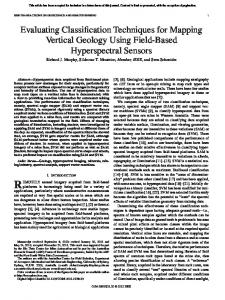
Introduction Oil shale bed in Estonia is deposited in the depth of 0…100 m with the thickness of 1.4…3.2 m in the area of 2884 km2 (Figure 1). The mineable seam consists of seven kukersite layers and four to six limestone interlayers. The layers are named A…F1. The energy rating of the bed is 15…45 GJ/m2. Kunda outc0ro
Gulf of Finland
p
Kohtla-Järve Rakvere
Sillamäe
Jõhvi
Kiviõli
Narva-Jõesuu Narva
Russia
Estonia
Mined out area
Tapa
Exploration fields Lääne-Viru county 4
Ida Viru county
0
25
50
Lake Peipus
Järva county
kilometres
Jõgeva county
Figure 1 Baltic oil shale area
M
t
Oil shale mining in Estonia province started in 1916, it was extracted in surface mines using the opencast method. Underground mining started in 1922. Room-and-pillar mining, which is the only underground oil shale mining method today, started in 1960. During the years 1971…2001 longwall mining with shearers was used in some of the mines. In total ten oil shale surface mines and 13 underground mines have been in operation. Probability of opening new operations is high in the case if oil shale processing or cement productions are becoming more active.
The criteria of the oil shale reserve The criteria of the oil shale reserve are energy rating, calorific value of the layers, thickness and depth of the seam, location, available mining technology, world price of competitive fuel and its transporting cost, oil shale mining and transporting cost. In addition, nature protection areas are limiting factors for mining. The economic criterion for determining Estonia’s kukersite∗ oil shale reserve for electricity generation is the energy rating of the seam in GJ/m2. It is calculated as the sum of the products of thickness, calorific values and densities of all oil shale layers A-F1 and limestone interlayers. A reserve is mineable when energy rating of the block is at least 35 GJ/m2 and subeconomic if energy rating is 25…35 GJ/m2. According to the Balance of Estonian Natural Resources, as an example the oil shale reserve was 5 billion tonnes in the year 2000. Economic reserve was 1.5 billion t and subeconomic 3.5 billion t (Table 1). These figures apply to oil shale usage for electricity generation in power plants and are calculated only by oil shale layers, which is fiction because in most cases total bed is used for combustion. In the case of wide-scale using of oil shale for cement or oil production, the criteria must be changed. Table 1 Oil shale reserve Reserve Economic Proved Probable Subeconomic In nature protection areas In pillars subeconomic Total
Tonnage, bill t 1.5 1.2 0.3 3.5 1.3 0.2 2.0 5
Energy rating, GJ/m2 >35
25...35
>25
Percentage 30 24 6 70 26 4 40 100
Modeling In total 375 data points have been used for modeling (Figure 2). Every data point represents data of one reserve block with 5 to 15 drill holes and has been taken as an average for an area about seven km2.
∗
In addition to kukersite oil shale in Estonia, there are occurrences of another kind of oil shale – dictyonema argillite, mined and used in Sillamäe for extracting uranium in 1948…1953.
Konnu1 Konnu3
Haljala1+5 Haljala4 1 4 8 12 17 22 27 33 106
126
3 6 10 14 19 24 29 35 40 45 51 57 63 71 79 88 97 107
127
7 11 15 20 25 30 36 41 46 52 58 64 72 80 89 98 108
128
147
166
184
16 21 26 31 37 42 47 53 59 65 73 81 90 99 109
129
148
167
185
2 5 9 13 18 23 28 34 39
50 56
156 M3
32 38 43 48 54 60 66 74 82 91 100
120
140
159
177
192
44 49 55 62 67 75 83 92 101
121
141
160
178
193 KC
61 68 76 84 93 102
122
142
161
179
KA1
69 77 85 94 103
123
143
162
180
70 78 86 95 104
124
144
163
181
87 96 105
125
145
164
10x10km
136
155
KB4
KC 182 KC2-2 174
Figure 2 Map of source data from geological investigation. Contours show exploration fields. The northern border of the deposit is an outcrop line
Basing on geological data, several grids of oil shale layers and seam were created - those of the height, thickness, in-place tonnage, energy rating, overburden thickness and stripping coefficient. Oil shale resource For evaluating potential resource of oil shale, its amount, tonnage and energy must be calculated. Then the quantity of economical oil shale for power plants and shale oil resource is calculated. It is necessary to follow the criteria for choosing the most appropriate interpolation method. It is not possible to choose right interpolation method beforehand because of numerous options of methods and criteria. Appropriate methods for every operation will be established during calculations. Seam thickness was interpolated from 375 calculated data points of the oil shale seam and a model was created for visual control. Assuming that Estonian oil shale deposit is a combination of current exploration fields, the polygon shown in Figure 3 marks the deposit border covering 2884 km2. The quantity of the oil shale seam could be calculated by extracting thickness and corresponding areas from the created isopachs using SQL query. Inverse distance weighting, triangulation with smoothing, natural neighbor, rectangular interpolation and Kriging methods could be used for interpolation. Reliable data allow to use Voronoi diagram, triangulation and rectangular interpolation. Unreliable data require Inverse Distance Weighting and Kriging. All criteria are summarized in Table 2. Shaded rows show suitable criteria for calculating oil shale tonnage. Natural neighbor is the most suitable method because the initial data were subjectively interpreted average values of exploration blocks. Inverse Distance Weighting Interpolation can also be used because the errors of the initial data exceed smoothing level of the method. Smoothed isopleths give a more clear overview of the deposit and allow extrapolate the data beyond the data points. Table 2 Criteria for choosing interpolation methods. Marks show suitable methods for specific data. Shaded rows show suitable criteria for calculating oil shale tonnage Method Specific data Inverse Triangular Natural Rectangular Kriging Distance Irregular Neighbour interpolation Weighting Network regions Criterion (IDW) (TIN) (NN) ! ! Height Seam height and thickness ! ! Soil chemistry Calorific value, specific
Reliable data Unreliable data Even spacing
Irregular clustered spacing Regular spacing Linear pattern
Interpolation speed is a factor Interpolation speed is not a factor Minimum and maximum values can overshoot the original data Minimum and maximum values can not overshoot the original data Smoothing Result
gravity Analysed data of geological exploration Non-analysed drill hole data Exploitation and exploration drill hole data, same block Exploitation and exploration drill hole data, separate blocks 4x4 km grid calculated by Kattai Drill holes along the forest trails Drill holes along the roads Whole dataset of drill holes
!
!
!
!
!
!
!
!
!
! ! !
!
!
!
!
!
!
!
! !
Average values of the blocks !
Height, thickness
Mining dynamics, technology, landscape situation
!
Using block averages Tonnage calculation
! 3
!
!
!
! 5
3
!
!
0
3
Calculating and interpolating energy rating per square meter is necessary for energy resource evaluation. The graph based on the model (Figure 3) shows the energy ranges of mined oil shale in the deposit, its quantity already mined out and the available resource. Most of mined out oil shale seam has had energy rating more than 35 GJ/m2 (Figure 4). Energy rating of the seam is used as an essential argument for economical calculations. 25
27
23
47 29 21
33
37
45 45 43 39
43
41 33
41
39
37
35 31 10x10km
27 25
Figure 3 Energy rating of oil shale, GJ/m2. The resource over 35 GJ/m2 is economic reserve. Bold conurs in north show mined out area.
10000
8000
15
Oil shale resource, PJ (10 J)
9000
7000 6000 5000 4000 3000 2000 1000 0
21
23
25
27
29
31
33
35
37
39
41
43
45
47
Mined out PJ
0
0
0
0
37
0
7
382
1465
1219
2790
4570
6451
362
Unmined PJ
570
9923
9340
7939
7150
6628
6844
6886
5704
5097
4047
3630
768
0
Energy rating of oil shale, GJ/m2
Figure 4 Oil shale resource in Estonian deposit on PJ. Most of the mined out seam has contained energy more than 35 GJ/m2
Models enable to present the graphs of energy rating showing its extent and ranges. Energy rating is the most important factor for determining oil shale reserve in the case of using it for electricity generation. In the case of oil production, figures of oil yield and resource in oil shale are the most important figures for determining the value of the deposit. Basing on the models, oil resource has been calculated and is presented in Figure 5. 250
Oil resource, Mt
200
150
100
50
0
0,4
0,45
0,5
0,55
0,6
0,65
0,7
0,75
0,8
0,85 14
Mined out Mt
0
0
1
0
2
24
34
85
151
Unmined Mt
140
247
187
170
173
156
127
94
48 0 Oil yield, t/m2
Figure 5 Shale oil resource, Th t in ranges of oil yield
Choosing between various interpolation methods showed that Inverse Distance Weighting (IDW) gives the most reliable figures for oil shale tonnage with available initial data. Natural Neighbor regions (NN) and Kriging are the more suitable interpolation methods when using more detailed data and blocks. Rectangular Interpolation is unsuitable in the case of irregular
mesh of the initial data. All methods give 2,3m for average oil shale thickness except rect. interpolation that gives 2,1m and 11% deviation. Other methods give deviation from 1 to 3 %, which are smaller than errors of initial data. Results of the study The main results are data models of the deposit such as isopleths and 3D drawings of mining conditions like seam thickness, seam depth, calorific value of oil shale and oil yield. The main possible calculations basing on oil shale bedding models are choosing optimum mining location, dynamics and statistics of the mining phenomenon, evaluation of oil shale quantity, energy and oil reserve. Inverse Distance Weighting method gives satisfactory data for the deposit overview (Table 3), other suitable methods can be used for modeling with all initial drill hole data in case of resource calculations in specific location. Table 3 Data of Estonian oil shale deposit. Calculated with inverse distance weighting method.
Indicator
Unit
Unmined
%
Mined out
%
Total or average
2
2476 10139
86% 84%
409 1900
14% 16%
2884 12039
2
4,1
98%
4,6
111% 4,2
3
1,8
101% 1,7
96%
1,8
5657 74524
84% 81%
1116 17283
16% 19%
6774 91808
95% 81%
42 311
133% 32 19% 1652
95% 96%
0,76 0,16
133% 0,57 119% 0,14
Area Oil shale tonnage
km Mt
In-place tonnage
t/m
Specific weight
t/m
3
Quantity Energy
Mm PJ
Energy rating Oil resource
GJ/m 30 Mt 1342
Oil yield per m Oil yield
2
2
2
t/m t/t
0,54 0,13
This study is financed by EstSF Grant No. 4870 Oil Shale Resource. References References and additional information on Estonian oil shale can be found on page http://www.ttu.ee/maeinst/mgis 1. 2. 3.
4. 5.
Valgma I. Geographical Information System for Oil Shale Mining - MGIS. Thesis on Mining Engineering. http://www.ttu.ee/maeinst/mgis Tallinn Technical University. 2002 Valgma, I., Map of oil shale mining history in Estonia, Proc. II. 5th Mining History Congress, Greece, Milos Conference Centre- George Eliopoulos, 2001, 198…193 Valgma I. Mapping potential areas of ground subsidence in Estonian underground oil shale mining district. Proceedings of the 2nd International Conference “Environment. Technology. Resources”. Rezekne, Latvia 25-27 June 1999, 227...232 Valgma I. Post-stripping processes and the landscape of mined areas in Estonian oil shale open-casts. Oil Shale, 2000, Vol. 17, No. 2, 201…212 Valgma I. Using MapInfo Professional and Vertical Mapper for mapping Estonian oil shale deposit and analysing technological limit of overburden thickness. Proceedings of International Conference on GIS for Earth Science Applications, Institute for Geology, Geotechnics and Geophysics, Slovenia Ljubljana 17.-21. May 1998, 187…194