advanced image and video interpolation techniques ... - MacSphere

ADVANCED IMAGE AND VIDEO INTERPOLATION TECHNIQUES BASED ON NONLOCAL-MEANS FILTERING


BY ROOZBEH DEHGHANNASIRI, B.Sc.

a thesis submitted to the department of electrical & computer engineering and the school of graduate studies of mcmaster university in partial fulfilment of the requirements for the degree of Master of Applied Science

c Copyright by Roozbeh Dehghannasiri, July 2012

All Rights Reserved

Master of Applied Science (2012)

McMaster University

(Electrical & Computer Engineering)

TITLE:

Hamilton, Ontario, Canada


AUTHOR:

Roozbeh Dehghannasiri B.Sc., (Electrical Engineering) University of Tehran, Tehran, Iran

SUPERVISOR:

Dr. Shahram Shirani

NUMBER OF PAGES:

xvi, 124

ii

To my beloved family

Abstract In this thesis, we study three different image interpolation applications in high definition (HD) video processing: video de-interlacing, frame rate up-conversion, and view interpolation. We propose novel methods for these applications which are based on the concept of Nonlocal-Means (NL-Means). In the first part of this thesis, we introduce a new de-interlacing method which uses NL-Means algorithm. In this method, every interpolated pixel is set to a weighted average of its neighboring pixels in the current, previous, and the next frames. Weights of the pixels used in this filtering are calculated according to the radiometric distance between the surrounding areas of the pixel being interpolated and the neighboring pixels. One of the main challenges of the NL-Means is finding a suitable size for the neighborhoods (similarity window) that we want to find radiometric distance for them. We address this problem by using a steering kernel in our distance function to adapt the effective size of similarity window to the local information of the image. In order to calculate the weights of the filter, we need to have an estimate of the progressive frames. Therefore, we introduce a lowcomputational initial de-interlacing method. This method interpolates the missing pixel along a direction based on two criteria of having minimum variation and being used by the above or below pixels. This method preserves the edge structures and yields superior visual quality compared to the simple edge-based line-averaging and many other simple iv

de-interlacing methods. The second part of this thesis is devoted to the frame rate up-conversion application. Our frame rate up-conversion method is based on two main steps: NL-Means and foreground/background segmentation. In this method, for every pixel being interpolated first we check whether it belongs to the background or foreground. If the pixel belongs to the background and the values of the next and previous frames’ pixels are the same, we simply set the pixel intensity to the intensity of its location in the previous or next frame. If the pixel belongs to the foreground, we use NL-Means based interpolation for it. We adjust the equations of the NL-means for frame rate up-conversion so that we do not need to have the neighborhoods of the intermediate for calculating the weights of the filter. The comparison of our method with other existing methods shows the better performance of our method. In the third part of this thesis, we introduce a novel view interpolation method without using disparity estimation. In this method, we let every pixel in the intermediate view be the output of the NL-means using the pixels in the reference views. The experimental results demonstrate the better quality of our results compared with other algorithms which use disparity estimation.

v

Acknowledgements It is my great pleasure to thank all people who made this achievement possible. First and foremost, I would like to offer my sincerest appreciation to my supervisor, Dr. Shahram Shirani, without whose knowledge, effort, encouragement, and patience, this thesis would not have been completed. I also thank my friends and colleagues for helping me in my study and making my experience in Hamilton unforgettable. Last but not least, my deepest gratitude and love go to my mother, my father, and my brother, Razi, for their devotion and support through all stages of my life. I would like to dedicate this work to them.

vi

Notation and abbreviations γ

Scaling parameter of steering kernel

Fˆ t0

De-interlaced frame at time t0 by the NL-means method

fˆ(·)

Final estimated pixel by the NL-means method

D

Local gradient matrix

Fit

Interlaced frame at time t

Gt

Noisy frame at time t

I

Interlacing matrix

Nm,t

Similarity window around pixel at position m and time t

Pm

Patch extraction matrix around pixel at position m

σ

Elongation parameter of steering kernel

θ

Dominant orientation angle of steering kernel

εi

iid zero-mean noise value

c(·)

Distance function for the calculation of the NL-means weights vii

E(·)

Energy Function for the NL-means algorithm

f (·)

Original Pixel

f ela (·) De-interlaced pixel by the proposed ELA method f la (·) De-interlaced pixel by the line-averaging method g(·)

Noisy pixel

h

Degree of the NL-means filtering

w(·)

Weights of the regression method

z(·)

NL-means normalizing constant

viii

Contents

Abstract

iv

Acknowledgements

vi

1

Introduction

1

1.1

Literature Review . . . . . . . . . . . . . . . . . . . . . . . . . . . . . . .

3

1.2

Thesis Contributions . . . . . . . . . . . . . . . . . . . . . . . . . . . . .

8

1.2.1

Video De-Interlacing . . . . . . . . . . . . . . . . . . . . . . . . .

8

1.2.2

Frame Rate Up-Conversion . . . . . . . . . . . . . . . . . . . . . .

9

1.2.3

View Interpolation . . . . . . . . . . . . . . . . . . . . . . . . . . 10

1.3 2

Organization . . . . . . . . . . . . . . . . . . . . . . . . . . . . . . . . . . 10

Video De-Interlacing Using Nonlocal-Means

11

2.1

Overview . . . . . . . . . . . . . . . . . . . . . . . . . . . . . . . . . . . 12

2.2

Nonlocal-Means Algorithm . . . . . . . . . . . . . . . . . . . . . . . . . . 17

2.3

2.2.1

Basics of the Nonlocal-Means . . . . . . . . . . . . . . . . . . . . 17

2.2.2

Nonlocal-Means for De-Interlacing . . . . . . . . . . . . . . . . . 20

Proposed De-Interlacing Method . . . . . . . . . . . . . . . . . . . . . . . 27 2.3.1

Initial Estimation . . . . . . . . . . . . . . . . . . . . . . . . . . . 27 ix

2.3.2 2.4

2.5 3

Experimental Results . . . . . . . . . . . . . . . . . . . . . . . . . . . . . 37 2.4.1

Objective Evaluation . . . . . . . . . . . . . . . . . . . . . . . . . 39

2.4.2

Subjective Evaluation . . . . . . . . . . . . . . . . . . . . . . . . . 42

2.4.3

Computational Complexity . . . . . . . . . . . . . . . . . . . . . . 52

Conclusion . . . . . . . . . . . . . . . . . . . . . . . . . . . . . . . . . . 53

Frame Rate Up-Conversion Based on Nonlocal-Means

54

3.1

Overview . . . . . . . . . . . . . . . . . . . . . . . . . . . . . . . . . . . 55

3.2

Proposed Frame Rate Up-Conversion Method . . . . . . . . . . . . . . . . 60

3.3

3.4 4

Locally-Adaptive Nonlocal-Means Filtering . . . . . . . . . . . . . 31

3.2.1

Foreground/Background Separation . . . . . . . . . . . . . . . . . 60

3.2.2

Nonlocal-Means Based Frame Interpolation . . . . . . . . . . . . . 64


Objective Evaluation . . . . . . . . . . . . . . . . . . . . . . . . . 70

3.3.2

Subjective Evaluation . . . . . . . . . . . . . . . . . . . . . . . . . 73

3.3.3

Computational Complexity . . . . . . . . . . . . . . . . . . . . . . 78

Conclusion . . . . . . . . . . . . . . . . . . . . . . . . . . . . . . . . . . 80

View Interpolation Without Explicit Disparity Estimation

81

4.1

Overview . . . . . . . . . . . . . . . . . . . . . . . . . . . . . . . . . . . 81

4.2

Proposed View Interpolation Method . . . . . . . . . . . . . . . . . . . . . 86

4.3


4.4

Computational Complexity Analysis . . . . . . . . . . . . . . . . . 104

Conclusion . . . . . . . . . . . . . . . . . . . . . . . . . . . . . . . . . . 107

x

5

Conclusion and Future Works 5.1

108

Future Works . . . . . . . . . . . . . . . . . . . . . . . . . . . . . . . . . 109

xi

List of Figures 2.1

Video frames with different scanning formats. (a) Interlaced frame. (b) Progressive frame.

2.2

De-interlacing.

2.3

Examples of self-similarities in the images. (a) Coastguard. (b) Foreman.

2.4

Patch extraction.

2.5

An example of the search region and similarity window. (a) A search region in the previ-

13

. . . . . . . . . . . . . . . . . . . . . . . . . . . . . . . . . . 14 . . . . . . . . 19

. . . . . . . . . . . . . . . . . . . . . . . . . . . . . . . . . 22

ous, current and the next frames surrounded by the red square. (b) A similarity window surrounded by the red square.

2.6

. . . . . . . . . . . . . . . . . . . . . . . . . . . 26

Eight different directions that we use to find the initial estimate. The red arrows show the five spatial directions and the green arrows show the three temporal directions.

2.7

. . . . . . 28

The flowchart of the modified edge-based line averaging method that we used as our initial de-interlacing. One branch of the flowchart is for the case that the initial minimum variation direction is temporal, and another one is for the case that the initial minimum variation direction is near-horizontal. The final direction is the direction that we finally decide to interpolate the missing pixel along it.

2.8

. . . . . . . . . . . . . . . . . . . . 32

The fundamental image patches and their corresponding kernel matrices. (a) Texture region. (b) 45 Degree. (c) Vertical edge. (d) Smooth region. (e) -45 Degree. (f) Horizontal edge.

2.9

. . . . . . . . . . . . . . . . . . . . . . . . . . . . . . . . . . . . . . 36

The block diagram of the proposed de-interlacing method.

xii

. . . . . . . . . . . . . . . 37

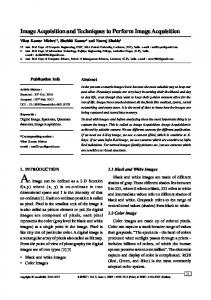
2.10 The results of the proposed de-interlacing method for different video frames. For each pair of the images, the left one is the original image and the right one is the de-interlaced image. (a) and (b) the 131th frame of the Coastguard [PSNR: 36.54 dB]. (c) and (d) the 30th frame of the Stefan [PSNR: 37.72 dB]. (e) and (f) the 150th frame of the Silent [PSNR: 45.18 dB]. (g) and (h) the 142th frame of the Mother [PSNR: 48.42 dB]. (i) and (j) the 60th frame of the Mobile [PSNR: 30.85 dB]. (k) and (l) the 30th frame of the Foreman [PSNR: 41.18 dB]. (m) and (n) the 148th frame of the Hall [PSNR: 42.28 dB]. (o) and (p) the 186th frame of the Flower [PSNR: 31.53 dB].

. . . . . . . . . . . . . . . . . . 43

2.11 Zoom-in visual evaluation of different de-interlacing methods for the 152th frame of the Silent sequence. (a) Original frame. (b) De-interlaced by the LA method. (c) Deinterlaced by the NNDMF [43] method. (d) De-interlaced by the proposed NL-means based method.

. . . . . . . . . . . . . . . . . . . . . . . . . . . . . . . . . . 44

2.12 Visual evaluation of the different de-interlacing methods for the 12th frame of the Stefan sequence. (a) Original frame. (b) De-interlaced by the LA method. (c) De-interlaced by the simple ELA method. (d) De-interlaced by the MOMA [36] method. (e) De-interlaced by the 4FLMC [34] method. (f) De-interlaced by the proposed NL-means based method.

. 46

2.13 Zoom-in visual evaluation of the different de-interlacing methods for the 10th frame of the Foreman sequence. (a) Original frame. (b) De-interlaced by the LA method. (c) Deinterlaced by the simple ELA method. (d) De-interlaced by the 4FLMC [34] method. (e) De-interlaced by the proposed ELA method. (f) De-interlaced by the proposed NL-means based method.

. . . . . . . . . . . . . . . . . . . . . . . . . . . . . . . . . . 48

xiii

2.14 Visual evaluation of simple ELA with the proposed ELA method on the 112th frame of the Fallingbeans sequence.(a) De-interlaced by the simple ELA method. (b) De-interlaced R by the proposed ELA method. (c) De-interlaced by the VXP method. (d) De-interlaced

by the proposed method. (e) Zoom-in result of the simple ELA. (f) Zoom-in result of the proposed ELA.

. . . . . . . . . . . . . . . . . . . . . . . . . . . . . . . . . 50

2.15 Visual evaluation of simple ELA with the proposed ELA method on the 32th frame of the Pendulum sequence.(a) De-interlaced by simple ELA method. (b) De-interlaced by the R proposed ELA method. (c) De-interlaced by the VXP method. (d) De-interlaced by our

proposed NL-means based method. (e) Zoom-in result of the simple ELA for the bar of the pendulum. (f) Zoom-in result of the proposed ELA for the bar of the pendulum. (g) Zoom-in result of the simple ELA for the “K”. (h) Zoom-in result of the proposed ELA for the “K”.

. . . . . . . . . . . . . . . . . . . . . . . . . . . . . . . . . . . 51

3.1

Frame rate up-conversion.

. . . . . . . . . . . . . . . . . . . . . . . . . . . . . 56

3.2

The block diagram of the proposed FRUC method. We preform pixel replication for background pixels and NL-means based interpolation for foreground pixels.

3.3

Foreground/background classification of the different sequences. (a) Flower. (b) Mobile. (c) Stefan.

3.4

. . . . . . . . . 60

. . . . . . . . . . . . . . . . . . . . . . . . . . . . . . . . . . . . 63

The position of a particular patch in the different frames based on the assumption of continuity of the motion. The dashed lines in the previous and following frames show the search region that we use for the NL-means interpolation.

3.5

. . . . . . . . . . . . . . . 66

The procedure of comparing patches in the previous and following frames to interpolate to pixels of the intermediate frame.

. . . . . . . . . . . . . . . . . . . . . . . . . 68

xiv

3.6

Visual results of the proposed FRUC method for the Flower sequence. (a) Original 24th frame. (b) Reconstructed 24th frame. (c) Original 96th frame. (d) Reconstructed 96th frame. (e) Original 150th frame. (f) Reconstructed 150th frame. (g) Original 188th frame. (h) Reconstructed 188th frame.

3.7

. . . . . . . . . . . . . . . . . . . . . . . . . . . 74

Visual results of the proposed FRUC method for the Mobile sequence. (a) Original 12th frame. (b) Reconstructed 12th frame. (c) Original 48th frame. (d) Reconstructed 48th frame. (e) Original 62th frame. (f) Reconstructed 62th frame. (g) Original 94th frame. (h) Reconstructed 94th frame.

3.8

. . . . . . . . . . . . . . . . . . . . . . . . . . . . . 76

Zoom-in subjective comparison of the 12th frame of the News sequence. (a) Original frame. (b) Reconstructed by method 3. (c) Reconstructed by method 5. (d) Reconstructed by method 6. (e) Reconstructed by our proposed method.

3.9

. . . . . . . . . . . . . . . 77

Subjective comparison of the 58th frame of the Stefan sequence. (a) Original frame. (b) Reconstructed by method 3. (c) Reconstructed by the proposed method.

. . . . . . . . 78

4.1

An example of multiview image showing a scene from different viewpoints.

4.2

Interactive selection of virtual viewpoint in free viewpoint TV.

4.3

The geometry of the parallel cameras in a multiview video configuration.

4.4

The position of a particular block in the different views based on the assumed disparity conditions.

. . . . . . . 82

. . . . . . . . . . . . . 83 . . . . . . . . 87

. . . . . . . . . . . . . . . . . . . . . . . . . . . . . . . . . . . . 90

4.5

An example of the search line being used for the NL-means interpolation.

4.6

The general case of the view interpolation where the intermediate view is not in the middle of the reference views.

4.7

. . . . . . . . 93

. . . . . . . . . . . . . . . . . . . . . . . . . . . . . . 93

Performance comparison for the Xmas sequence for the different view distances. (a) View distance of two. (b) View distance of four. (c) View distance of six. (d) View distance of eight. (e) Comparison of the average performance for the different view distances.

xv

. . . . 96

4.8

Zoom-in visual comparison for the 50th view of the Xmas sequence. (a) Original view. (b) Interpolated view by [80] for a view distance of 2. (c) Interpolated view by our method for a view distance of 2. (d) Interpolated view by [80] for a view distance of 18. (e) Interpolated view by our method for a view distance of 18. (f) Interpolated view by [80] for a view distance of 32. (g) Interpolated view by our method for a view distance of 32.

4.9

. 98

Performance comparison for the Rena sequence for different view distances. (a) View distance of two. (b) View distance of four. (c) View distance of six. (d) View distance of eight.

. . . . . . . . . . . . . . . . . . . . . . . . . . . . . . . . . . . . . . 99

4.10 Performance comparison for the Vassar sequence. . . . . . . . . . . . . . . . . . . 101 4.11 Zoom-in visual comparison for the 2nd view of the Vassar sequence. (a) Original view. (b) Interpolated view by [80] for a view distance of 2. (c) Interpolated view by our method for a view distance of 2.

. . . . . . . . . . . . . . . . . . . . . . . . . . . . . . 101

4.12 Performance comparison for the Exit sequence. . . . . . . . . . . . . . . . . . . . 102 4.13 Zoom-in visual comparison for the 4th view of the Exit sequence. (a) Original view. (b) Interpolated view by [80] for a view distance of 2. (c) Interpolated view by our method for a view distance of 2.

. . . . . . . . . . . . . . . . . . . . . . . . . . . . . . 103

4.14 Performance comparison of our method and [80] for the different test video sequences. (a) Sawtooth. (b) Venus. (c) Bull. (d) Poster.

. . . . . . . . . . . . . . . . . . . . . . 104

4.15 Zoom-in visual comparison for the 3rd view of the Sawtooth sequence. (a) Original view. (b) Interpolated view by [80] for a view distance of 2. (c) Interpolated view by our method for a view distance of 2.

. . . . . . . . . . . . . . . . . . . . . . . . . . . . . . 105

4.16 Zoom-in visual comparison for the 4th view of the Venus sequence. (a) Original view. (b) Interpolated view by [80] for a view distance of 2. (c) Interpolated view by our method for a view distance of 2.

. . . . . . . . . . . . . . . . . . . . . . . . . . . . . . 106

xvi

Chapter 1 Introduction One of the most prevalent problems in the field of signal processing is estimating the value of signal in the points where the original values are missing or unavailable. In the field of image and video processing where the signal of interest is a captured image or a frame of video, finding approximates of the signal in unknown points is called image interpolation. The first appearance of image interpolation techniques in digital image processing dates back to the early 70s when the digital images acquired from the satellite lunched by NASA needed a more accurate interpolation than the linear interpolation for the geometrical rectification [1]. Since then, many image interpolation methods with different applications have been proposed. Image resolution up-conversion, video de-interlacing, frame rate up-conversion, and view interpolation are just a few examples of image interpolation applications in today’s technology. In image resolution up-conversion, a lower resolution image is used for the reproduction of a higher resolution image. The main use of image resolution up-conversion is in the cases that the captured image by digital camera cannot have a high resolution due to physical constraints. The input of image resolution up-conversion can be either a single 1

M.A.Sc. Thesis - Roozbeh Dehghannasiri

McMaster - Electrical Engineering

low resolution image or a set of low resolution video frames used to reconstruct the high resolution product. One of the applications of image interpolation is video de-interlacing. Every video frame consists of two fields: even lines and odd lines of the frame. In the interlaced format, the odd and even fields are transmitted alternatively to reduce the required bandwidth. The task of de-interlacing is to convert these fields into the frames. We will propose our approach for video de-interlacing in Chapter 2. Another application of image interpolation is frame rate up-conversion (FRUC). FRUC techniques are used to reconstruct a new frame between the existing video frames. FRUC is used in format conversion, coding, display, and broadcasting of video frames. Our method for FRUC is presented in Chapter 3. The direct application of image interpolation in multiview video processing is view interpolation where new views are interpolated between the existing views. View interpolation has many applications. For example, exploiting flight simulators, there is no need to train a pilot in a real plane. This can be achieved by using multiview videos around the pilot that simulate the real world. We present our method for view interpolation in Chapter 4. Because of the competition between companies to provide images and videos with the best quality to the customers, many algorithms for the different applications of image interpolation have been developed during the past decade. This competition has accelerated the pace of progress in image interpolation methods and made it a well researched area. Because the core of the schemes we have proposed for the different image interpolation applications in this thesis is Nonlocal-Means which is a nonparametric regression method, a brief review of nonparametric regression modeling is provided in the next section.

2


1.1


Literature Review

The main concern of all the regression methods is to reconstruct the signal from a set of given measurements. In other words, if we have a number of observation pairs (gi , xi ) in the form of gi = f (xi ) + εi

i = 1, 2, · · · , n

(1.1)

where f (xi ) is the original signal value at the position xi and εi s are the independent and identically distributed zero mean noise values. In this situation, the signal f is considered as the regression of g on x or f (x) = E{g|x}. In many occasions, a parametric model cannot be fitted for f . This is where nonparametric regression modeling arises. In general, nonparametric methods are categorized based on two properties: being local or nonlocal and being point-wise or multi-point. A method is classified as local when the weights used in it depend on the distance between the point being estimated and the point being observed. In other words, the closer points have larger weights than the farther ones. On the other hand, a method is nonlocal when the weights depend on the differences between the value of the observation points and the estimation point. Also, we put a method in the point-wise methods category when it estimates the value of only one point at each calculation. In contrast, multi-point methods estimate the value of a group of points such as a block of pixels at each calculation. Therefore, we can classify nonparametric methods into four distinct categories: local point-wise modeling, local multi-point modeling, nonlocal point-wise modeling, and nonlocal multi-point modeling. We introduce each of these categories in the following. Local point-wise methods are older than other groups of nonparametric regression

3



methods. The weighted local mean as the most famous method of this category was proposed intuitively by Nadaraya in 1964 [2]. Shortly later, Watson developed it by using the conditional expectation and the Parzon estimate of the conditional probability density [3]. This method estimates the value of signal in the form of: fˆ(m) =

X

w(m, n)g(n)

n

2 exp − km−nk h km−nk2 w(m, n) = P n exp − h

(1.2)

where fˆ(m) is the estimation point, g(n) is the observation point, and m and n are the positions of the points. Since w gives larger weights to the closer points to the estimation point and smaller weights to the farther points, it is called window function. From other methods, we can name local polynomial approximation (LPA) [4] where the signal values are defined as a polynomial function of position. The coefficients of the polynomial function are found by minimizing the following windowed mean-squares function: ˆ fˆ(m) = P(m) X ˆ P(m) = arg min w(m, n) (g(n) − P(m))2 P∈Pk

(1.3)

n

where Pk is the set of all polynomial functions of order k. Based on the order of the polynomial function (k) and the window function (w), different local polynomial approximation methods can be characterized. Moment filters [5], kernel regression [6], moving least squares [7], and Savitzky-Galoy filter [8] are some other methods belonging to this category.

4



In the local multi-point nonparametric methods, the estimation procedure differs a lot from what is done in the point-wise counterpart. While in the point-wise method a loworder polynomial function is used to fit, in the multi-point a high-order full-rank approximation with typically non-polynomial basis functions is used. Also, unlike the point-wise modeling where the estimator is calculated for each point independently, in the multi-point methods, the approximation is calculated for all the points in the neighborhood. Also, in this category of regression methods, overlapped neighborhoods are used. In fact, while, in the point-wise modeling, the calculated estimator for each point is final, in multi-point modeling several estimates are calculated for each point and then they will be fused to find the final estimation. Generally speaking, the multi-point methods are used in the transform domain. 2D discrete Fourier and cosine transforms (DFT and DCT) are the conventional transforms used for this purpose. In these methods, the entire image is broken into several smaller blocks. These blocks might have overlap with each other. Then by taking the 2D transform of each block, the spectrum of the noisy block is calculated. In the case that blocks have overlap, the modeling is called over complete transform domain modeling. Thresholding of transform coefficients which is useful when the additive noise is white Gaussian is proposed by Donoho [9]. There are two kinds of thresholding: hard thresholding and soft thresholding. In the hard thresholding, a universal threshold is applied for all the coefficients in the block and the ones that are smaller than the threshold will be zeroed. In the soft thresholding, the coefficients shrink by a factor which is dependent on the value of the coefficient. Adaptive principal components [10], fields of experts (FoE) [11], and total least square (TLS) [12] are other examples of the local multi-point modeling. The next category is nonlocal point-wise modeling. One of the methods which belongs

5



to this category is nonlocal point-wise weighted means. This method estimates pixels in the following form: fˆ(m) =

X

w ( f (m), f (n)) g(n)

n

2 exp − ( f (m)−h f (n)) w ( f (m), f (n)) = P ( f (m)− f (n))2 . n exp − h

(1.4)

While this estimator is nonlocal in position, it is local in the signal space f . The main problem in this estimator is that for calculating the weights, we need to have the actual values of signal which are not possible when we deal with noisy pixels. To solve this problem, many ideas have been proposed. The simplest solution is to replace the actual values with the noisy values: fˆ(m) =

X

w (g(m), g(n)) g(n)

n

2 exp − (g(m)−g(n)) h w (g(m), g(n)) = P (g(m)−g(n))2 . n exp − h

(1.5)

However, since the weights are calculated based on the differences of single noisy pixels, the output of this estimator might be quite different from that of 1.4. The next idea is to use preprocessed pixels for calculating the weights. In other words, we calculate the weights

6



in a recursive procedure: fˆ k+1 (m) =

X

w fˆ k (m), fˆ k (n) g(n)

n

( fˆ k (m)− fˆ k (n))2

exp − h k . w fˆ k (m), fˆ k (n) = P ( fˆ (m)− fˆ k (n))2 n exp − h

(1.6)

However, it is shown that there is no guarantee that this recursive calculation can converge to reliable results. Another approach for the calculation of the weights that has resulted in a great improvement is using Nonlocal-Means (NL-means). The weights in this filter are calculated according to the difference between the spatial neighborhoods of points m and n: fˆ(m) =

X

w (Nm , Nn ) g(n)

n

2 nk exp − kNm −N h kN −N k2 . w (Nm , Nn ) = P m n n exp − h

(1.7)

The difference between neighborhoods can yield a better estimate of f (m) − f (n) than using only single noisy pixels. In other words, NL-means calculates the weights in a neighborhood-wise manner and estimates the pixels in a point-wise manner. The admirable performance of the NL-means motivated us to extend it to the different applications of image interpolation. The basis of different image interpolation applications described in this thesis is NL-means. We will talk more about NL-means in the next chapters of this thesis. From other methods in the category of nonlocal point-wise modeling, we can name nonlocal polynomial approximation [13], nonlocal variational method [14], and adaptive weights smoothing (AWS) [15]. 7



The next category of nonparametric regression methods is nonlocal multi-point modeling. Like the local multi-point methods, the nonlocal methods consider the blocks of image and use the transform domain for the approximation. Also, there are multiple estimates for each pixel, and we need to fuse them for the final estimation. These methods have two main steps. The first step is the calculation of the weighted mean of blocks’ spectra: φ¯ m =

X

w(φ˜ m , φ˜ n )φ˜ n

n

˜ ˜ 2 exp − kφm −hφn k w(φ˜ m , φ˜ n ) = P kφ˜ −φ˜ k2 m n n exp − h

(1.8)

where φ˜ m and φ˜ n are the transform of the observed blocks. The second step is thresholding of the weighted mean (φ¯ m ). The estimate of the block will be the inverse transform of the resulting estimated block in the transform domain. BM3D [16] is another algorithm which also belongs to this category.

1.2

Thesis Contributions

In this thesis, we propose efficient techniques for the three different image interpolation applications in HD video processing. The performance of the proposed methods is examined comprehensively and the results verify the superior performance of our proposed methods compared with their peers. The main contributions of this thesis are outlined as follows.

1.2.1

Video De-Interlacing

In chapter 2, we propose our video de-interlacing method [17, 18] and our contributions are: 8



• This method uses spatial and temporal information simultaneously. The main benefit of this method is that it does not require motion estimation. First, we modify the energy function which is used to derive the equations of the NL-means for de-noising so that we can apply NL-means for de-interlacing. • Because choosing the proper size of the neighborhoods for calculating the weights of the NL-means is difficult, We make use of steering kernels to make the neighborhoods adaptive to the local information of the frame. • Also, we introduce a fast and robust edge-based line-averaging de-interlacing method. The criteria of choosing the direction of interpolation in this method is possessing minimum variation and being suitable for the above and below pixels.

1.2.2

Frame Rate Up-Conversion

In chapter 3, we focus on the FRUC problem [19] and our contributions are: • We studied different FRUC methods and after analyzing their mechanisms and performances we concluded that conventional motion estimation cannot perform well in many situations. Therefore, we propose our method for FRUC which is based on the NL-means and does not require explicit motion estimation. • In our FRUC method, first we classify the pixels of the intermediate frame as background or foreground using the foreground/background classification of the adjacent frames pixels. • We recover the foreground pixels of the intermediate frame using NL-means. We make some modifications in the NL-means scheme so that we do not need the neighborhoods of the intermediate frame for calculating the weights of the NL-means. 9


1.2.3


View Interpolation

In chapter 4, we present our view interpolation method and our contributions for this application are: • While the conventional strategy in many view interpolation methods is using disparity estimation, in our approach, we change the NL-means equations in order to make them applicable to the view interpolation. • In our proposed method, for calculating the weights of the NL-means to interpolate the pixels of the intermediate view, we do not need to have the neighborhoods of the intermediate frame. Every pixel in the intermediate is set to a weighted linear combination of the pixel pairs in the reference views.

1.3

Organization

In the next chapters of this thesis, We present our proposed methods for three different applications of image interpolation all based on the NL-means algorithm. In chapter 2, we talk about the fundamentals of the NL-means and then we apply NL-means to the deinterlacing problem. In chapter 3, we study the frame rate up-conversion problem and introduce our frame rate up-conversion method. We present our approach for view interpolation in Chapter 4. Finally, conclusions of this thesis and some ideas for further research are given in Chapter 5.

10

Chapter 2 Video De-Interlacing Using Nonlocal-Means This chapter presents an efficient method for video de-interlacing based on the NonlocalMeans (NL-means) algorithm. We modify the energy function used to derive the NL-means equation so that we can apply NL-means to the de-interlacing problem. We apply a three dimensional NL-means filter which is locally-adaptive to find the de-interlaced frame. To calculate the distance between neighborhoods, we find an initial estimate of the progressive frame using a modified spatio-temporal edge-based line averaging. We use a steering kernel to adapt the NL-means filter locally to the features and edge information of the image. The experimental results comparing the proposed algorithm with other existing algorithms in terms of both visual and objective assessments show the superior performance of our method.

11


2.1


Overview

Since the invention of television in the thirties, there have been standards for transmitting and displaying video signals. Economical and technical concerns are always motivations for creating new standards. One of the features that characterizes different standards is scanning format. In order to transmit video signals, the frames of video have to be read in a particular pattern which is called scanning format. In fact, scanning format defines the spatial resolution (number of scanning lines per frame) and the temporal resolution (number of video frames per time unit). If there is limited available bandwidth for transmitting video signals, we need to have a trade off between temporal and spatial resolutions. In order to reduce flicker which is very annoying to the observer, it is shown that the frame rate (temporal resolution) must be at least 50 frame/sec. Considering this frame rate and available bandwidth, decreasing the transmitting spatial resolution seems necessary. The intelligent way to decrease the spatial resolution is discarding half of lines per frame alternatively. In other words, if we transmit even lines of the current frame, the odd lines of the following frame will be transmitted. This scanning format is called interlaced format. The opposite point of this format is progressive format which transmits all lines of the frame. Fig. 2.1 shows the same video frame with the interlaced and progressive formats. The visual quality of the progressive frame is much better than the visual quality of the interlaced frame. Most of the recent displays such as Liquid Crystal Displays (LCD) are not compatible with the interlaced video and only support progressive video. Also, progressive frames might be required for the conversion of different video standards. Therefore, we need to convert interlaced video frames to the progressive ones. We can do this by using deinterlacing. De-interlacing doubles the number of lines per frame as shown in Fig. 2.2. 12



(a)

(b)

Figure 2.1: Video frames with different scanning formats. (a) Interlaced frame. (b) Progressive frame.

13



De-intertlacing

Figure 2.2: De-interlacing. The goal in de-interlacing algorithms is achieving the best quality for the converted frames with the lowest computational complexity. Throughout years, many de-interlacing methods have been proposed. In general, deinterlacing methods can be classified into three groups: spatial de-interlacing methods, motion-adaptive de-interlacing methods, and motion-compensated de-interlacing methods. Spatial de-interlacing methods [20–26] consider only the correlation between the pixels in a field. These methods can be used when there are low vertical details in the frame. Line repetition, line averaging (LA) and edge-based line averaging (ELA) [20] are some simple examples of spatial de-interlacing methods. Many spatial de-interlacing methods have been introduced thus far. In [21], Jang et al. refined the edge direction by using a weighted median filter. newEDI which is proposed in [22] is an edge dependent deinterlacing algorithm based on a horizontal edge pattern. The main merit of these methods is their low implementation cost. However, they degrade the visual quality of the output frame when frame has high vertical details. In fact, the principal problem of these methods is that they do not use the temporal information, while it is very useful especially when we have static areas in the frame. Motion-adaptive de-interlacing methods [27–32] explicitly detect motion. The basic idea in these methods is that, for moving regions, a spatial de-interlacing strategy and, for static areas, a temporal de-interlacing strategy is used. The crucial stage in these methods

14



is detecting motion. In [27], Liang et al. proposed an adaptive de-interlacing algorithm which is based on motion morphologic detection. A motion morphologic detector is used to determine whether the missing pixel belongs to the moving or static region. If it belongs to the static region, the field insertion method is used. Otherwise, an adaptive spatio-temporal interpolation is applied. Lee et al. introduced HMDEPR in [28] which is a motion adaptive de-interlacing method with edge-pattern recognition and hybrid motion detection. The edge-pattern recognition in this method detects the edges and textures in the frame, and the hybrid motion detection detects both slow and fast motion. 4FTD [29] is another example of the motion-adaptive de-interlacing methods with texture detection. This method classifies the missing pixels into four different groups: motion smooth region, motion texture region, static smooth region, and static texture region. Then four different interpolation methods are used to interpolate the missing pixel. These methods are used in real-time applications because of their tolerable complexity. However, they cannot perform well when the video sequence has areas with motion and high spatial details because they use a spatial strategy for these areas. Motion-compensated de-interlacing methods [33–40] try to interpolate the missing pixel along motion trajectory. The conventional way to estimate motion is block matching. Most of the recent de-interlacing algorithms are motion-compensated (MC). In [33], a smooth motion-compensated de-interlacing using overlapped block matching is proposed. This method uses both a spatial interpolation and an overlapped-blockbased motion compensated method to reduce the blocky artifacts created by the blockbased motion-compensation.

15



Chang et al. designed an adaptive 4-field global/local motion-compensated de-interlacing method in [34]. This method includes block-based edge directional interpolation, sameparity 4-field motion detection detecting static areas and fast motion, and global/local motion estimation which detects panning and zooming motions. Directional interpolation and motion compensation de-interlacing (DIMC) which uses an intra-field interpolation in the direction with the highest correlation is proposed in [35]. The motion estimation is performed between two fields of the same parity. In MOMA [36], the motion adaptation is performed using a motion which is found from a set of reduced and overlapped blocks. By using this kind of block matching, the accuracy will increase, and the computations will decrease. MCAMA [37] is a motion compensation aided motion-adaptive de-interlacing method where the motion estimation in this method is performed in a small area and can switch between the same and opposite parity fields according to the motion vector. The most challenging task in these methods is motion estimation because estimated motion vectors are required to have high accuracy. In other words, we need true motion vectors. Motion estimation is not trivial especially when we do not have all pixels of the frame. These methods can yield better results especially when we have motion in the frame. However, the computational cost of these methods is remarkably high compared with others. There is another category of the de-interlacing methods which is based on neural networks [41–43]. A single neural network de-interlacing method is proposed in [41]. Some more complicated neural network de-interlacing methods can be found in the literature. For example, MNN [42] uses multiple neural network based on modularization or NNDMF

16



[43] is a neural network de-interlacing method using multiple fields and local field blockmean square error (MSE) values. In this chapter, we present a de-interlacing method based on Nonlocal-Means (NLmeans) algorithm. The main advantage of using NL-means for de-interlacing is that no explicit motion compensation is needed. This is particularly advantageous for de-interlacing because we will not need to obtain true motion vectors to have a good de-interlaced frame. The remainder of this chapter is organized as follows. In section 2.2, we introduce the NL-means algorithm for de-noising and modify it for the de-interlacing application. We propose our de-interlacing based method in section 2.3. The PSNR and visual comparison of our method with other existing de-interlacing methods and the computational complexity analysis are presented in section 2.4. Finally, we conclude this chapter in section 2.5.

2.2

Nonlocal-Means Algorithm

Before we introduce our proposed de-interlacing algorithm, we need to have enough insight about the NL-means filter. In this section, we discuss the fundamentals of the NL-means and try to modify them to be applicable to the de-interlacing problem.

2.2.1

Basics of the Nonlocal-Means

NL-means is an image processing filter which is used in different image and video processing applications. Among various nonparametric regression methods being used in image processing applications, NL-means filter is very interesting because while it is simple and easy to implement, its results are better than many other methods. This method is first proposed by Budas et al. in [44] and [45] for the simple image de-noising. Later, this method

17



was used in other applications such as video de-noising [46], video super-resolution [47], video demosaicing, and image segmentation [48]. In the NL-means filter, the output pixel is the weighted average of the neighboring pixels around it. The weight assigned to each pixel in the search region is based on the proximity of that pixel and the pixel being interpolated. In other words, the weights of the filter show the reliability of each pixel in the neighborhood to have the same value with the pixel to-be-interpolated. The basic equation of the NL-means for de-noising is as follows: fˆ(m) =

X

w (c(Nm , Nn )) g(n)

(2.1)

n∈R

where n and m are pixel positions, fˆ(m) is the pixel estimate, w(m, n) is the weight of the filter, g(n) is the noisy pixel in the search region, and R is the search region. In this equation, Nm and Nn are two L × L neighborhoods around pixels m and n. We call Nm and Nn similarity window. Please note that the search region can be a 3D space consisting of the pixels in the current frame and the pixels in the temporally adjacent frames. The weights of the filter have two main properties: 0 ≤ w (c(Nm , Nn )) ≤ 1 X w (c(Nm , Nn )) = 1.

(2.2)

n∈R

In the NL-means filter, the weights of the filter are computed based on the radiometric distance between two image neighborhoods centered around the pixel in the search region and the pixel being interpolated. To compute the weights of the filter, first of all we need to

18



(a)

(b)

Figure 2.3: Examples of self-similarities in the images. (a) Coastguard. (b) Foreman. define the distance function c(Nm , Nn ): L L 1 XX c(Nm , Nn ) = 2 (Nm (i, j) − Nn (i, j))2 L i=1 j=1

(2.3)

where Nm (i, j) is the pixel at row i and column j in Nm . The weights of the NL-means filter can be computed using the following equation: ! c(Nm , Nn ) 1 exp − . w(c(Nm , Nn )) = Z(m) h2

(2.4)

In the above formulation, Z(m) is the normalizing constant and defined as: ! c(Nm , Nn ) Z(m) = exp − . h2 n∈R X

(2.5)

The parameter h is the degree of filtering and sets the decay rate of the exponential function and consequently the weights of the filter. The intuition behind NL-means is that it uses self-similarity in an image. Fig. 2.3 shows

19



some examples of the self-similarities. Self-similarities are repeating structures that occur in most of the natural images. Therefore, estimates of the noisy pixels can be obtained by finding similar image patches for every pixel in the image. The similarity window has to be large enough to capture self-similarities in the image and also small enough so that it can capture fine details and structures. Changing the size of similarity window manually is difficult. We address this issue in section 2.3.2 by using a steering kernel to adapt the effective size of the similarity window implicitly to the local information of the image.

2.2.2

Nonlocal-Means for De-Interlacing

We can also look at the NL-means from motion estimation point of view. Applying NLmeans to a video sequence reminds us of the basic concept of motion estimation. In the NL-means, the weight w(c(Nm , Nn )) shows the similarity between the pixel at the position n in the search region and the pixel being interpolated. This similarity is quantified based on the proximity between the neighborhoods of these two pixels. This resembles motion estimation concept. In motion estimation, we assume that a pixel has moved from a position in the current frame to another position in another frame and we estimate this motion employing some form of block matching. The difference between NL-means and motion estimation is that in motion estimation for every pixel being interpolated, we typically employ only one motion vector. This is not very reliable because we need to estimate the motion vector very accurately, but in many cases, we cannot find the true motion vector. Accurate motion estimation is particularly hard in an interlaced video since half of the rows were eliminated. In the NL-means, since we use all pixels in the search region to interpolate one pixel, the reliability increases. NL-means uses many pixels at different displacement and each of them has a contribution in the interpolated pixel based on the

20



level of their similarity. Another difference between NL-means and classical motion estimation is that in motion estimation we just consider temporal neighbors to compute the motion vector. However, the 3D search region in the NL-means allows us to employ spatial and temporal information simultaneously. These benefits of NL-means motivated us to use it for de-interlacing. We expect that applying NL-means for de-interlacing will result in excellent outputs. It is shown in [47] that the NL-means equation for de-noising can be obtained by minimizing the following energy function: ! c(Nm,t0 , Nn,t ) · kPm Ft0 − Pn Gt k2 E (Ft0 ) = exp − 2 h t∈[1,2,...,T ] m∈U n∈U 2

X

XX

(2.6)

where Ft0 is the de-noised frame at time t0 , Pm and Pn are two matrices acting as patch extraction operator, U is the resolution of the frames, Nm,t0 and Nn,t are two L × L neighborhoods around pixel position m in the frame at time t0 and pixel position n in the frame at time t, c(Nm,t0 , Nn,t ) is the distance function which yields the radiometric distance between the neighborhoods, and Gt is the noisy frame at time t. In the above energy function, Ft0 and Gt are column vectors found by rearranging the image matrix in the lexicographic order. If the resolution of the image is M × N and we want to extract a patch of size p1 × p2 from it, then Pm and Pn are matrices of size p1 p2 × MN with only one entry with the value of 1 in each row that is placed in the column which is corresponding to the position of the pixel being extracted from the image. The patch extraction matrices are orthogonal matrices. In other words, their inverse is equal to their transpose. The operation of the inverse patch extraction matrix is creating a zero image and put the patch in the place that it was before extraction. Fig. 2.4 explains the function of patch extraction operator and its inverse. In the above energy function, the exponential weight shows the effect of the distance of 21



Figure 2.4: Patch extraction. every patch pair in the energy function. In other words, patches with similar neighborhoods (small c(Nm,t0 , Nn,t )) will contribute more to the energy function. Also, we have to note that in general the size of the neighborhoods that we use to compute the radiometric distance and the size of the patches that we use in the energy function are different. By minimizing the above energy function for the case that the size of the patches that we use in the energy function is one, the equation of the NL-means for video de-noising will be derived. This energy function cannot be directly used for de-interlacing because unlike denoising, in de-interlacing the output and input frames are not in the same resolution. In other words, the number of the rows per frame in the output frame is twice of that in the input video frames. Therefore, we introduce a new energy function: ! c(Nm,t0 , Nn,t ) · kPm IFt0 − Pn Fit k2 E (Ft0 ) = exp − 2 h t∈[1,2,...,T ] m∈U n∈U 2

X

XX

(2.7)

where Ft0 is the de-interlaced frame at time t0 , Fit is the interlaced frame at time t, and I is the interlacing operator that removes every other row. When Ft0 is a column vector of size MN × 1, I is a matrix of size

MN 2

× MN where the rows correspond to the removed lines

have entries with the values of zero and rows correspond to the remaining lines have one

22



entry with the value of 1. In the above function, the rows of the output frame Ft0 is twice of the rows of the input video frames Fit . Therefore, we use I as the interlacing operator matrix to bring both of the input and output to the same resolution. The minimization of the above energy function means finding the NL-means output for the interlaced frame at time t0 (IFt0 ) and then de-interlace it to find the de-interlaced frame at time t0 . As you can see, by using this energy function, the problem of de-interlacing is still remaining. Therefore, we change the order of interlacing and patch extraction operators. Instead of interlacing Ft0 first and then extract a patch, we can extract a patch which is twice the rows and then interlace the patch. Therefore, we change the above energy function and reverse the order of the patch extraction and interlacing operator E (Ft0 ) = 2

X

X X

t∈[1,2,...,T ] m∈U1 n∈U2

! c(Nm,t0 , Nn,t ) i 2 · kIPde exp − m Ft0 − Pn Ft k . h2

(2.8)

We have to mention that there is a difference between Pde m and Pn because they are acting in the different resolutions. If Pn extracts patches of size p1 × p2 , Pde m extracts patches of size (2(p1 − 1) + 1) × p2 . Another difference that we can see is that m and n change in different ranges U1 and U2 . U1 is the resolution of the de-interlaced frame and U2 is the resolution of the interlaced frame. They differ in the number of the rows. To minimize the above energy function, we have to set its derivative with respect to Ft0 equal to zero: ! X X X c(Nm,t0 , Nn,t ) de T de dE 2 (Ft0 ) i IP · IP F − P F =2 exp − n t = 0. (2.9) m m t0 2 dFt0 h t∈[1,2,...,T ] m∈U n∈U 1

2

23



With some manipulation, the following expression will be found for the optimum output:  −1 !  X X X T  c(N , N ) m,t n,t 0  Fˆ t0 =  exp − IPde IPde m m   2 h t∈[1,2,...,T ] m∈U1 n∈U2   !   X X X T c(N , N ) m,t n,t 0 de i  IP P F ·  exp − n m t  h2

(2.10)

t∈[1,2,...,T ] m∈U1 n∈U2

or in a simpler form:   !−1  X T  X X  c(N , N ) m,t n,t 0 de    exp − Fˆ t0 =  IPde IP  m m  h2 m∈U1 t∈[1,2,...,T ] n∈U2    !  X  T  X X c(N , N ) m,t n,t 0 i   . ·  IPde exp − P F n m t   h2 m∈U1

(2.11)

t∈[1,2,...,T ] n∈U2

T In the first term, because IPde is the inverse of IPde m m , the result of their product is the identity matrix. Therefore, the matrix in the first term is diagonal and therefore invertible. The first term of the above equation is a matrix of size MN × MN and the second term is a matrix of size MN × 1 whose product results in a matrix of size MN × 1. In order to simplify the above equation, we assume that Pn extracts only one pixel, i.e., (p1 = p2 = 1). Therefore, Pde m extracts a patch of one column and two rows but after interlacing operator, I, this patch will become a pixel. Since Pn Fit = f i (n, t) and IPde m Ft0 = f (m, t0 ) the energy function in (2.8) will be: E (Ft0 ) = 2

X

X X

t∈[1,2,...,T ] m∈U1 n∈U2

! 2 c(Nm,t0 , Nn,t ) i exp − · f (m, t ) − f (n, t) . 0 h2

(2.12)

Therefore, the energy function for every pixel is independent from other pixels and we can

24



write the energy function in a pixel-wise manner: E ( f (m, t0 )) = 2

X

X

t∈[1,2,...,T ] n∈U2

! 2 c(Nm,t0 , Nn,t ) i · f (m, t ) − f (n, t) . exp − 0 h2

(2.13)

Now, we have to find the minimum of this energy function: ! X X c(Nm,t0 , Nn,t ) dE 2 ( f (m, t0 )) i =2 exp − · f (m, t ) − f (n, t) = 0. 0 2 d f (m, t0 ) h n∈U t∈[1,2,...,T ]

(2.14)

2

Finally, the solution for the interpolated pixel will be: P fˆ(m, t0 ) =

c(Nm,t ,Nn,t ) 0 exp − f i (n, t) h2 . c(Nm,t ,Nn,t ) P P 0 exp − t∈[1,2,...,T ] n∈U2 h2

t∈[1,2,...,T ]

P

n∈U2

(2.15)

In the above formulation, our search region consists of the entire region of all of the interlaced frames in the sequence. However, we limit our search to a smaller region of temporally adjacent frames, i.e., t ∈ [t0 − 1, t0 , t0 + 1]. Note that the search region belongs to U2 . In other words, we just use those pixels in the NL-means that we have their original values in the interlaced video frames sequence. In order to calculate the distance function, c(Nm,t0 , Nn,t ), we need to compare neighborhoods Nm,t0 and Nn,t . The problem is that this two patches are not in the same resolution. One belongs to the de-interlaced frame, and another one belongs to the interlaced frame. We have to bring them to the same resolution. Therefore, we de-interlace Nn,t by using an initial de-interlacing method before computing the distance function. As depicted in Fig. 2.5, we use the high resolution frames to calculate the distance between the neighborhoods and the weights of the filter and we use the pixels of the low resolution ones (original pixels) to set the output pixel as the weighted average of them

25


t-1

t+1

t

pixels with original value


missing pixels

t-1

?

pixels used in search space

(a)

t pixel being interpolated

t+1

interpolated pixels by initial de-interlacing

pixel that we want to find its weight

(b)

Figure 2.5: An example of the search region and similarity window. (a) A search region in the previous, current and the next frames surrounded by the red square. (b) A similarity window surrounded by the red square.

using NL-means equation. Fig. 2.5a shows the pixels that we use for the search region in the current, previous and the next frames and Fig. 2.5b shows the pixels that we use in the similarity window for the pixel being interpolated and the pixel that we want to find its weight. As it can be seen, while we use only the original pixels in the search region, we need to interpolate the missing pixels in the similarity window. The accuracy of the calculated weights depends on the accuracy of the initial estimate that we have from the progressive frame. If we have a crude estimate of the frame, the weights that will be calculated based on this estimate will be somehow crude and therefore it degrades the final result of the NL-means. As a result, we need a fast but reliable de-interlacing algorithm to de-interlace the neighborhoods to compute the weights in the NL-means. We address this issue by introducing a modified edge-based line averaging de-interlacing method in the next section.

26


2.3


Proposed De-Interlacing Method

The proposed de-interlacing method consists of two stages: initial frame estimation and NL-means filtering. We need to find an initial estimate of the progressive frame to be able to calculate the distance between neighborhoods. To this end, we make use of a simple and reliable spatio-temporal de-interlacing method. This method is very similar to the conventional edge-based line averaging de-interlacing. However, the criterion for choosing the best direction is not just the minimum variation direction. We also include the above and below pixels in our decision making process. After forming the initial de-interlaced frames, we apply a locally-adaptive NL-means filter to obtain the de-interlaced frame. One of the main benefits of our method is that it does not require explicit motion estimation.

2.3.1

Initial Estimation

Choosing a de-interlacing method to calculate the initial estimate of the progressive frame is very challenging. We need a de-interlacing method that can achieve a reasonable estimate. However, this stage of our algorithm should not be very time consuming or hard to implement. The simplest de-interlacing method that come to mind is edge-based line averaging (ELA). This method is one of the simplest de-interlacing algorithms. It finds the minimum variation direction and then interpolates the missing pixel by averaging the pixels along the minimum variation direction. The simplicity of ELA motivated us to use it to form our initial de-interlaced frame on it. Despite the simplicity of ELA, it has a main defect. Its decision about the best direction for the interpolation is based only on finding the minimum variation direction. There are many situations that the best direction for interpolation differs from minimum variation direction. Therefore, we need to add another criterion to the minimum variation to find the best direction. 27


t-1


t+1

t

Figure 2.6: Eight different directions that we use to find the initial estimate. The red arrows show the five spatial directions and the green arrows show the three temporal directions.

we use the pixels above and below the pixel to-be-interpolated to find the best direction for the interpolation. The intuition behind this strategy is that we have the original values of these two pixels, and with a high likelihood the values of these two pixels are very close to the value of the missing pixel. Therefore, finding the best directions for these two pixels can help us to find the best direction for the pixel to-be-interpolated. We assume that these two pixels are interlaced, and we do not have their values. Then we try to find the best interpolation directions for them. To find the best interpolation directions for these two pixels, we need to have some values for the missing pixels. Therefore, we apply line averaging on the frame to find the values of the pixels that we do not have. Then we look at the different directions that we considers for the interpolation. However, here our criterion to find the best direction is not minimum variation because here we have the original value of the pixel that is assumed to be interlaced. Therefore, the best direction is the direction whose pixels’ average is closest to the original value of the pixel. As depicted in Fig. 2.6, we consider eight different directions as the candidate directions for every missing pixel, f (i, j, t0 ), to find the best direction for the interpolation. Five directions are spatial, and three directions are temporal. The mathematical expression of

28



differences is given below: dc (n) = | f (i − 1, j − m, t0 ) − f (i + 1, j + m, t0 )|

n ∈ {1, 2, 3, 4, 5}, m ∈ {0, ±1, ±2}

dc (n) = | f (i, j − m, t0 − 1) − f (i, j + m, t0 + 1)|

n ∈ {6, 7, 8}, m ∈ {0, ±1}. (2.16)

We find the minimum variation direction which is the direction whose pixels’ difference is the least. Then we consider eight directions for the above pixel to find the best direction for it: da (n) = f la (i − 2, j − m, t0 ) − f la (i, j + m, t0 )

n ∈ {1, 2, 3, 4, 5}, m ∈ {0, ±1, ±2}

da (n) = | fˆ(i − 1, j − m, t0 − 1) − f la (i − 1, j + m, t0 + 1)|

n ∈ {6, 7, 8}, m ∈ {0, ±1} (2.17)

where fˆ(.) is the output pixel of our proposed NL-means based de-interlacing method for the previous frame and f la (.) is the output pixel of the line averaging method. The best direction for this pixel is: Best1 = arg min |da (n) − f (i − 1, j, t0 )| 1≤n≤8

(2.18)

where da (n) is the average of the two pixels which belong to the direction da (n). Also, we

29



perform the same procedure for the pixel which is below the pixel to-be-interpolated: db (n) = f la (i, j − m, t0 ) − f la (i + 2, j + m, t0 )

n ∈ {1, 2, 3, 4, 5} , m ∈ {0, ±1, ±2}

db (n) = | fˆ(i + 1, j − m, t0 − 1) − f la (i + 1, j + m, t0 + 1)|

n ∈ {6, 7, 8} , m ∈ {0, ±1}. (2.19)

The best direction for the below pixel is: Best2 = arg min |db (n) − f (i + 1, j, t0 )| 1≤n≤8

(2.20)

where db (n) is the average along the direction db (n). We use the minimum variation direction that we have found for the pixel to-be-interpolated and the directions that we have found for the above and below pixels to find the best direction for the pixel to-beinterpolated. We have two scenarios to interpolate the missing pixel: 1. If the initial minimum variation direction found for the pixel to-be-interpolated is temporal, {dc (6), dc (7), dc (8)}, and the best direction for at least one of the above or below pixels is temporal, we will interpolate the missing pixel along the minimum variation direction we have found. Otherwise, we discard temporal directions and choose the minimum variation direction for the pixel to-be-interpolated between the directions {dc (1), dc (2), dc (3), dc (4), dc (5)}. If the new minimum variation direction is one of the nearhorizontal directions, {dc (4), dc (5)}, we will find the best direction for the above and below pixels among directions {da,b (1), da,b (2), da,b (3), da,b (4), da,b (5)}. If the best directions for both of them are near-horizontal, we will choose the minimum variation direction that we have found. Otherwise, we find the minimum variation direction between {dc (1), dc (2), dc (3)} and interpolate the missing pixel along that.

30



2. If the initial minimum variation direction found for the pixel to-be-interpolated is near-horizontal, {dc (4), dc (5)}, and the best directions for both of the above and below pixels are near-horizontal, we will interpolate the missing pixel along the minimum variation direction we have found. Otherwise, we discard near-horizontal directions and choose the minimum variation direction for the pixel to-be-interpolated between the directions {dc (1), dc (2), dc (3), dc (6), dc (7), dc (8)}. If the new minimum variation direction is one of the temporal directions, {dc (6), dc (7), dc (8)}, we will find the best direction for the above and below pixels among directions {da,b (1), da,b (2), da,b (3), da,b (6), da,b (7), da,b (8)}. If the best direction for at least one of them is temporal, then we choose the minimum variation direction we have found. Otherwise, we find the minimum variation direction between directions {dc (1), dc (2), dc (3)} and interpolate the missing pixel along that. The flowchart of the initial de-interlacing algorithm is presented in Fig. 2.7. We have tougher condition for the near-horizontal directions than temporal directions because, in very rare cases, the best direction for the interpolation is near-horizontal. Therefore, we have to be particularly cautious for choosing the near-horizontal directions to interpolate the pixel.

2.3.2

Locally-Adaptive Nonlocal-Means Filtering

After finding an initial estimate of the progressive frame, we find the de-interlaced frame by using a locally-adaptive NL-means filter. We use a locally-adaptive NL-means filter instead of a simple NL-means filter. In other words, the similarity window of our proposed NL-means filter adapts itself to the local information of the image. As we said in section 2.2, the similarity window in the NL-means has to be large enough to capture the self-similarities in the image and has to be small enough to capture the details

31



Find the Minimum Variation Direction

The Final Direction is the direction found in the previous step



Yes

No

Yes

The direction is Temporal (6,7,8) ?

The direction is Near-Horizontal (4,5)?

The best interpolator for at least one of the above or below pixel is Temporal ?

The best interpolator for both above and below pixels is Near-Horizontal ?

No

No

Find the minimum variation direction between other directions

Find the minimum variation direction between other directions

The direction is Near-Horizontal?

The direction is Temporal?

Yes

Yes

The best interpolator for both above and below pixels is Near-Horizontal ?

The best interpolator for at least one of the above or below pixel is Temporal ?

No

No

Find the minimum variation direction between remaining directions

Find the minimum variation direction between remaining directions



Yes


No


Yes


Figure 2.7: The flowchart of the modified edge-based line averaging method that we used as our initial de-interlacing. One branch of the flowchart is for the case that the initial minimum variation direction is temporal, and another one is for the case that the initial minimum variation direction is near-horizontal. The final direction is the direction that we finally decide to interpolate the missing pixel along it.

32



of the image. Considering different sizes for the similarity window in different regions of the image can potentially improve the performance. However, it is difficult to choose the proper size of the similarity window. An alternative approach is using a kernel. The kernel assigns a weight to every pixel in the similarity window and can implicitly change the size of the similarity window. This function which is symmetric and has nonnegative values penalizes distance away from the central point. In other words, it assigns higher weights to the pixels closer to the center of the similarity window and smaller weights to the farther pixels. Various well-known functions such as Gaussian or exponential functions or other functions satisfying the following equations can be used as a kernel function: Z

tK(t) dt = 0

Z

t2 K(t) dt = c

(2.21)

where c is a constant value. We use Gaussian function to build kernel function because of its simplicity. We are more interested to have a kernel function which is elongated, rotated, and scaled by taking into account the local information of the image such as edges, textures, or smooth areas. We want those pixels which are on edge or near to an edge have more influence on the calculated distance. In other words, we want to orient the kernel function based on the dominant edge direction of the local image patch. Also, we want to have wider kernel in the smooth regions while in the texture regions a narrow kernel is desired. There are many ways to calculate such a kernel function [6]. We use steering kernel because of its simplicity in computing. To this end, we have to find the dominant orientation angle θ, the elongation parameter σ and the scaling parameter γ for the similarity window corresponding to the pixel that is being estimated. To find these

33



parameters, we have to compute the local gradient matrix for the similarity window of the missing pixel. If d x (.) and dy (.) are the first derivatives along x and y directions, then D (local gradient matrix) is a L2 × 2 matrix and have a form like this:  ..  .. .  .  D = d x (i, j) dy (i,   . .. .. .

    T j) = USV ,  

(i, j) ∈ Nm,t0

(2.22)

where Nm,t0 is the similarity window around the pixel being interpolated and USVT is the singular value decomposition of D. U is a L2 ×L2 orthogonal matrix, S is a L2 ×2 rectangular diagonal matrix and V is a 2 × 2 orthogonal matrix. We used the following definitions for the derivatives: d x (i, j) = f ela (i, j + 1) − f ela (i, j − 1) /2 dy (i, j) = f ela (i − 1, j) − f ela (i + 1, j) /2

(2.23)

where f ela (i, j) is the pixel intensity at the ith row and jth column of the frame found by the initial de-interlacing method. If the second column of V is v2 = [v1 , v2 ]T , then we can find the dominant orientation angle θ using the following formula: θ = arctan(

v1 ). v2

(2.24)

The elongation parameter σ can be computed according to the energy of the dominant gradient direction as follows: σ=

s1 + 1 s2 + 1

34

(2.25)



where s1 and s2 are diagonal elements of S. We define the scaling factor as follows: γ= √

l2 s1 s2 + 0.01

(2.26)

where l depends on the size of the similarity window L = 2 × l + 1. The intuition behind this equation is that we want the scaling factor to be large when both singular values are small (smooth region), be small when both singular values are large (texture region) and has a medium value when one of the singular values is high, and another one is small (sharp edge). We then obtain the Gaussian steering kernel matrix using the following equations: K = k(i, j)  0 2 0 2   i + j σ  γ   γσ k(i, j) = exp −   2

(2.27)

where i0 and j0 can be found using following equations: i0 = (i − l − 1) cos θ + ( j − l − 1) sin θ j0 = ( j − l − 1) cos θ − (i − l − 1) sin θ.

(2.28)

Then we normalize the kernel matrix: K Kn = p . tr(KT K)

(2.29)

Some examples of the resulting kernels for different image patches are shown in Fig. 2.8.

35



(a)

(b)

(c)

(d)

(e)

(f)

Figure 2.8: The fundamental image patches and their corresponding kernel matrices. (a) Texture region. (b) 45 Degree. (c) Vertical edge. (d) Smooth region. (e) -45 Degree. (f) Horizontal edge.

After finding kernel matrix, we use it to find the distance function: cK (Nm,t0 , Nn,t ) =

L X L X

kn (i, j) Nm,t0 (i, j) − Nn,t (i, j) 2 .

(2.30)

i=1 j=1

The weights of the NL-means filter can be computed using this distance function and using equations 2.4 and 2.5. We consider a 3-dimensional search region containing the neighborhood region of the pixel in the previous, current and the next frames. This search region consists of every other line in the frames. For example, if we de-interlace an even frame, the search region consists of the even lines in the current frame and the odd lines in the previous and next frames. Our method implicitly adapts itself to the motion. If there is high motion, the part of the search region in the current frame will show smaller distances and larger weights in the NL-means. On the other hand, if there are spatially texture regions in the frame, the part of the region in the temporally adjacent frames will exhibit smaller distances and thus larger weights in the NL-means filtering process. In order to prevent blurring, for every pixel being interpolated we ignore the pixels with the neighborhood radiometric distances that are very large compared to the smallest 36


 t −1 F 0

Fti0

Fti0 +1 Fti0 + 2

LA

LA LA


Ftla 0

Modified ELA

Ftela 0

Ftla0 +1 Ftla0 + 2

Modified ELA

Ftela 0 +1

NL-means

t F 0

Figure 2.9: The block diagram of the proposed de-interlacing method. distance. In other words, for all pixels in the search region we find the distances using equation 2.30 and then we ignore those pixels which have very large distance compared to the smallest distance. Then we compute the weights w(cK (Nm,t0 , Nn,t )) for the remaining pixels using equations 2.4 and 2.5 and find the estimation of the missing pixel using 2.15. By applying this modified NL-means filter, we use the spatial and the temporal information at the same time to interpolate the missing pixels. We have shown the complete block diagram of the proposed de-interlacing method in Fig. 2.9. In this figure, Fi indicates the interlaced frame, Fla shows the output of the line averaging method, Fela is the output of our proposed ELA method, and Fˆ t0 shows the final de-interlaced frame.

2.4

Experimental Results

In this section, we compare the results of our proposed method with other existing deinterlacing methods both subjectively and objectively. To evaluate our method, we drop the odd and even lines of the frames alternatively and then reconstruct them. We apply our proposed de-interlacing method on the three color components of frame independently and then fuse them to find the final colored de-interlaced frame. Also, we will discuss the computational complexity of our proposed method in this section. In our simulation

37



experiments, we used nine common intermediate format (CIF) videos with the resolution of (352×288): Mother, Foreman, Stefan, Flower, Hall, Silent, Mobile, Akiyo, and Coastguard. The reason of choosing these sequences is that they have different characteristics. While we see wide background areas and simple moving parts in the Silent and Mother sequences, we have rapid and complicated motion in the Stefan. Also, Flower has a lot of texture regions and Foreman has a rapid change in the scene. These video sequences were obtained from http://trace.eas.asu.edu/yuv/. For the objective evaluation, we use PSNR which is peak signal to noise ratio and has the following definition: MS E =

1 XX ˆ ( f (i, j, t0 ) − f (i, j, t0 ))2 M·N i j 255 PS NR = 20 log √ MS E

(2.31)

where fˆ(i, j, t0 ) is the pixel of the de-interlaced frame and f (i, j, t0 ) is the original pixel, and M × N is the resolution of the frame. We also compute the average SSIM [49] of the reconstructed sequences by our proposed method. This perceptual metric shows the structural similarity between the original and reconstructed images and has a maximum of 1. SSIM is defined as: ˆ = S S I M(F, F)

2(m1 m2 + C1 )(2σ1,2 + C2 ) (m21 + m22 + C1 )(σ21 + σ22 + C2 )

(2.32)

where mi and σ2i are the mean and variance of the luminance values in the local patches of the images and σ1,2 is the covariance between values in the corresponding local patches of the de-interlaced and original frames. C1 and C2 are two constants to stabilize the division with a small denominator and in our simulations, they have the values of 0.01 and 0.03 respectively. 38


Table 2.1:


PSNR (dB) RESULTS OF VARIOUS DE-INTERLACING METHODS

LA

ELA

NNDMF

MOMA

MCAMA

4FLMC

HMA

MAMNN

Proposed ELA

Proposed Method with NL-means

[20]

[20]

[43]

[36]

[37]

[34]

[50]

[51]

Mother

39.23

38.35

42.57

42.62

43.26

45.38

42.56

46.65

43.84

47.23

Foreman

32.36

32.47

34.26

32.93

34.06

34.65

34.83

35.77

34.15

37.00

Stefan

27.15

26.04

26.18

26.53

27.16

27.18

27.06

27.24

27.07

30.49

Flower

22.70

22.08

25.40

25.14

26.06

23.76

27.91

31.70

23.16

30.89

Hall

31.71

30.56

36.99

39.04

38.08

40.62

38.33

41.01

37.38

41.14

Silent

33.80

33.93

37.36

38.16

40.31

40.91

39.02

41.20

38.08

43.26

Mobile

25.38

23.59

28.93

28.21

25.91

27.40

28.42

31.22

25.80

30.24

Akiyo

37.01

37.88

45.47

48.17

46.35

47.78

46.90

48.07

43.28

47.63

Coastguard

28.57

27.89

31.48

30.87

31.16

32.62

32.63

34.54

30.52

34.73

Average

30.88

30.31

34.26

34.63

34.70

35.59

35.30

37.49

33.70

38.07

For the search region, based on our experiments a 9 × 9 search area in the previous, current, and following frames yields suitable results, while it maintains the low computational cost condition. Also, for the similarity window we obtained the best results when it was 23 × 23. For the parameter h, we chose 15 for the Stefan, Mobile, and Flower sequences and 10 for the others. Finally, we found that three times the smallest distance is a suitable threshold for c(Nm,t0 , Nn,t ).

2.4.1

Objective Evaluation

In Table 2.1, we compare the performance of our proposed method with several other state of the art existing de-interlacing methods in terms of PSNR. We also present the results of the proposed ELA method that we use as initial de-interlacing to demonstrate its improvement over the conventional ELA. 39



The eight other methods that we use to evaluate our method are among benchmark spatial, motion-adaptive, motion compensated, and neural network de-interlacing methods. LA and ELA [20] are two simple spatial methods. NNDMF [43] is a neural network de-interlacing method that uses multiple fields and field-MSE. MOMA [36] is a motion-adaptive de-interlacing method whose motion adaptation is assisted by the motion compensation. MCAMA [37] is motion compensation aided motion-adaptive deinterlacing that tries to reconstruct slow objects by applying motion compensation deinterlacing.

4FLMC [34] is an adaptive 4-field global/local motion-compensated de-

interlacing method. HMA [50] is a motion-compensated de-interlacing method which is based on hierarchical motion analysis. Finally, MAMNN [51] is a motion-adaptive modular neural network de-interlacing which uses several neural networks according to the classification of the motion. The better performance of our proposed method is evident in this table. On average, We achieve the gain of around 0.6 dB over the best existing algorithm for these sequences. The results show around 1.3 dB gain for the Foreman sequence when we use our method to de-interlace it. There is a rapid scene change in the Foreman that degrades the outcome of many other algorithms. However, in the proposed method, because it uses both spatial information of the current frame and the temporal information of the previous and next frames, it can adapt itself easily to this scene change. Also, our method can work well in the complicated video sequences such as Stefan sequence where there are fast motion and high vertical details. The proposed algorithm achieves around 3 dB gain for this sequence. The main reason of this improvement is that, in our method, we do not rely on just one pixel, but we employ many candidate pixels in the temporal and spatial domain.

40


Table 2.2:


AVERAGE SSIMs OF TEST SEQUENCES

Mother

Foreman

Stefan

Flower

Hall

Silent

Mobile

Akiyo

Coastguard

LA

0.9814

0.9340

0.9275

0.8665

0.9689

0.9359

0.8999

0.9613

0.8728

ELA

0.9719

0.9308

0.8967

0.8432

0.9558

0.9230

0.8589

0.9701

0.8482

Proposed 0.9883 Method

0.9594

0.9740

0.9687

0.9788

0.9837

0.9647

0.9935

0.9537

The interesting point in this table is that our method not only outperforms non motioncompensated methods but also it outperforms motion-compensated algorithms, while we do not perform any kind of explicit motion compensation. The main reason of improvement of our method over conventional motion-compensated methods is that our method does not try to find the best motion vector which needs high accuracy and computation, but it considers several pixels that each one has a contribution in the reconstructed pixel proportional to their corresponding neighborhood distance with the to-be-interpolated pixel’s neighborhood. Another interesting point in this table is 3.4 dB gain of our proposed ELA over the simple ELA in terms of average PSNR. The main reason of this improvement is using the above and below pixels to have a better estimate of the pixel to-be-interpolated. Especially, our proposed initial de-interlacing yields better performance than conventional ELA when we have rapid scene change in the video. For example, in Foreman sequence where we have rapid scene change in frames between 180 and 210 we can see notable PSNR gain. Table 2.2 shows the average SSIM of the different video test sequences for LA, ELA and our proposed de-interlacing methods. For all the sequences, the SSIM is above 0.95 that shows admirable perceptual quality of the de-interlaced frames by our method. In this 41



table, we can see that our proposed method has a significant better SSIM results than two other methods especially in the sequences such as Stefan, Flower, and Mobile where we have complex video frames with high vertical details. Generally, the sequences that have a better PSNR have also a higher SSIM. However, Coastguard has a greater PSNR value than the Flower and Stefan sequences but its SSIM value is lower, and it shows that the perceptual quality of the de-interlaced Coastguard is lower than two other sequences. What we can find out from this table is that not only our method has an outstanding performance in terms of PSNR but also it performs well in terms of SSIM. We also investigated the effect of the size of the similarity window on the performance of our method. Table 2.3 suggests that using similarity window with a reasonable size is very beneficial. The results of using a single pixel for calculating the weights are much lower than the results of the NL-means with a similarity window. The reason of this discrepancy is that using a single corrupted pixel cannot yield a reliable weight, while similarity window uses both the self-similarities and the available original pixels in the image to calculate the weights. However, by further increasing of the size of the similarity window, the results slowly decrease because a large similarity window cannot capture the details of the image. For the similarity window of size 25 × 25, the PSNRs of the reconstructed frames for the Hall and Stefan sequences are lower than those of reconstructed frames with a similarity window of size 23 × 23 which we used for our experiments.

2.4.2

Subjective Evaluation

In this section, we present the visual results of our proposed method and compare them with other existing methods. Also, we discuss the difference between our proposed ELA and conventional ELA methods. In Fig. 2.10, we show the original frame and the de-interlaced

42



(a)

(b)

(c)

(d)

(e)

(f)

(g)

(h)

(i)

(j)

(k)

(l)

(m)

(n)

(o)

(p)

Figure 2.10: The results of the proposed de-interlacing method for different video frames. For each pair of the images, the left one is the original image and the right one is the de-interlaced image. (a) and (b) the 131th frame of the Coastguard [PSNR: 36.54 dB]. (c) and (d) the 30th frame of the Stefan [PSNR: 37.72 dB]. (e) and (f) the 150th frame of the Silent [PSNR: 45.18 dB]. (g) and (h) the 142th frame of the Mother [PSNR: 48.42 dB]. (i) and (j) the 60th frame of the Mobile [PSNR: 30.85 dB]. (k) and (l) the 30th frame of the Foreman [PSNR: 41.18 dB]. (m) and (n) the 148th frame of the Hall [PSNR: 42.28 dB]. (o) and (p) the 186th frame of the Flower [PSNR: 31.53 dB].

43



(a)

(b)

(c)

(d)

Figure 2.11: Zoom-in visual evaluation of different de-interlacing methods for the 152th frame of the Silent sequence. (a) Original frame. (b) De-interlaced by the LA method. (c) De-interlaced by the NNDMF [43] method. (d) De-interlaced by the proposed NL-means based method.

44


Table 2.3:


EFFECT OF THE SIZE OF THE SIMILARITY WINDOW

1×1

5×5

9×9

13 × 13

17 × 17

21 × 21

23 × 23

25 × 25

Hall

37.56

37.99

39.54

41.05

41.20

41.10

41.14

40.98

Stefan

27.07

27.18

28.16

29.32

29.95

30.27

30.49

30.47

Flower

23.30

23.36

23.97

25.27

27.55

29.74

30.89

31.09

frame obtained by our proposed method for the eight sequences. The de-interlaced frames are nearly without any artifacts, and we cannot see any major differences between the original and the de-interlaced frames. Fig. 2.11 shows the original frame and its de-interlaced frame obtained by the line averaging (LA), NNDMF, and the proposed de-interlacing method for the Silent sequence. It is clearly evident that the result of our proposed algorithm is significantly better compared with the two other methods. By using the LA method, there is a jaggies distortion in the thumb and the hand of the woman. Using NNDMF, reconstructed frame suffers from artifacts around the eyes and the nose of the woman. The proposed de-interlacing method yields a sharper and clearer result. As it can be seen, the eyes and the nose of the woman are clearer in Fig. 2.11d than Fig. 2.11b and 2.11c and we do not see jaggies artifacts in the thumb and the hand of the woman. In Fig. 2.12, the visual results of the different de-interlacing algorithms for the Stefan sequence are presented. We compare the visual result of our proposed method with four other algorithms: line averaging (LA), edge-based line averaging (ELA), motion compensation assisted motion adaptive (MOMA) method, and 4-field global/local motion compensated (4FLMC) de-interlacing method. Stefan sequence is a very complex sequence with

45



(a)

(b)

(c)

(d)

(e)

(f)

Figure 2.12: Visual evaluation of the different de-interlacing methods for the 12th frame of the Stefan sequence. (a) Original frame. (b) De-interlaced by the LA method. (c) De-interlaced by the simple ELA method. (d) De-interlaced by the MOMA [36] method. (e) De-interlaced by the 4FLMC [34] method. (f) De-interlaced by the proposed NL-means based method.

46



rapid motion and high details in the spatial domain. Many artifacts are visible on the Stefan’s body, the words on the wall, the line of the tennis court, and the audiences when we reconstruct the frame using other algorithms. However, these artifacts are reduced when we use our proposed NL-means based de-interlacing method. The visual quality of the reconstructed frame by our method is much better than the others. We can see improvement in the area of the frame related to the audiences, the lines of the court, and the words on the wall. The main reason of these improvements is using the spatial and temporal information simultaneously and considering the neighborhood around pixels in computing the weights of the filter. Fig. 2.13 shows the visual evaluation of the different de-interlacing methods for the Foreman sequence. As is evident in these figures, the de-interlaced frames by other methods suffer from annoying artifacts namely jaggies artifacts around the edges on the wall and the edge of helmet. Also, many artifacts are visible around the mouth and teeth. However, these artifacts are removed or alleviated in the de-interlaced frame by our method. Another point of these figures is the improvement of our proposed ELA method over the simple ELA method. Another subject that we investigated in our research experiments was the difference between the simple ELA and the proposed ELA method that we use as our initial deinterlacing. For this case, we used video sequences with the resolution of 720 × 480 that companies use to test their algorithms. One of these sequences is the sequence Fallingbeans which is a tough sequence because of its high temporal frequency. In Fig. 2.14, we show the de-interlacing result of one of the frames of this sequence. In this sequence, beans fall into the wooden container at a high speed. If we consider a specific area in one of the frames where there is a bean in it, in many occasions there is no bean in the corresponding areas in

47



(a)

(b)

(c)

(d)

(e)

Figure 2.13: Zoom-in visual evaluation of the different de-interlacing methods for the 10th frame of the Foreman sequence. (a) Original frame. (b) De-interlaced by the LA method. (c) De-interlaced by the simple ELA method. (d) De-interlaced by the 4FLMC [34] method. (e) De-interlaced by the proposed ELA method. (f) De-interlaced by the proposed NL-means based method.

48



the previous and following frames. Therefore, when we use a simple spatio-temporal ELA and choose the direction that has the minimum variation to interpolate the missing pixel along it, it generates a value close to the value of the background because the variation in the background pixels’ value is negligible. When we use the simple ELA, we see a significant amount of artifacts in reconstructing some of the beans. These artifacts are visible in Fig. 2.14a and 2.14e. When we use our proposed ELA method, our criterion to choose the direction to interpolate the missing pixel is not just having the least variation, but that direction must be also suitable for the above and below pixels. Even if initially one of the temporal directions has the minimum variation, since we use that direction for the above and below pixels, in case we detect a large distortion, we give up that direction and try to find another direction among the remaining directions. The better visual quality of our proposed ELA can be seen in the Fig. 2.14b and 2.14f. Also, we show the results of our proposed de-interlacing method and the de-interlacing method that the Sigma Designs R Inc. uses in its VXP video processing chip. It can be seen that our results are comparable R and in some areas of the frame even better compared to the VXP . For example, in the

reconstruction of the beans that are in front of the edge of the container, our method has better performance. Another good example to see the difference between the proposed ELA and the conventional ELA is their results on the Pendulum sequence. In this sequence, there is a pendulum swinging back and forth. The letters “O” and “K” at the bottom of the frames appear in the odd and even frames alternatively. In Fig. 2.15a, we depict the reconstructed frame of the simple ELA method. In Fig. 2.15b, the resulting frame using our proposed ELA is given. In Fig. 2.15e, 2.15f, 2.15g, and 2.15h, we present the zoom-in comparison of the simple ELA and our proposed ELA methods. It can be seen that there are annoying artifacts in

49



(a)

(b)

(c)

(d)

(e)

(f)

Figure 2.14: Visual evaluation of simple ELA with the proposed ELA method on the 112th frame of the Fallingbeans sequence.(a) De-interlaced by the simple ELA method. (b) De-interlaced by the proposed ELA R method. (c) De-interlaced by the VXP method. (d) De-interlaced by the proposed method. (e) Zoom-in result of the simple ELA. (f) Zoom-in result of the proposed ELA.

50



(a)

(b)

(c)

(d)

(e)

(f)

(g)

(h)

Figure 2.15: Visual evaluation of simple ELA with the proposed ELA method on the 32th frame of the Pendulum sequence.(a) De-interlaced by simple ELA method. (b) De-interlaced by the proposed ELA method. R (c) De-interlaced by the VXP method. (d) De-interlaced by our proposed NL-means based method. (e) Zoom-in result of the simple ELA for the bar of the pendulum. (f) Zoom-in result of the proposed ELA for the bar of the pendulum. (g) Zoom-in result of the simple ELA for the “K”. (h) Zoom-in result of the proposed ELA for the “K”.

51


Table 2.4: Operation Count


COMPUTATIONAL COMPLEXITY ANALYSIS OF OUR PROPOSED METHOD

Summation 3Q2 L2

+ 3Q2

+ 4L2

Multiplication 3 2 2 2Q L

+

9 2 2Q

+ 9L2

Exponential 3 2 2Q

+

L2

Logic 3 2 2Q

the letter “K” and the bar of the pendulum when the progressive frame is reconstructed by the conventional ELA. However, when we reconstruct the frame by our proposed ELA, the mentioned artifacts are removed. Also, we can see that the jaggies effect in the bar of the pendulum is much less by using the proposed ELA. In Fig. 2.15c and 2.15d we compare R R our visual result with the VXP method. VXP fails to recover the letter “K” accurately

and the resulting frame shows half of the letter “K” and half of the letter “O” instead of the whole letter “K”. In Fig. 2.15d, we show the visual result of our proposed NL-means based method. There are nearly no artifacts in our resulting frame, and our method performs R better than the VXP method.

2.4.3

Computational Complexity

In this section, we analyze the computational complexity of our proposed method. The main computational load of our method is for calculating the weights of the filter. The complexity of the proposed initial de-interlacing is almost negligible. Therefore, we only discuss the computational complexity of the NL-means. For the case that the search region is a window of Q × Q in each frame and the similarity window is a window of size L × L, the approximate amount of the required operations for the interpolation of each pixel is presented in Table III. While we discard some of the original pixels in the search region when their neighborhood’s distance is large compared to the smallest one, we consider the worst case where we use all of them. Most of the required multiplication and summation operations are for calculating radiometric distance between the neighborhoods of the pixel 52



being interpolated and the original pixels in the search region. The required exponential operations are for the calculating the weights and the steering kernel of the similarity window and the logic operations are needed for comparing the neighborhood distance of the pixels in the search region with the smallest one. The main benefit of this method is that since every pixel is interpolated independently from other pixels, we can use paralleled implementation to speed up de-interlacing.

2.5

Conclusion

In this chapter, we proposed a new de-interlacing method based on the NL-means filtering. In this method, we apply a modified NL-means filter to find the de-interlaced frame. To calculate the weights of the filter, we find an initial estimate of the progressive frame by using an enhanced edge directional based de-interlacing method. Our method makes use of both spatial and temporal information by using a three-dimensional search region in the NL-means filter. We adapt the weights of the NL-means filter to the local information of the image by incorporating a steering kernel in our distance function. Both PSNR and visual comparison show that our method outperforms other methods for the video sequences that we used in our experiments.

53

Chapter 3 Frame Rate Up-Conversion Based on Nonlocal-Means In this chapter, we present a new frame rate up-conversion (FRUC) method based on the Nonlocal-Means (NL-means). In the proposed method, for every pixel of the frame being interpolated first we decide whether the pixel belongs to the background or foreground. When the pixel of the inserted frame is classified as background, we use pixel replication to interpolate it. If classified as foreground, we use NL-means to interpolate it. Employing the NL-means, the pixel is set to a weighted linear combination of the averages of pairs of pixels in the previous and following frames. These pixel pairs are temporally symmetric from the viewpoint of the pixel being interpolated. The weights of the linear combination are set based on intensity closeness between image patches around the pixel pairs. Experimental results show that the proposed method outperforms other frame rate up-conversion algorithms.

54


3.1


Overview

Techniques used to increase the temporal resolution of a video sequence are called frame rate up-conversion (FRUC). FRUC techniques insert reconstructed frames between the successive frames in periodic positions (Fig. 3.1). Due to the rapid growth of technology in both broadcasting and display devices during past decades, FRUC methods are needed in many applications. One of the main applications of FRUC methods is in display devices. In most of the high definition (HD) displays, the rate of the video display is more than 100 Hz but video frames at the transmitter are broadcasted in temporal resolutions between 24 Hz to 60 Hz. The reason that display devices operate at higher display rates is that by increasing the rate of the frames, the motion of the moving objects looks smoother and more consistent. Therefore, by inserting intermediate frames between received video frames using a FRUC method, we can enhance visual quality. Another application of FRUC is in broadcasting. When the available bandwidth is limited, we can decrease required bandwidth by temporal down-sampling. It can be easily done by skipping frames in a periodic manner. However, down-sampling degrades visual quality. In order to restore the visual quality, we need to insert intermediate frames between available video frames by a FRUC method. Also, FRUC can be helpful in low bit-rate video coding. The approach in these coding schemes is to down-convert the video sequence to a lower temporal resolution than its original and then encode it at a high bit rate. At the decoder, the low frame-rate video is decoded and then FRUC is used to recover the original temporal resolution. Using this coding scheme, we can have higher quality frames at the receiver. However, we need a FRUC method that interpolates the missing frames at a quality comparable to the quality of 55



Interpolated frames

Original Frames

Figure 3.1: Frame rate up-conversion. the available frames to avoid annoying visual artifacts between the interpolated and original frames. During recent years, many FRUC methods have been proposed. Generally, we can divide FRUC methods into two categories: non motion-compensated FRUC methods and motion-compensated FRUC methods. Non motion-compensated FRUC methods, which are very simple and easy to implement, do not take motion into account. Schemes such as frame repetition and temporal frame averaging belong to this group [52]. These methods can produce reasonable visual quality when there is not any major motion between adjacent frames. However, they produce visual artifacts when video sequences contain large motion. The main deficiency of non motion-compensated FRUC methods is producing ghosting artifacts in the moving regions of the image. In other words, they create two shadows of the moving objects in the intermediate frame where each shadow corresponds to the position of the moving object in one adjacent frame.

56



To address this problem, motion-compensated FRUC methods are used. These methods require more computations, but they can yield higher quality reconstructed frames. Because of the rapid developments in technology during the last decade, higher computational complexity can be tolerated for frame rate up-conversion. As a result, many motioncompensated FRUC methods have been proposed in the literature [53–67]. These methods typically consist of two steps, motion estimation and motion-compensated interpolation. In motion estimation, motion vectors are calculated based on two successive frames. The motion-compensated interpolation step uses these motion vectors to interpolate a new frame and insert it between two successive frames. One algorithm to estimate motion vectors is unidirectional motion estimation [53]. This method performs block matching for every block in the previous frame and finds the motion vector that links it to a block in the following frame and interpolates the block in the intermediate frame which is in the corresponding location. The problem of this method is that it may leave holes in the intermediate frame. A way to solve this problem is using bidirectional motion estimation [54]. In bidirectional motion estimation, for each block in the intermediate frame the motion vector is estimated based on the temporal symmetry between blocks of the previous and following frames from the viewpoint of the to-be-interpolated block. The mathematical expression of this method is: 1 1 1 1 1 fˆ(x, y, t0 ) = f (x − 4x, y − 4y, t0 − 1) + f (x + 4x, y + 4y, t0 + 1) 2 2 2 2 2

! (3.1)

where fˆ(x, y, t0 ) is the interpolated pixel in the inserted frame, (4x, 4y) is the motion vector found for the pixel being interpolated, and f (x − 12 4x, y − 12 4y, t0 − 1) and f (x + 21 4x, y + 1 4y, t0 2

+ 1) are corresponding pixels belonging to the previous and the following frames 57



respectively. To have acceptable performance in motion-compensated FRUC methods, estimated motion vectors must have high accuracy which requires more computational complexity. Many methods have been proposed to increase the accuracy of the motion vectors. In [55], a recursive block-matching motion estimation algorithm with only eight candidate vectors per block is proposed to obtain accurate motion vectors. In [56], unidirectional and bidirectional motion estimation are used simultaneously to increase the accuracy of the motion vectors. Also, a motion vector validity check by using neighboring motion vectors is performed to decrease the block artifacts. An expanded range of motion trajectory and an adaptive motion vector refinement are proposed in [57] to increase the accuracy of the estimated motion vectors. This method performs a recursive algorithm using true neighboring motion vectors to make the motion vectors smoother. To reduce the artifacts, a weighted index-based bidirectional motion compensated method is used to interpolate the frames. The method in [58] uses the correlation between motion vectors to detect the unreliable motion vectors and then refines them step by step. An adaptive frame interpolation is used in this method for the interpolation of the occlusion areas by considering the distribution of the surrounding motion distribution. In [59], a hierarchically refinement of motion vectors on different block sizes is proposed to increase the accuracy of the motion vectors. Chrominance information is also used for the classification of the motion vectors. This method takes into account the distribution of residual energy and merges blocks with unreliable motion vectors. In [60], Zhang et al. proposed a spatio-temporal auto-regressive (STAR) model for FRUC where each pixel is the weighted average of the pixels in the previous and following

58



frames and available spatial neighborhood. They have also proposed a motion-aligned auto-regressive (MAAR) model for FRUC where each pixel is interpolated using a forward and a backward MAAR model [61]. Despite all of these efforts, the frames reconstructed by these FRUC methods still suffer from different artifacts and low visual quality. The underlying problem of many of the proposed FRUC methods is that they rely on only one motion vector. They attempt to estimate the motion vector as accurately as possible and interpolate the pixel of the intermediate frame along it. However, finding the true motion vector is a hard problem. Therefore, we need to find another solution to increase the quality of the reconstructed frames without increasing the motion vector accuracy. One approach is using a number of pixels in the adjacent frames, where each of them has a contribution in interpolating the missing pixel. This intuition motivated us to apply Nonlocal-Means (NL-means) to FRUC. In the proposed FRUC method, we classify the pixels of the intermediate frame as foreground or background. If the pixel in the intermediate frame is classified as background, we use a simple non motion-compensated interpolation method to interpolate it. When classified as foreground, we use NL-means filtering to interpolate it. Our method is based on nonlocal averaging to interpolate a pixel where every pixel in the intermediate frame is set to a weighted combination of the averages of pixel pairs in the previous and following frames. The pixel pairs are temporally symmetric from the viewpoint of the pixel being interpolated. The weights in this filter are set based on the proximity of the image patches centered around pixel pairs. Unlike most of the existing FRUC schemes, our approach does not require motion estimation. The rest of this chapter is organized as follows. In section 3.2, we propose the FRUC

59



Background Previous & Following Frames

Pixel Replication Output Intermediate Frame

Foreground/ Foreground/Background Background Separation Separation

Foreground

NL-means Method

Figure 3.2: The block diagram of the proposed FRUC method. We preform pixel replication for background pixels and NL-means based interpolation for foreground pixels.

method that we used to find the pixels in the intermediate frame. In Section 3.3, the experimental results conducted on various video sequences, the comparison of our method with several existing benchmark FRUC methods, and the computational complexity analysis of our method are presented. Finally, a brief conclusion is given in section 3.4.

3.2

Proposed Frame Rate Up-Conversion Method

The overall block diagram of our proposed FRUC method is outlined in Fig. 3.2. The inputs to this block diagram are the previous and following frames and the output of this block diagram is the intermediate frame reconstructed by our proposed FRUC method. As it can be seen from this block diagram, the main steps of our proposed FRUC method are foreground/background separation and NL-means filtering. In this section, first we explain how we classify the pixels of the intermediate frame as foreground or background and then we discuss pixel interpolation using NL-means filtering.

3.2.1

Foreground/Background Separation

The first step of our work to interpolate the intermediate frame is to determine whether each pixel of it belongs to foreground (FG) or background (BG). Since the pixels of the 60



intermediate frame are not available, we use the pixels of the previous and following frames for this purpose. Therefore, first we classify the pixels of the previous and following frames as foreground or background and then use them to classify the pixels of the intermediate frame. There are many ways for foreground/background segmentation. The most popular solution is background subtraction. In this method, after finding background pixels, they are subtracted from the frame and thus foreground pixels are identified. Simplest way to determine background pixels is to subtract the average of the background pixels of the previous frames from the current frame. After each subtraction, the background model is updated by removing the oldest frame and adding the background part of the newest frame. However, for our application, we need a more precise foreground/background separation method. Another way is to estimate a probability model for the background pixels. If a pixel is well described by the background model, it will be considered as background. Otherwise, it belongs to foreground. Many probability density functions can be used to model the background pixels. One simple solution is considering a Gaussian density function. A single Gaussian density function has been shown to be insufficient. Therefore, a more complex density function is needed. Zivkovic proposed a background subtraction method which is based on Gaussian mixture model (GMM) [68]. A brief review of this method is given in the following. If we want to perform foreground/background separation for the frame at time t (Ft ), a training set for the time interval of T (T = {Ft−1 , . . . , Ft−T }) is used to find the parameters of the density function. The probability density function of each pixel value in a color space such as RGB in the GMM model with M components and using the training set is as

61



follows: p(f|T , BG + FG) =

M X

b − c2 m I) b πm N(f;→ η m, σ

(3.2)

m=1

b − where f is a 3-component vector of pixel value, → η m is the estimate of the mean for each c2 m is the variance estimate of each component, I is the identity matrix, and b component, σ πm is the weight of each component in the GMM density function. For a new pixel: the means, the variances, and the weights of the components are updated, the old pixel is removed from the training set, and the new one is added [69]. In order to find the background GMM probability density function, P components with the largest weights will be used: p(f|T , BG) =

P X

b − c2 m I). b πm N(f;→ η m, σ

(3.3)

m=1

If this probability is larger than a given threshold, then that pixel will be classified as a background pixel. In our experiments, we chose 0.5 for this threshold. More details on this approach can be found in [68] and [69]. We apply this algorithm to the previous and following frames and find the background pixels for each. We classify a pixel of the intermediate frame as background and set its intensity value to the intensity value of the pixel in the previous or following frame when the pixels in that position and in the previous and following frames belong to the background, and they have the same intensity values. In other words, when we want to interpolate the pixel fˆ(i, j, t0 ), we do the following: IF { f (i, j, t0 + 1) ∈ BG & f (i, j, t0 − 1) ∈ BG & f (i, j, t0 + 1) = f (i, j, t0 − 1) } ⇒ fˆ(i, j, t0 ) ∈ BG , fˆ(i, j, t0 ) = f (i, j, t0 + 1).

62

(3.4)



(a)

(b)

(c)

(d)

(e)

(f)

Figure 3.3: Foreground/background classification of the different sequences. (a) Flower. (b) Mobile. (c) Stefan.

This strategy not only decreases the processing time of our FRUC algorithm but also preserves the fine details that are in the background areas of the intermediate frame and, therefore, increases the visual quality of the reconstructed frame. We present some examples of the foreground/background classification in Fig. 3.3. The darker pixels in these figures are the pixels that we identified as background pixels. Fig. 3.3d exhibits that most of the pixels in the Flower sequence related to the “sky” are classified as background, while pixels related to the “flowers” or the “cottage” are classified as foreground. Also, as outlined in Fig. 3.3f, most of the pixels in the Stefan sequence belonging to the “tennis court” are classified as background while the pixels in the “audience” areas are classified as foreground. As it is shown in Fig. 3.3e, most of the

63



pixels in the Mobile sequence are identified as foreground. After this step, we use our NL-means based FRUC method for the pixels classified as foreground.

3.2.2

Nonlocal-Means Based Frame Interpolation

When a pixel in the intermediate frame is not categorized as background, we interpolate it using a NL-means based interpolation method. To build a platform to apply the NL-means to the FRUC application, we start from the general NL-means equation used for video denoising. In this equation, the estimate of the noise-free pixel is calculated based on the values of the pixels in a small neighborhood around it: −n , t ) = fˆ(→ 0

X

X

→ −n ,t , N→ − w c(N→ ) g(− m, t). m,t 0

(3.5)

− t∈[1,2,...,T ] → m∈R

For measuring intensity closeness between image patches, we use the following equation: L L 2 1 XX → − → − −n ,t , N→ − N (i, j) − N (i, j) . c(N→ ) = m,t m,t 0 L2 i=1 j=1 n ,t0

(3.6)

To apply NL-means to the FRUC application, we need to make some modifications to Equation (3.5). We want to reconstruct the intermediate frame at time t0 using frames at

64



time t0 + 1 and t0 − 1. Therefore, NL-means equation will become: −n , t ) = fˆ(→ 0

X

X

→ −n ,t , N→ − w c(N→ ) f (− m, t) m,t 0

− t∈[t0 −1,t0 +1] → m∈R

=

X

X → → − − 0 −n ,t , N→ − −n ,t , N→ − w c(N→ ) f ( m , t − 1) + w c(N→ 0 m 0 ,t0 −1 m,t0 +1 ) f ( m, t0 + 1) 0 0

→ − m 0 ∈R p

→ − m∈R f

(3.7) −n , t ) is the estimate of the pixel in the intermediate frame, f (→ − where fˆ(→ m, t0 + 1) and 0 − f (→ m 0 , t0 − 1) are pixels in the following and previous frames, R p is the search region in the previous frame, and R f is the search region in the following frame. The problem in the above equation is that we need to find the proximity between similarity window in the −n ,t , N→ − adjacent frames and similarity window in the intermediate frame c(N→ ) m,t . However, 0 the intermediate frame is not available. One solution is to find an initial estimate of the intermediate frame by using a simple FRUC method such as frame repetition or frame averaging. However, this approach will yield an unreliable estimate of the intermediate frame and subsequently a poor estimate of c(·). Another solution is modifying the above formulation such that we do not need to use the similarity window in the intermediate frame to find the weights of the NL-means. In other words, we want to find the weights of the filter by using the available similarity windows in the previous and following frames. −n ,t , N→ − In the NL-means, the weight w c(N→ ) m,t shows the likelihood that the pixel at po0 − sition → m and from the frame at time t and the pixel being interpolated have the same values. This likelihood is based on the proximity between the patches around these two pixels. When we compare the similarity window of a pixel in another frame with the similarity window of the pixel in the intermediate frame in fact we want to find the likelihood that the pixel has moved from that frame to the position of the pixel being interpolated in the 65



Rp

Rf

 q

 n

 m t0

t 0 −1

t0 +1

Figure 3.4: The position of a particular patch in the different frames based on the assumption of continuity of the motion. The dashed lines in the previous and following frames show the search region that we use for the NL-means interpolation. intermediate frame. We assume that the motion is continuous between the previous, intermediate, and the following frames. In other words, if we have a particular displacement from the previous frame to the intermediate frame for a specific pixel, it will continue from the intermediate frame to the following frame. As illustrated in Fig. 3.4, we assume that the patch that −n is going to be in position → − is currently in position → m in the following frame and was in −q in the previous frame. Due to continuity of motion we have: position → → − −n = → −n − → −q =⇒ → −q = 2→ −n − → − m −→ m.

As a result, we can say the following for the distance functions: −n ,t , N→ − −q ,t −1 , N→ − −n −→ − − c(N→ m,t0 +1 ) ≈ c(N→ m,t0 +1 ) = c(N2→ m,t0 −1 , N→ m,t0 +1 ) 0 0

and for the other term in (3.7): −n ,t , N→ − −q ,t +1 , N→ − −n −→ − − c(N→ m 0 ,t0 −1 ) ≈ c(N→ m 0 ,t0 −1 ) = c(N2→ m 0 ,t0 +1 , N→ m 0 ,t0 −1 ). 0 0

66



Therefore, instead of comparing the similarity window in the previous frame with the similarity window of the pixel being interpolated, we can compare the similarity window in the previous frame with the similarity window in the following frame where these two similarity windows are temporally symmetric from the viewpoint of the pixel being interpolated. We use this intuition to modify the NL-means framework to apply it to the FRUC application. We rewrite the NL-means equation in (3.7) as follows: −n − → − − − V(2→ m 0 , t0 + 1;→ m 0 , t0 − 1) · f (→ m 0 , t0 − 1) P → − → −0 → −0 → − → − → − → − − m 0 ∈R p V(2 n − m , t0 + 1; m , t0 − 1) + → m∈R f V(2 n − m, t0 − 1; m, t0 + 1) P → − → − → − → − → − m∈R f V(2 n − m, t0 − 1; m, t0 + 1) · f ( m, t0 + 1) +P P −n − → − − −n − → − − → − − V(2→ m 0 , t + 1;→ m 0 , t − 1) + → V(2→ m, t − 1;→ m, t + 1) P

→ − m 0 ∈R p

−n , t ) = fˆ(→ 0 P

0

m 0 ∈R p

0

m∈R f

0

0

(3.8) c(N →− →− ,N→− ) 2 n − m 0 ,t0 +1 m 0 ,t0 −1 → − → − → − 0 0 . In order to simplify the where V(2 n − m , t0 + 1; m , t0 − 1) = exp − h2 −n − → − − above equation, we make the substitution 2→ m0 = → m 00 . Assuming that the search neigh−n borhoods (R p and R f ) are the same size and symmetric around the projection of point → − − onto the adjacent frames, when → m 0 sweeps R p , → m 00 will also sweep R p . Therefore, using this substitution the above equation becomes: − −n − → − −n − → − V(→ m 00 , t0 + 1; 2→ m 00 , t0 − 1) · f (2→ m 00 , t0 − 1) P → − 00 → − → − 00 → − → − → − − → − m 00 ∈R p V( m , t0 + 1; 2 n − m , t0 − 1) + → m∈R f V(2 n − m, t0 − 1; m, t0 + 1) P → − → − → − → − → − m∈R f V(2 n − m, t0 − 1; m, t0 + 1) · f ( m, t0 + 1) +P . P → − −n − → − → −n − → − → − 00 , t + 1; 2→ 00 , t − 1) + → → − − V( m m V(2 m, t − 1; m, t + 1) 00 0 0 0 0 m ∈R p m∈R f P

−n , t ) = fˆ(→ 0 P

→ − m 00 ∈R p

(3.9) By looking more precisely at the two terms in the denominator, it can be found that they are equal to each other. (again since R p and R f are the same size and symmetric around

67



Pixel being interpolated Missing pixels Central pixels of the patches

 m

 n

Pixels with original value

 m+

Pixels in the patches

t0 +1

t0

t 0 −1

Figure 3.5: The procedure of comparing patches in the previous and following frames to interpolate to pixels of the intermediate frame.

−n onto the previous and following frames respectively) As a result, we can projection of → write the above equation in the following form: P

P +

− −n − → − −n − → − V(→ m 00 , t0 + 1; 2→ m 00 , t0 − 1) · f (2→ m 00 , t0 − 1) P → − 00 → − → − 00 − 2 → m 00 ∈R p V( m , t0 + 1; 2 n − m , t0 − 1) −n − → − − − V(2→ m, t − 1;→ m, t + 1) · f (→ m, t + 1)

→ − m 00 ∈R p

−n , t ) = fˆ(→ 0

→ − m∈R f

2

0

P

→ − m 00 ∈R p

0

0

− −n − → − V(→ m 00 , t0 + 1; 2→ m 00 , t0 − 1)

(3.10)

or in a simpler form: P −n , t ) = fˆ(→ 0

→ − m 00 ∈R p

→ − → − 00 − f (→ m 00 ,t0 +1) − −n − → − V(→ m 00 , t0 + 1; 2→ m 00 , t0 − 1) · f (2 n − m ,t0 −1)+ 2 . P → − → − → − 00 00 → − V( m , t + 1; 2 n − m , t − 1) 00 0 0 m ∈R p

(3.11)

Based on the above equation, we compare the patches of the pixels in the previous and following frames which are temporally symmetric from the viewpoint of the pixel being interpolated. This is similar to the concept of bidirectional motion compensated interpolation. However, in our method we do not perform motion estimation explicitly and we do not rely on just one motion vector but all the pixels in the search region contribute in interpolation of the pixel of the intermediate frame based on their level of similarity. This level of similarity is quantified by V(·) (or equivalently c(·)). Fig. 3.5 exhibits the procedure of comparing the patches. As it can be seen, the central

68



pixels of the similarity windows in the previous and following frames are temporally symmetric from the viewpoint of the pixel being interpolated. If the patches around these two pixels are close to each other, the weight of the average of these two pixels in the NL-means equation will be higher. We summarize the NL-means based interpolation for the pixels classified as foreground. The foreground pixels of the intermediate frame can be calculated using the following equation: −n , t ) = fˆ(→ 0

X → − m∈R p

− − f (→ m, t0 − 1) + f (→ m + , t0 + 1) − → − w c(N→ , N ) + m,t0 −1 m ,t0 +1 2

(3.12)

− −n −→ − − − − − where → m + = 2→ m, f (→ m, t0 ) and f (→ m + , t0 + 1) are the pixels at location → m and → m + , and R p − − denotes the search region in the previous frame. w c(N→ m,t0 −1 , N→ m + ,t0 +1 ) is calculated using the following equations:

− → − w c(N→ , N ) = + m,t0 −1 m ,t0 +1

−n , t ) = Z(→ 0

X → − m∈R p

   c N→ − −  1 m,t0 −1 , N→ m + ,t0 +1   exp − 2 → − h Z( n , t0 )

   c N→ − → − , N +  m,t0 −1 m ,t0 +1   . exp − h2

(3.13)

(3.14)

In order to prevent blurring, for every pixel being interpolated we ignore those pixel pairs whose patches’ distance is very large compared to the smallest one. Then we compute the − − weights w c(N→ m,t0 −1 , N→ m + ,t0 +1 ) for the remaining pixel pairs based on (3.13) and (3.14) and calculate the interpolated pixel using (3.12).

69


3.3



In order to evaluate our proposed FRUC method and compare it with other existing benchmark FRUC methods, we used six common intermediate format (CIF) (352 × 288) video test sequences: Mother, Highway, Stefan, Mobile, Flower and News. These sequences are chosen so that we can conduct our simulations on the sequences with different scene characteristics. To compare the performance of our method with other methods, we drop the first fifty even frames of each sequence and then reconstruct them by our and other FRUC methods using the first fifty one odd frames. We calculate the PSNR of the resulting frames by comparing them with the ground truth. For the search region, based on our experiments, when the window size in the previous and following frames was 19×19 for the Stefan sequence and 13×13 for other sequences, it yields suitable results while maintains the low computational cost condition. The size of the − − similarity window (N→ m + ,t0 +1 ) used for computing the weights of the NL-means m,t0 −1 and N→

was set to 21×21 for all sequences. The parameter h was set to 6. Also, we found that three times the smallest distance is a suitable threshold for considering pixel pairs to compute the filter weights. In the rest of this section, we compare the results of our method with other methods both subjectively and objectively and discuss computational complexity of our method.

3.3.1

Objective Evaluation

The average PSNR results of the fifty reconstructed frames using our proposed and other existing frame rate up-conversion methods for various test sequences are tabulated in Table 3.1. We compare our method with six other methods that some of them are among the best FRUC methods in the literature. Method 1, which is proposed in [63], is based 70


Table 3.1:


PSNR (dB) COMPARISON OF DIFFERENT FRUC METHODS

Method 1

Method 2

Method 3

Method 4

Method 5

Method 6

[63]

[64]

[56]

[62]

[60]

[61]

Mother

35.61

37.33

37.54

42.48

42.61

42.93

42.65

Highway

31.71

31.30

32.29

33.13

32.09

33.28

33.88

Stefan

23.82

23.15

24.11

28.86

27.73

28.96

29.51

Mobile

23.20

23.43

23.45

28.17

27.61

28.13

28.70

News

33.27

34.61

34.83

37.09

37.34

37.43

37.35

Flower

27.21

27.75

28.53

31.74

33.32

32.08

33.30

Average

29.14

29.60

30.13

33.58

33.45

33.80

34.22

Proposed Method

on the spatial and temporal correlation integrated based motion compensated interpolation. In method 2, one true motion vector is determined by referring to neighboring spatial and temporal information [64]. Method 3 [56] is the dual motion estimation FRUC method which uses the unidirectional and bidirectional matching ratios of blocks in the previous and following frames. Method 4 [62] is based on bilateral motion estimation and adaptive overlapped block motion compensation. Method 5 [60] proposes a spatio-temporal auto-regressive (STAR) model for frame rate up-conversion and method 6 [61] is motionaligned auto-regressive (MAAR) FRUC method. It can be observed from this table that our proposed algorithm has superior PSNR results than other algorithms for most of the video sequences. On average, our method exhibits around 5 dB gain over the method 1, 4.5 dB gain over the method 2, 4 dB gain over the method 3, 0.6 dB gain over the method 4, 0.8 dB gain over the method 5, and 0.4 dB gain over the method 6. Our method performs especially well in the complicated sequences such as Stefan. 71



Our method achieves around 0.6 dB gain for this sequence over the best existing method (MAAR). Stefan is a difficult sequence since it has complicated motion and also many spatial details. Therefore, methods which try to find a motion vector and interpolate pixel along it cannot perform well because they cannot find true motion vectors. However, since our method interpolates pixel using all pixels in the search region, it can achieve better results. Also, our method has around 0.6 dB gain for the Highway sequence. This sequence has wide background areas and the rapid motion. The main reason of better performance of our method for this sequence is that for the background areas our method uses a non motion-compensated interpolation. Therefore, we can recover background with a great accuracy. For the Mobile sequence, the PSNR gain of our method compared to the MAAR algorithm is around 0.6 dB. The main reason of this improvement is that in this sequence we have a lot of different motions which make this sequence very hard to be reconstructed by the conventional motion-compensated FRUC methods which uses only one motion vector to reconstruct the frame. Also, the performance of our method is very close to the performance of the best methods for the News and flower sequences. Although PSNR comparison provides a basis to evaluate our results, we need another metric to evaluate the structural information of our results. We use SSIM [49] to evaluate the structural similarity of the results of our method with the ground truth. We present the average SSIM of the frames reconstructed by our proposed and three other FRUC methods in Table 3.2. As it can be found from this table, our method outperforms all methods in terms of SSIM. This shows that not only our method has a good performance in terms of PSNR which measures the difference between the reconstructed frame and original frame,

72


Table 3.2:


SSIM COMPARISON OF DIFFERENT FRUC METHODS

Method 1

Method 2

Method 3

Method 4

Proposed Method

Mother

0.944

0.953

0.957

0.963

0.979

Highway

0.891

0.895

0.902

0.913

0.961

Stefan

0.870

0.825

0.883

0.906

0.937

Mobile

0.872

0.873

0.874

0.917

0.956

News

0.961

0.966

0.966

0.970

0.982

Flower

0.876

0.888

0.894

0.912

0.980

but also it has a good performance in terms of perceptual quality which is dependent on the structural information of the image. For all of the sequences except Stefan, the average SSIM of the recovered frames by our method is above 0.95 which indicates its good performance. In FRUC, the perceptual quality is of great importance because we do not have any spatial information of the frame being reconstructed. Therefore, the intermediate frame might have annoying artifacts that show themselves in the perceptual quality of the reconstructed frame which is reflected in the SSIM index.

3.3.2

Subjective Evaluation

We present the visual results of our proposed method for the different sequences in this section. Fig. 3.6 depicts the visual results of our FRUC method for the different frames of the Flower sequence. This sequence has many details in the “flowers” area and also rotational and translational motion in the “windmill” region. In the reconstructed frames, the “flowers” have been reconstructed very well which shows that our method can perform well in the texture areas. Also, the “windmill” in the reconstructed frame is almost without any

73



(a)

(b)

(c)

(d)

(e)

(f)

(g)

(h)

Figure 3.6: Visual results of the proposed FRUC method for the Flower sequence. (a) Original 24th frame. (b) Reconstructed 24th frame. (c) Original 96th frame. (d) Reconstructed 96th frame. (e) Original 150th frame. (f) Reconstructed 150th frame. (g) Original 188th frame. (h) Reconstructed 188th frame.

74



artifacts indicating our method can capture the rotational motion. The good reconstruction of the “cottage” and the walking “people” exhibits the good performance of our method in case of translational motion. Fig. 3.7 illustrates the visual results of our method for the Mobile sequence. There is a translational motion for the “wall calendar” and the “train” and a rotational motion for the “ball” in this sequence. As is observed, the proposed algorithm reconstructs frames with a good visual quality. This is because it does not consider only two temporal symmetric blocks in the previous and following frames but also it considers several temporal symmetric blocks and each pair of blocks has a share in the interpolated pixel proportional to their intensity distance. We cannot see any kind of visual artifacts in the recovered frames by our proposed method. Especially, the “numbers” on the wall calendar are reconstructed pleasantly, and they are not confused with the white areas around them. However, there are some artifacts in reconstructing the numbers on the wall calendar such as “26” in Fig. 3.7b. These are because of the rapid motion of the “ball” and the “train” in front of the wall calendar. In Fig. 3.8, we present part of the reconstructed frame of the News sequence by proposed, dual motion estimation (method 3), STAR (method 5), and MAAR (method 6) FRUC methods. The critical area in this sequence is the region related to the “man” and “woman” which are dancing. The motion in this area is very complicated and difficult to be captured. The annoying artifacts around the “woman” are visible in the reconstructed frames by other methods. Artifacts are more critical around the leg of the “woman”. However, in the reconstructed frame by our proposed method since we use the pixels of the previous and following frames which are in the neighborhood of the pixel being interpolated, the visual quality of the recovered frame is enhanced, and most of the artifacts were

75



(a)

(b)

(c)

(d)

(e)

(f)

(g)

(h)

Figure 3.7: Visual results of the proposed FRUC method for the Mobile sequence. (a) Original 12th frame. (b) Reconstructed 12th frame. (c) Original 48th frame. (d) Reconstructed 48th frame. (e) Original 62th frame. (f) Reconstructed 62th frame. (g) Original 94th frame. (h) Reconstructed 94th frame.

76



(a)

(b)

(c)

(d)

(e)

Figure 3.8: Zoom-in subjective comparison of the 12th frame of the News sequence. (a) Original frame. (b) Reconstructed by method 3. (c) Reconstructed by method 5. (d) Reconstructed by method 6. (e) Reconstructed by our proposed method.

77


(a)


(b)

(c)

Figure 3.9: Subjective comparison of the 58th frame of the Stefan sequence. (a) Original frame. (b) Reconstructed by method 3. (c) Reconstructed by the proposed method. removed. In Fig. 3.9, the subjective comparison for the Stefan sequence is presented. We show the reconstructed frames by the dual motion estimation (method 3) and our proposed FRUC methods. Annoying artifacts can be observed in the reconstructed frame by method 3. Ghosting artifacts in the “words” on the wall and around the “player” and failure in reconstructing the “audience” are obvious. On the other hand, in the reconstructed frame by our NL-means based FRUC most of these artifacts are eliminated. The “player”, “audience”, and “words” are reconstructed very well. Few artifacts around the “player” are inevitable because of its rapid motion.

3.3.3

Computational Complexity

In this section, we examine the computational complexity of our proposed FRUC method. The main computational component of our approach is the NL-means based interpolation. The parts of our method which are related to the GMM based foreground/background separation and interpolation of the background pixels of the intermediate frame are computationally light. We consider the worst case where we use all pixels in the search region in 78



the previous and following frames to interpolate the pixel while we typically discard some of them when their corresponding distance is very large compared to the smallest one. Also, we have to note that for a significant portion of the pixels in the frame (those that are classified as background) we just use pixel replication which causes the computational complexity of our method to be low compared to the existing benchmark FRUC methods. The total number of the operations required to interpolate a pixel in the intermediate frame using NL-means based interpolation is given in the following equation: L2 SUB + L2 + Q2 SUM + Q2 DIV + (L2 + Q2 ) MUL + Q2 EXP + Q2 LOG

(3.15)

where the sizes of the similarity window and search region are L × L and Q × Q respectively, SUB denotes subtraction operation, SUM shows summation operation, DIV is the division operation, MUL denotes the multiplication operation, EXP is the exponential operation, and LOG is the logic operation. Most of the summation, subtraction, exponential, and multiplication operations are required for calculating the distance between similarity windows and computing the weights of the NL-means. The logic operations are needed for comparing the distances with the smallest one. One of the main advantages of our method is its capability for the paralleled implementation. Since we just need neighborhoods from the previous and following frames for the interpolation of every pixel in the intermediate frame, interpolation of every pixel is independent of other pixels, and we can interpolate more than one pixel at the same time. This feature of our method is very interesting because the processing time of frame rate up-conversion must be smaller than the time between displaying successive frames.

79


3.4


Conclusion

In this chapter, we proposed a new frame rate up-conversion method which is based on Nonlocal-Means (NL-means) filtering. We modified the equations of NL-means in order to make them applicable to the FRUC application. In our method, the pixels which are classified as foreground are set to a weighted linear combination of pixel pairs in their neighborhood in the previous and following frames. The main merit of this algorithm is its simple structure and because we set background pixels to the intensity value of the pixel in the neighboring frame, the computational cost is reduced. Another feature of our method is that since the interpolation of each pixel is independent of other pixels in the intermediate frame, paralleled implementation is possible. Simulation results show that the performance of our proposed algorithm is significantly better than previous work.

80

Chapter 4 View Interpolation Without Explicit Disparity Estimation In this chapter, we present a new view interpolation method based on the Nonlocal-Means (NL-means). Using NL-means, the pixel in the intermediate view is set to a weighted linear combination of the averages of pairs of pixels in the reference views. These pixel pairs are in the same vertical position and in the symmetric horizontal positions from the viewpoint of the pixel being interpolated. The weights of the linear combination are calculated based on intensity closeness between image patches around the pixel pairs. The main benefit of this method is that it does not require disparity estimation. Experimental results show that the proposed method outperforms other view interpolation algorithms.

4.1

Overview

Multiview video, which emerged not long ago, has attracted huge attention of researchers nowadays. Rapid advances in acquisition systems and display technologies make possible 81



Figure 4.1: An example of multiview image showing a scene from different viewpoints. to introduce view dimension in addition to the time and spatial dimensions. A multiview image is a set of still images referring to the same scene from different viewpoints (Fig. 4.1). Multiview video consists of several sequences of multiview images which are temporally synchronized. Two most famous applications of the multiview video are free viewpoint TV [70] and 3D TV [71]. In free viewpoint TV, user can select the view of watching a scene interactively. In 3D TV, viewer can perceive a 3D depth illusion of the scene. The 3D illusion can be experienced in these TVs by using stereoscopic video and special data glasses. 3D video games [72], video surveillance, and distance education [73] are other examples of multiview video applications in today’s life. These applications provide exciting benefits that cannot be achieved by single view video. Two major research topics in multiview video processing are view interpolation and multiview video coding [74]. These two research topics arise from the nature of the multiview video signals. Since several cameras are used to capture the images in the multiview systems, usually the size of the video data is huge. Therefore, we need efficient multiview video coding schemes to store and transmit them.

82



Figure 4.2: Interactive selection of virtual viewpoint in free viewpoint TV. View interpolation deals with synthesizing new views between available views. Particularly, view interpolation is needed in applications such as free viewpoint TV where the view that the viewer selects to watch might not be available (Fig. 4.2). There are two view interpolation situations. In one situation, the available views are parallel to each other, i.e., the cameras capturing images are aligned. In this case, different views differ from each other only in the horizontal direction. In other situation, the cameras are set at an angle to each other. Therefore, the captured images differ in both horizontal and vertical directions. In this camera setup, to interpolate new views, we need a rectification step to align views and then interpolate the new view. To rectify the views, the fundamental matrix between them is used to calculate the rectification matrix [75]. A number of view rectification methods can be found in the literature [76–78]. After this step, the view interpolation methods used for the aligned views can be applied for view interpolation. In this chapter, we address the problem of view interpolation between parallel views. For the rest of the chapter, we simply refer to the view interpolation for parallel views as view interpolation. Also, we call the view being interpolated as the intermediate view and 83



call the left and right views as the reference views. The conventional method for view interpolation is disparity estimation [79]. In disparity estimation, we find similar blocks between different views of a scene which are at the same time. Many view interpolation methods based on disparity estimation have been proposed [80–88]. Xie et al. proposed a sub-pixel interpolation method in [80] where non-integer coordinates interpolated pixels in the intermediate view have contribution to the two nearest horizontal adjacent pixels with integer coordinates. A disparity estimation method based on 1D dynamic programming is proposed in [81]. First, a rough disparity map is calculated and then it is refined in the postprocessing step. In [82], the disparity field is calculated for every pixel in the right and left extreme views using Viterbi algorithm and then view interpolation is performed using these two extreme views and a third view consisting of the objects not visible on the extreme views together with their disparity fields. A disparity estimation method based on image gradient and disparity triangulation is proposed in [84]. The intermediate view in this method is interpolated using Delaunay triangulation and image warping. Park et al. in [87] proposed a mesh-based disparity representation and a view interpolation error model which is based on both the accuracy of the disparity map and gradient of the views. The disparity representation is computed so that the interpolation error is minimized. The method in [88] proposes an optimized view interpolation when the probability density function of the disparity map error is given. It is shown in that paper when the disparity error is negligible, the optimum view interpolation using the disparity map is the

84



conventional linear interpolation whose formulation when the intermediate view is in the middle of the available views is: f (x, y, vi ) =

f x+

d(x,y) , y, vr 2

+ f x−

d(x,y) , y, vl 2

2

(4.1)

where vl , vr , and vi denote the left reference, the right reference and the intermediate views, x and y are pixel coordinates, and d(x, y) shows the disparity between the pixels of the reference views. Despite all of these efforts to design an efficient algorithm for view interpolation, most of the developed techniques are unable to perform view interpolation very well. The main reason of this defect is that they just use the disparity values generated from the disparity estimation step and try to interpolate the pixels of the intermediate view using only two correspondences from the reference views. The main challenge in most of these algorithms is finding the disparity values as correctly as possible. However, sometimes this strategy cannot perform well. In many occasions, accurate disparity values cannot be found. For example, in the occluded areas, the disparity values cannot be very accurate or sometimes the accurate disparity value might be outside of the search region. Therefore, relying on only one disparity value and a pair of pixels in the reference views cannot be very promising. These difficulties in finding accurate disparity values between reference views motivated us to use another approach for view interpolation. Our approach uses more than a pixel pair and set the pixels of the intermediate view as a linear combination of them. This approach can increase the reliability of the interpolation and eliminates the risk of finding incorrect disparity values. To use this intuition, we apply the concept of Nonlocal-Means (NL-means) filtering to find the pixels of the intermediate view. In this chapter, we proposed a novel view interpolation method based on the NL-means 85



filtering. The output pixel is the linear combination of the pixel pairs in the reference views where the position of pixels in each pair is symmetric from the viewpoint of the pixel being interpolated in the intermediate view. As we only consider view interpolation for the parallel views, pixel pairs are in the same vertical position as the pixel in the intermediate frame. The weights of the filter are calculated based on the proximity of the neighborhoods around the pixel pairs. The pair whose pixels have closer neighborhoods to each other will have greater weights. The main benefit of our approach is that it is disparity-estimation free. The structure of the remainder of this chapter is as follows. Section II presents our view interpolation method based on the NL-means filtering. In section III, the experimental results conducted on various multiview test sequences and comparison of our method with a benchmark view interpolation method are given. Finally, this chapter is concluded in Section IV.

4.2

Proposed View Interpolation Method

In this section, we present our proposed method for view interpolation. In order to achieve enough insight to apply the NL-means to the view interpolation problem, first we describe view interpolation and NL-means filtering. Then we make the NL-means applicable to the view interpolation. A general configuration of multiview cameras is shown in Fig. 4.3. In this figure, three cameras are capturing the scene. These cameras are parallel to each other and are at a distance of l from each other. The focal length for all cameras is f . The pixel coordinates in the left reference, intermediate, and right reference views corresponding to the same point of the object are xl , xi , and xr respectively. We want to find a relation between these 86



z

xo

Object 3 1

2

zo

xci

xl

3

f

Left View

zc f

2

xi

l

x 1

Intermediate View

f

xr

l

Right View

Figure 4.3: The geometry of the parallel cameras in a multiview video configuration. three coordinates. For this purpose, we use the six angles shown in Fig. 4.3. In this figure, α1 is equal to β1 , α2 is equal to β2 , and α3 is equal to β3 . Since these angles are equal to each other, their tangents are also equal to each other: f xr xr + l − xci − xo = ⇒ xr = xr + l − xci − xo f zo + zc zo + zc −xi xo + xci − xi f = −xo − xci + xi tan α2 = tan β2 ⇒ ⇒ xi = f zo + zc zo + zc f −xl −xl + l + xci + xo tan α3 = tan β3 ⇒ = ⇒ xl = xl − l − xci − xo . f zo + zc zo + zc tan α1 = tan β1 ⇒

(4.2)

If we arrange the above equations to find an expression for the xi − xl (distance between the left reference and intermediate views) and xr − xi (distance between the right reference view and the intermediate view), the following relations will be found: f (xi − xl + l) zo + zc f xr − xi = (xr − xi + l). zo + zc

xi − xl =

(4.3)

As it can be seen from the above equations, these two distances are equal to each other.

87



Therefore, the pixels of the reference views are symmetric from the viewpoint of the intermediate view pixels. We will use this property in our NL-means based view interpolation. Now we start applying NL-means to view interpolation.These equations are useful when we want to denoise a video frame using other video frames. However, for deploying them to view interpolation, some modifications are necessary. First of all there is view dimension instead of the time dimension in the view interpolation. Also, unlike video denoising the view being interpolated is not available. Therefore, we need to change the equations so that the neighborhoods in the intermediate view are not needed for calculating the weights. For now, we consider view interpolation for the case that the intermediate view is exactly at the middle of the reference views. Later, we extend our formulation for the general case. We want to interpolate the intermediate view (vi ) using the reference views (vl and vr ). Therefore, the NL-means equation will be: −n , v ) = fˆ(→ i

X X

→ −n ,v , N→ − w c(N→ ) f (− m, v) m,v i

− v∈[vl ,vr ] → m∈R

=

X → − l ∈Rl

X → → − − −n ,v , N→ − ) f ( l , vl ) + → −n ,v , N→ −r ,v ) f ( r , vr ) w c(N→ w c(N i i r l ,v l

(4.4)

→ −r ∈R r

where the Rl and Rr denote the search region in the left and right reference views respec− − tively and f (→ m, v) is the pixel at position → m and in view v. Because the disparity exists only in the horizontal direction, we limit our search region to a line in the reference views which consists of the horizontal line of the pixel being interpolated in the intermediate view. For the rest of the chapter, we refer to this search region as the search line. As a result, we can

88



change the variable sweeping the search region from a vector quantity to a scalar quantity: fˆ(x0 , y0 , vi ) =

X

X w c(N x0 ,y0 ,vi , N xl ,y0 ,vl ) f (xl , y0 , vl ) + w c(N x0 ,y0 ,vi , N xr ,y0 ,vr ) f (xr , y0 , vr ).

xl ∈Rl

xr ∈Rr

(4.5) As we have shown in Fig. 4.3, the correspondence in the left reference view is at the left hand side, and the correspondence in the right reference view is at the right hand side of the pixel in the intermediate view. Therefore, we can restrict the search line in the left reference view to the left hand side of the projection of the pixel being interpolated onto that view and limit the search line in the right reference view to the right hand side of the projection of the pixel being interpolated onto that view. When the size of the search line is Rmax , the equation of the NL-means interpolation will be as follows: fˆ(x0 , y0 , vi ) = x0 X

x0X +Rmax w c(N x0 ,y0 ,vi , N xl ,y0 ,vl ) f (xl ,y0 , vl ) + w c(N x0 ,y0 ,vi , N xr ,y0 ,vr ) f (xr , y0 , vr ).

xl =x0 −Rmax

xr =x0

(4.6) The main problem in this equation is comparing the neighborhoods in the reference views with the neighborhoods in the intermediate view, while the pixels of the intermediate view are not available. One solution is finding an initial estimate of the intermediate view using a simple interpolation method and then calculating the weights, but this solution does not yield convincing results because the initial estimate is not a reliable candidate of the intermediate view. Therefore, we must find another solution where we do not need the neighborhoods in the intermediate frame to compute the weights of the filter. To this end, let us look at the weights of the NL-means filter from another perspective. 89


(x l , y 0 ) Left View


(x 0 , y 0 ) Intermediate View

(x r′ , y 0 ) Right View

Figure 4.4: The position of a particular block in the different views based on the assumed disparity conditions.

Since the weights of the filter are nonnegative and sum up to one which are the same as the properties of a probability density function, we can interpret the weights of the filter as the likelihood that the pixel being filtered and the pixel in the search line have the same values. This likelihood is based on the proximity of the neighborhoods around those two pixels. The pixels that have closer neighborhood to the neighborhood of the pixel being interpolated will have greater weights in the combination. This concept is very similar to the concept of the block matching in the single view video or disparity estimation in the multiview video. Therefore, based on the configuration of the cameras in the multiview video, we assumed a disparity between the pixel in the intermediate view and the corresponding pixels in the reference views. We use this disparity to find the weights of the filter. In fact, we showed in (4.3) that the disparity from the left reference view to the intermediate view is the same as the disparity from the intermediate to the right reference view. Also, since the cameras are parallel to each other, the disparity is only in the horizontal direction. As illustrated in Fig. 4.4, we assume that if a particular block is at the position (x0 , y0 ) in the intermediate view, it will be at the positions (xl , y0 ) and (xr0 , y0 ) in the reference views where xr0 − x0 = x0 − xl or xr0 = 2x0 − xl . As a result, for calculating

90



distance between the neighborhoods, we can use the following relations: c(N x0 ,y0 ,vi , N xl ,y0 ,vl ) ≈ c(N xr0 ,y0 ,vr , N xl ,y0 ,vl ) = c(N2x0 −xl ,y0 ,vr , N xl ,y0 ,vl )

and for the other term in (4.6): c(N x0 ,y0 ,vi , N xr ,y0 ,vr ) ≈ c(N xl0 ,y0 ,vl , N xr ,y0 ,vr ) = c(N2x0 −xr ,y0 ,vl , N xr ,y0 ,vr ). Hence, we do not need to use the neighborhoods in the intermediate view to calculate the weights of the filter. To find the weights of the filter for a given pixel in the intermediate view, we compare the neighborhoods in the reference views where the central pixels of these neighborhoods are symmetric from the viewpoint of the pixel in the intermediate view. Using this technique, the equation of the NL-means in (4.6) will become: V(2x0 − xl , y0 , vr ; xl , y0 , vl ) · f (xl , y0 , vl ) P x0 +Rmax xr =x0 V(2x0 − xr , y0 , vl ; xr , y0 , vr ) xl =x0 −Rmax V(2x0 − xl , y0 , vr ; xl , y0 , vl ) + P x0 +Rmax xr =x0 V(2x0 − xr , y0 , vl ; xr , y0 , vr ) · f (xr , y0 , vr ) + P xl =x0 P x0 +Rmax xr =x0 V(2x0 − xr , y0 , vl ; xr , y0 , vr ) xl =x0 −Rmax V(2x0 − xl , y0 , vr ; xl , y0 , vl ) + P x0

fˆ(x0 , y0 , vi ) = P x0

xl =x0 −Rmax

(4.7) d(N2x −x ,y ,vr ,Nx ,y ,v ) 0 l 0 l 0 l where for simplicity we use the notation V(2x0 −xl , y0 , vr ; xl , y0 , vl ) for exp − . h2 This equation can be simplified more by using the substitution 2x0 − xl = xl0 . When xl ∈ [x0 − Rmax , x0 ], xl0 sweeps [x0 , x0 + Rmax ]. Therefore, using this substitution, the above

91



equation will become: P x0 +Rmax

V(xl0 , y0 , vr ; 2x0 − xl0 , y0 , vl ) · f (2x0 − xl0 , y0 , vl ) P +Rmax V(xl0 , y0 , vr ; 2x0 − xl0 , y0 , vl ) + xx0r =x V(2x0 − xr , y0 , vl ; xr , y0 , vr ) xl0 =x0 0 P x0 +Rmax xr =x0 V(2x0 − xr , y0 , vl ; xr , y0 , vr ) · f (xr , y0 , vr ) + P x0 +Rmax . P x0 +Rmax 0 0 V(x , y , v ; 2x − x , y , v ) + V(2x − x , y , v ; x , y , v ) 0 0 r 0 0 l 0 r 0 l r 0 r x =x l l x =x0 r 0 xl0 =x0

fˆ(x0 , y0 , vi ) = P x0 +Rmax

l

(4.8) In this equation, the two terms in the denominators are equal to each other. Therefore, we can simply the above equation more: P x0 +Rmax xl0 =x0

fˆ(x0 , y0 , vi ) =

V(xl0 , y0 , vr ; 2x0 − xl0 , y0 , vl ) · f (2x0 − xl0 , y0 , vl ) P +Rmax 2 xx00 =x V(xl0 , y0 , vr ; 2x0 − xl0 , y0 , vl ) 0 l

P x0 +Rmax +

xr =x0 V(2x0 − xr , y0 , vl ; xr , y0 , vr ) · f (xr , y0 , vr ) P +Rmax 2 xx00 =x V(xl0 , y0 , vr ; 2x0 − xl0 , y0 , vl ) 0

(4.9)

l

or P x0 +Rmax fˆ(x0 , y0 , vi ) =

xl0 =x0

f (2x −x0 ,y ,v )+ f (xl ,y0 ,vr )

0 l 0 l V(xl0 , y0 , vr ; 2x0 − xl0 , y0 , vl ) · 2 P x0 +Rmax V(xl0 , y0 , vr ; 2x0 − xl0 , y0 , vl ) x0 =x0

.

(4.10)

l

The above equation suggests that the pixels of the intermediate view is the linear combination of the averages of two pixels in the reference views which are symmetric from the viewpoint of the pixel being filtered. The weights of the filter are calculated based on the neighborhood proximity of those two pixels in the reference views. This concept is similar to the concept of disparity estimation. In disparity estimation, we just use one pair of pixels to calculate the pixel of the intermediate view but, in this method, we use a number of pixel pairs to calculate the pixel which increases the performance and reliability of our method.

92



Pixel being interpolated

Pixel in the search region

Left View

Intermediate View

Right View

Figure 4.5: An example of the search line being used for the NL-means interpolation. The computational load of our method is the same as performing a search in one of the reference views (left or right) instead of both of them that reduces the processing time of the view interpolation. Fig. 4.5 shows a search line of size 5 for the NL-means interpolation. As it can be seen in this figure, while the search line in the left reference view is at the left hand side of the projection of the pixel being interpolated, the search line in the right reference view is at the right hand side of it. In order to prevent blurring in the interpolated view, we only consider those pairs for the interpolation whose pixels have close neighborhoods to each other. In other words, we first calculate the distances for all the pairs and then use those with close neighborhoods in (4.10). We found that three times the smallest distance is a suitable threshold for considering the pairs for the interpolation.

Object

b Left View

1-b Intermediate View

Right View

Figure 4.6: The general case of the view interpolation where the intermediate view is not in the middle of the reference views.

93



What we have discussed so far is for the case that the interpolated view is at the middle of the reference views. However, sometimes the interpolated view might be closer to one of the views. We generalize the equations of our NL-means based view interpolation method for this case. Fig. 4.6 shows the geometry of view interpolation for the general case that the interpolated view is between the reference views. If the distance between the reference views is 2l, the distances of the interpolated view from the reference views are 2bl and 2(1 − b)l respectively. In this situation, the pixels of the interpolated view are found using the following equation: fˆ(x0 , y0 , vi ) = P x0 +Rmax xl0 =x0

V

f (1+( b )2 ) x0 −( b )2 x0 ,y0 ,vl + f (xl ,y0 ,vr ) 2 1−b 1−b l b b 2 0 1 + ( 1−b ) x0 − 1−b xl , y0 , vl · 2 . 2 P x0 +Rmax 0 b b 2 0 V xl , y0 , vr ; 1 + ( 1−b ) x0 − 1−b xl , y0 , vl x0 =x0

xl0 , y0 , vr ; l

(4.11) Here, the search lines in the reference views are not the same size. When the size of the search line in the right reference view is Rmax , the search line in the left reference view has 2 b the size of 1−b Rmax . If we set b equal to 0.5 in this equation, we will find the equation for the case that the interpolated view is at the middle.

4.3


In this section, we provide the results of the experiments conducted on different test sequences to evaluate our proposed view interpolation method. The method that we compare our method with is the view interpolation presented by Xiu et al. in [80]. In this method, the disparity estimation method proposed in [89] is used. In this method, if a pixel in the 94



intermediate view is visible in both reference views, its reconstructed value will be the linear interpolation of its correspondences in the reference views, but if due to the occlusion it is only visible in one of the views, the disparities of the neighboring pixels are used for the interpolation. The reason of choosing this method is that on one hand it is believed to have the best performance between the existing view interpolation methods and on the other hand it uses disparity estimation. Therefore, by comparing our method with it, we can show the better performance of our method compared to the conventional disparity estimation based view interpolation methods. For different video sequences, we set the disparity range required in [80] to obtain the best possible results for it. To examine the performance of our method for the different situations, the test sequences that we used for our experiments have different characteristics and sizes. To evaluate the performance of our method, we drop the original available views and then reconstruct them and compare with the ground truth. We compare our method with other method both subjectively and objectively. We also analyze the computational complexity of our method and compare its processing time. In our simulations, we chose the sizes of the similarity window and search line such that the resulting views have a satisfying quality and keep the computational load reasonable. In the first experiment, we compare the performance of our method and the method which is proposed in [80] for the Xmas sequence. Xmas, which is produced by the Tanimoto Laboratory [90], is a data set with the resolution of 640 × 480 and 101 views (view0 view100) captured by identical parallel cameras. For this sequence, the size of the search line is 10, the size of the similarity window is 25 × 25, the value of the filter degree is 5, and the disparity range used for [80] is set 40. Fig. 4.7a shows the PSNR results of the reconstructed views by our method and [80] for a view distance of 2. In other words, we

95



40.5

41

40

40.5

39.5

PSNR [dB]

PSNR [dB]

41.5

40 39.5

39 38.5

Proposed 39

Proposed 38

[80]

38.5

[80]

37.5 1

6

11 16 21 26 31 36 41 46 51 56 61 66 71 76 81 86 91 96 View

1

6

11 16 21 26 31 36 41 46 51 56 61 66 71 76 81 86 91 96 View

(b)

40.5

41

40

40.5

39.5

40

PSNR [dB]

PSNR [dB]

(a)

39 38.5

Proposed

[80]

39.5 39

Proposed 38

38.5

[80]

37.5

38 1

6

11 16 21 26 31 36 41 46 51 56 61 66 71 76 81 86 91 96 View

1

6

11 16 21 26 31 36 41 46 51 56 61 66 71 76 81 86 91 96 View

(c)

(d) 42 Proposed

PSNR [dB]

41

[80]

40 39

38 37 36

2

4

6

8

10 12 14 16 18 20 22 24 26 28 30 32 34 36 38 40 42 44 View Difference

(e)

Figure 4.7: Performance comparison for the Xmas sequence for the different view distances. (a) View distance of two. (b) View distance of four. (c) View distance of six. (d) View distance of eight. (e) Comparison of the average performance for the different view distances.

use views 0 and 2 to reconstruct view 1, 1 and 3 to reconstruct 2 and so on. As it can be observed from this figure, the reconstructed views by our method have better quality compared to the other method. The average PSNR for the reconstructed views by our method is 40.56 dB, while for the method in [80] is 39.63 dB. The main reason of this better performance is using more than one pair of pixels for the interpolation of the new view. For further evaluation of our method, we increase the distance between the reference views. Fig. 4.7b presents the experimental results for all the 100 views of the sequence

96



when the distance between the reference views is 4 (using views 0 and 4 for reconstructing view 2 and so on). The average PSNR for our method is 39.42 dB which is almost 0.7 dB higher than that of [80]. Also, the results of our method and [80] when the distance is 6 are given in Fig. 4.7c. The better performance of our method is evident in this figure by a PSNR distance of around 0.3 dB compared to that of [80]. Fig. 4.7d which is for the case that the view distance is 8 shows around 0.4 dB gain of our method. These four figures verify that our method can perform well for the view interpolation applications with different distances between the reference views. In another experiment, we used the views between 45 and 55. The distance between the reference views in this experiment changed from 2 to 44. For each view distance, we interpolate the views between 45 and 55 and then present the average result of all of them in the graph. Fig. 4.7e shows the performance of our method and the competing method for every view distance. For all of the view distances (either small or large), our results are much better than [80]. For most of the view distances, our results are around 0.7 dB higher than that of [80]. Even for the case that the view distance is 18, the gap between the performances is around 1.1 dB. The trend seen in this figure is decreasing performance by increasing distance between the reference views. However, sometimes performance increases by increasing the distance between the views. The reason of this is that first the distance between the cameras capturing the scene in this sequence is small (3 mm). Therefore, increasing the distance between the reference views might not have a great effect on the performance and also sometimes the objects that are occluded in the close views might be visible in the farther views. Fig. 4.8 shows the visual comparison of our method and [80] for the interpolation of the 50th view using reference views with different distances. For a better evaluation, we

97



(a)

(b)

(c)

(d)

(e)

(f)

(g)

Figure 4.8: Zoom-in visual comparison for the 50th view of the Xmas sequence. (a) Original view. (b) Interpolated view by [80] for a view distance of 2. (c) Interpolated view by our method for a view distance of 2. (d) Interpolated view by [80] for a view distance of 18. (e) Interpolated view by our method for a view distance of 18. (f) Interpolated view by [80] for a view distance of 32. (g) Interpolated view by our method for a view distance of 32. 98

33 32 31 30 29 28 27 26 25 24 23


30.5 29.5 PSNR [dB]

PSNR [dB]


Proposed

[80]

28.5

27.5 Proposed

26.5

[80]

25.5 24.5

39

40

41

42

43

44

45

46

47

48

49

50

39

40

41

42

43

44

View

45

46

47

48

49

50

View

(a)

(b)

29.5

28

28.5

27 PSNR [dB]

PSNR [dB]

27.5

26.5 25.5 24.5

Proposed

23.5

[80]

26

25 Proposed

24

[80]

23

22.5 21.5

22 39

40

41

42

43

44

45

46

47

48

49

50

39

40

41

42

43

View

44

45

46

47

48

49

50

View

(c)

(d)

Figure 4.9: Performance comparison for the Rena sequence for different view distances. (a) View distance of two. (b) View distance of four. (c) View distance of six. (d) View distance of eight. show the part of view which is most challenging for the interpolation. As is evident in these figures, the resulting views of our method have a better visual quality. Especially when the distance of the reference views increases, annoying artifacts will be appeared in the reconstructed vertical line by [80] as indicated by the red line. The next set of experiments were conducted on the Rena sequence. This sequence is also provided by the Tanimoto Laboratory. We used the views between 38 and 51 for our experiments. The resolution of this test sequence is 640 × 480. Fig. 4.9 depicts the results of the experiments made on this sequence for different view distances. The search size used for our method is 10, the similarity window size is 25 × 25, the value of the filter degree is 9, and the disparity range used for [80] is 20. The results of our method and [80] when the distance between the reference views is 2 is shown in Fig 4.9(a). As it can be seen, the performance of our method is slightly superior than [80]. The average PSNR of our method is 28.12 dB and for [80] is 27.95 dB. When the distance between the reference views is 4

99



(Fig. 4.9b), the PSNR of [80] is 27.82 which is 0.3 dB lower than our method. Fig. 4.9c shows the results when the distance of the reference views is 6. For this case, the average PSNR of our method for the views between 41 and 48 is 27.08 dB and the average PSNR of [80] is 26.85 dB. Also, when the distance between the views is 8 (Fig. 4.9d), our method outperforms the method in [80]. We have to note that the disparity range used for [80] is larger than the size of the search line we used for our method which means that our method is faster than [80]. Vassar and Exit, which are produced by the Mitsubishi Electric Research Laboratories (MERL) [91], are the next sequences that we used in our experiments. These sequences have eight different views (view0 - view7) with the resolution of 640 × 480. For these test sequences, we reconstructed the views between 1 to 6 using the reference views with a distance of two. Because the distance between the cameras in this test sequence is more than the previous sequences, we use larger values for the search line of our method and disparity range of [80]. We chose 20 for the search line, 27 × 27 for the similarity window, and 9 for the filter degree for our method and we chose 40 as the disparity range for [80]. Fig. 4.10 shows the performance result of our method and [80] for the Vassar sequence. The average PSNR of the reconstructed views by our method is 27.27 dB and the average PSNR of the resulting ones by [80] is 26.91 dB. This experiment demonstrates that our method can perform well in the situations that the disparity between the reference views is large. We present in Fig. 4.11 the visual results of our method and [80]. The quality of the “car” in the reconstructed view by our method is much better. Many block artifacts can be seen in the resulting view of [80], while they are removed in the interpolated view by our method. The main reason of this improvement is using more than one pair of pixels from

100



29 Proposed PSNR [dB]

28

[80]

27

26 25 24 1

2

3

4

5

6

View

Figure 4.10: Performance comparison for the Vassar sequence.

(a)

(b)

(c)

Figure 4.11: Zoom-in visual comparison for the 2nd view of the Vassar sequence. (a) Original view. (b) Interpolated view by [80] for a view distance of 2. (c) Interpolated view by our method for a view distance of 2.

the reference views for the interpolation. We performed the view interpolation for the Exit sequence for the case that the distance between the reference views is 2. The distance between the cameras for this test sequence is large. Therefore, we need large disparity range and search line for this sequence. We chose 37 for the size of the search line, 27 × 27 for the size of the similarity window, and 15 for the filter degree to interpolate new views using our method and chose 60 for the disparity range for [80]. We present the experimental results for this sequence in Fig. 4.12. The performance of the two methods are very close to each other for this sequence. However,

101



24 Proposed

PSNR [dB]

23

[80]

22 21 20 19

18 1

2

3

4

5

6

View

Figure 4.12: Performance comparison for the Exit sequence. for the 4th and 6th views, the views obtained by our method have better quality compared to the other method. In Fig. 4.13, the 4th interpolated views of our method and [80] are shown. As it can be found form this figure, there are many artifacts in reconstructing the “man” by [80]. However, these artifacts are alleviated when we recover this view by our method. We also performed experiments on the test sequences produced by the Computer Vision group at the Middlebury College [92]. These sequences are Sawtooth, Venus, Bull, and Poster which have nine parallel views (view0 - view8) with the resolution of 434 × 380. For these sequences, we set the search line to 10, the similarity window to 25 × 25, the filter degree to 6, and the disparity range of [80] to 10. We interpolate the views between 1 and 7 using the reference views at a distance of two. Fig. 4.14 shows the PSNR results for these sequences. For the Sawtooth sequence, the performance of our method is better than the other method for all the views. The average PSNR of our method for this sequence is around 0.5 dB higher than that of [80]. The main characteristic of this sequence is having sharp edges like the sawtooth. The performance of our method for this sequence affirms that it can perform well in the regions with sharp edges. Fig. 4.15 presents a visual comparison for the 3rd interpolated view of this sequence. We can conclude from this figure that our

102


(a)


(b)

(c)

Figure 4.13: Zoom-in visual comparison for the 4th view of the Exit sequence. (a) Original view. (b) Interpolated view by [80] for a view distance of 2. (c) Interpolated view by our method for a view distance of 2.

method has a better performance specially around sharp edges. The next sequence is Venus. For this sequence, the discrepancy between the performance of our method and [80] is larger. For example, the performance of our method for the 3rd and 4th views is 1.4 dB and 1.1 dB higher. On average, the performance of our method is 35.57 dB and the performance of [80] is 34.87 dB. Fig. 4.16 shows a visual comparison for the 4th view of this sequence. The better performance of our method in reconstructing the text on the “newspaper” can be observed in this figure. For the Bull sequence, the resulting views of our method are more pleasing than the ones interpolated by [80]. Except for the 5th view, the performance of our method is at least 0.5 dB higher. While the average PSNR of our method for this sequence is 36.81 dB, the average PSNR of [80] is 36.27 dB. 103



36.5

37 Proposed

36

[80]

36 PSNR [dB]

PSNR [dB]

35.5

Proposed

36.5

[80]

35 34.5 34

35.5 35 34.5

33.5

34

33

33.5

32.5

33 1

2

3

4 View

5

6

7

1

2

3

(a)

5

6

7

(b)

39

34.5 Proposed

38.5

Proposed

34

[80]

[80]

33.5 PSNR [dB]

38 PSNR [dB]

4 View

37.5 37 36.5

36

33 32.5 32

31.5

35.5

31

35

30.5 1

2

3

4 View

5

6

7

1

(c)

2

3

4 View

5

6

7

(d)

Figure 4.14: Performance comparison of our method and [80] for the different test video sequences. (a) Sawtooth. (b) Venus. (c) Bull. (d) Poster.

Unlike the three previous sequences, for the Poster sequence the performance of the two methods are very competitive. For some of the views, the performance of the [80] is slightly better than our method. However, on average the performance of our method is slightly better. We have to note that all the sequences that we used for our experiments have a parallel camera configuration. In case that the views are not parallel, one of the view rectification methods described earlier can be used prior to the NL-means based view interpolation step.

4.3.1

Computational Complexity Analysis

In this section, we analyze the computational complexity of our method and compare its processing time with the method in [80]. To interpolate a pixel in the intermediate frame

104


(a)


(b)

(c)

Figure 4.15: Zoom-in visual comparison for the 3rd view of the Sawtooth sequence. (a) Original view. (b) Interpolated view by [80] for a view distance of 2. (c) Interpolated view by our method for a view distance of 2.

using our method, the total number of operations which is needed is approximately: L2 · SUB + L2 + Rmax · SUM + Rmax · DIV + (L2 + Rmax ) · MUL + Rmax · EXP + Rmax · LOG. (4.12) In the above equation, L × L and Rmax denote the size of the similarity window and the search line respectively, SUB denotes subtraction operation, SUM shows summation operation, DIV is the division operation, MUL denotes the multiplication operation, EXP is the exponential operation, and LOG is the logic operation. Most of the summation, subtraction, exponential, and multiplication operations are required for calculating the distance between similarity windows and computing the weights of the NL-means. The logic operations are needed for comparing the distances with the smallest one. One of the features of our method is that for a constant size of the similarity window and search line, the processing time for different sequences is the same, while for the other

105


(a)


(b)

(c)

Figure 4.16: Zoom-in visual comparison for the 4th view of the Venus sequence. (a) Original view. (b) Interpolated view by [80] for a view distance of 2. (c) Interpolated view by our method for a view distance of 2.

Table 4.1: Sequence View distance [80] Proposed

COMPARISON OF AVERAGE PROCESSING TIMES (sec/view)

Xmas Vassar 2 14 22 28 36 44 2 1.15 2.47 3.61 3.35 3.95 4.84 14.71 2.34 2.29 2.29 2.30 2.30 2.36 3.76

Exit Rena 2 2 9.52 0.76 7.31 1.59

Venus 2 0.50 0.83

methods such as [80] the processing time changes for different sequences and for more complicated sequences the processing time increases. Table 4.1 presents the processing time required for the different sequences and different distances between the reference views. As it can be seen in this table, our method perform faster in many cases. Especially, for the cases that finding the true disparity estimation is difficult. For example, when the reference views are far from each other in the Xmas sequence or when we want to interpolate the Vassar and Exit sequences, the processing time of our method is considerably smaller than that of [80]. Another feature of our method which can make it faster is its capability for the paralleled implementation. Since the

106



interpolation of every pixel in the intermediate view can be performed independently, our NL-means based view interpolation can be implemented on a parallel platform.

4.4

Conclusion

In this chapter, we proposed a novel view interpolation method. The main advantage of this method is that no disparity estimation is needed. Our view interpolation method is based on a modified NL-means filtering where the pixels in the intermediate view is set to the linear combination of the pixel pairs in the reference views. The pixels in each pair are symmetric from the viewpoint of the pixel being interpolated. The weights of each pair in this combination is calculated according to the distance between their neighborhoods. The results of the experiments conducted on the different sequences with different reference view distances show that our method outperforms conventional view interpolation methods using disparity estimation.

107

Chapter 5 Conclusion and Future Works In this thesis, we studied three different applications of image interpolation in HD video processing: video de-interlacing, frame rate up-conversion, and view interpolation. The proposed methods for these applications are based on Nonlocal-Means (NL-means). The main characteristic of the proposed methods is that they are free from conventional block matching approaches. For video de-interlacing, we designed a locally-adaptive Nonlocal-Means algorithm. Every pixel in this method is set to a weighted linear combination of the available neighboring original pixels. The weights are calculated according to the similarity window distance between pixels. To adapt the effective size of similarity window to the local information, steering kernel is used. Also, we proposed a fast and robust de-interlacing algorithm for finding the initial estimate of similarity windows. Also, we developed a two-stage frame rate up-conversion (FRUC) method. In this method, pixels of the intermediate frame are categorized into the background or foreground pixels. We applied a NL-means based scheme for the foreground pixels where every pixel is set to a linear combination of averages of pairs of pixels which are symmetric from the 108



viewpoint of the pixel being interpolated. For view interpolation, we exploited the concept of NL-means which does not require explicit disparity estimation while most of the existing proposed methods are based on conventional disparity estimation. In this method, every pixel of the interpolated view is calculated as the weighted linear combination of pairs of pixels in the reference views which are at the same horizontal and symmetric vertical positions with respect to the pixel being interpolated. All proposed methods are evaluated on a wide variety of test sequences and compared with existing methods in objective quality (PSNR), perceptual quality (SSIM), and visual quality. The experimental results testify that our proposed methods can outperform most of the competing state of the art methods.

5.1

Future Works

Although the proposed methods in this thesis have shown promising results, we believe that there are still some issues and ideas which need further investigations. Some objectives of our future works are outlined here: • The most crucial factor in NL-means algorithm is the filter degree (h). In the experiments we made, we chose it manually. Finding a relation between filter degree and information of the image is a subject of our future research. • In our de-interlacing method, in order to find an initial estimate of the progressive frame to calculate the weights of the NL-means, we proposed a modified ELA method. This method finally selects a direction for interpolation. Another idea for initial de-interlacing is using exponentially weighted aggregation scheme [93] where 109



a combination of interpolators is used instead of just one so that every interpolator has a weight in the final estimation. The weights are calculated by defining a risk function. In other words: f EWA (x) =

X

αk fˆk (x)

k r (x) exp − k l r 0 (x) αk = P exp − kl 0 k where αk is the weight of each interpolator, fˆk (x) is the output of each interpolator, rk (x) is the risk function, l is a smoothing factor, and f EWA (x) is the output of the exponentially weighted aggregation. We can use the above and below pixels to determine the risk of every interpolator. • In our proposed methods in this thesis, we used the concept of NL-means. However, our future work will focus on the concept of patch reprojection based NL-means [94]. In this method, first the estimate of every block which is a linear combination of the neighboring blocks is calculated. Because the blocks have overlap, for every pixel more than one estimate is obtained. Then this estimates are fused to find the final estimate. It is shown that this type of NL-means has better performance in denoising especially around the regions with sharp edges. We expect that applying patch reprojection based NL-means can further improve our results. • Because the discussed subjects in this thesis are used in real-time applications, the processing time of the proposed methods is of great importance. As we mentioned throughout this thesis, one of the main merits of our proposed methods is their capability for paralleled implementation. In other words, since the interpolation of each

110



pixel is done independently, we can process more than one interpolation at each calculation cycle. Our future works will consist of paralleled implementation of the proposed methods to reduce their processing time. • Also, we believe that our approach can yield excellent results in other applications such as video error concealment or view extrapolation. In video transmission, some of the transmitted packets might be missing. Video error concealment methods try to recover these missing packets. View extrapolation is similar to the view interpolation, but the reconstructed view is not between the reference views.

111

Bibliography [1] S. S. Rifman, “Digital rectification of ERTS multispectral imagery,” in Proceedings of Symposium on Significant Results Obtained From the Earth Resources Technology Satellite-1, vol. 1, sec. B, NASA SP-327, pp. 1131–1142, 1973. [2] E. A. Nadaraya, “On estimating regression,” Theory of Probability and Its Applications, vol. 9, pp. 141–142, Aug. 1964. [3] G. S. Watson, “Smooth regression analysis,” Sankhya-: The Indian Journal of Statistics, Series A (1961-2002), vol. 26, no. 4, pp. 359–372, 1964. [4] J. Fan and I. Gijbels, Local Polynomial Modelling and Its Applications. London, England: Chapman and Hall, 1996. [5] M. Suhling, M. Arigovindan, P. Hunziker, and M. Unser, “Multiresolution moment filters: theory and applications,” IEEE Transactions on Image Processing, vol. 13, pp. 484 –495, Apr. 2004. [6] H. Takeda, S. Farsiu, and P. Milanfar, “Kernel regression for image processing and reconstruction,” IEEE Transactions on Image Processing, vol. 16, pp. 349–366, Feb. 2007.

112



[7] N. K. Bose and N. A. Ahuja, “Superresolution and noise filtering using moving least squares,” IEEE Transactions on Image Processing, vol. 15, pp. 2239–2248, Aug. 2006. [8] A. Savitzky and M. J. E. Golay, “Smoothing and differentiation of data by simplified least squares procedures,” Analytical Chemistry, vol. 36, pp. 1627–1639, Jul. 1964. [9] D. Donoho and I. M. Johnstone, “Adapting to unknown smoothness via wavelet shrinkage,” Journal of the American Statistical Association, vol. 90, pp. 1200–1224, 1995. [10] D. D. Muresan and T. W. Parks, “Adaptive principal components and image denoising,” in Proceedings of International Conference on Image Processing, vol. 1, pp. I – 101–4 vol.1, Sep. 2003. [11] S. Roth and M. J. Black, “Fields of experts,” International Journal of Computer Vision, vol. 82, no. 2, pp. 205–229, 2009. [12] K. Hirakawa and T. W. Parks, “Image denoising using total least squares,” IEEE Transactions on Image Processing, vol. 15, pp. 2730 –2742, Sep. 2006. [13] A. Buades, B. Coll, and J. M. Morel, “The staircasing effect in neighborhood filters and its solution,” IEEE Transactions on Image Processing, vol. 15, pp. 1499–1505, Jun. 2006. [14] S. Kindermann, S. Osher, and P. W. Jones, “Deblurring and denoising of images by nonlocal functionals,” Multiscale Modeling and Simulation, vol. 4, no. 4, pp. 1091– 1115, 2005.

113



[15] J. Polzehl and V. Spokoiny, “Propagation-separation approach for local likelihood estimation,” Probability Theory and Related Field, vol. 135, no. 3, pp. 335–362, 2006. [16] K. Dabov, R. Foi, V. Katkovnik, and K. Egiazarian, “BM3D image denoising with shape-adaptive principal component analysis,” in Proceedings of Workshop on Signal Processing with Adaptive Sparse Structured Representations, 2009. [17] R. Dehghannasiri and S. Shirani, “De-interlacing using locally-adaptive nonlocalmeans filtering.” submitted to IEEE Transactions on Circuits and Systems for Video Technology. [18] R. Dehghannasiri and S. Shirani, “A novel de-interlacing method based on locallyadaptive nonlocal-means.” accepted for the presentation at the 46th Asilomar Conference on Signals, Systems and Computers 2012, Nov. 2012. [19] R. Dehghannasiri and S. Shirani, “Nonlocal-means based method for frame rate upconversion.” submitted to IEEE Transactions on Circuits and Systems for Video Technology. [20] G. de Haan and E. B. Bellers, “Deinterlacing-an overview,” in Proceedings of IEEE, vol. 86, pp. 1839–1857, 1998. [21] S. M. Jang, J. H. Park, and S. H. Hong, “Deinterlacing method based on edge direction refinement using weighted median filter,” in Proceedings of IEEE International Conference on Signal and Image Processing Applications (ICSIPA), pp. 227–230, 2009.

114



[22] M. K. Park, M. G. Kang, K. Nam, and S. G. Oh, “New edge dependent deinterlacing algorithm based on horizontal edge pattern,” IEEE Transactions on Consumer Electronics, vol. 49, pp. 1508–1512, Nov. 2003. [23] M. K. Park, M. Byun, J. H. Park, and M. G. Kang, “Edge-dependent interpolationbased deinterlacing using edge patterns,” SPIE Electronic Imaging, vol. 15, pp. 1–8, Oct. 2006. [24] H. Yoo and J. Jeong, “Direction-oriented interpolation and its application to deinterlacing,” IEEE Transactions on Consumer Electronics, vol. 48, pp. 954–962, Nov. 2002. [25] X. Li and M. T. Orchard, “New edge-directed interpolation,” IEEE Transactions on Image Processing, vol. 10, pp. 1521–1527, Oct. 2001. [26] C. J. Kuo, C. Liao, and C. C. Lin, “Adaptive interpolation technique for scanning rate conversion,” IEEE Transactions on Circuits and Systems for Video Technology, vol. 6, pp. 317–321, Jun. 1996. [27] J. Liang, Y. Deng, and S. He, “An adaptive de-interlacing algorithm based on motion morphologic detection,” in Proceedings of IEEE International Conference on Digital Content, Multimedia Technology and its Applications, pp. 157–160, 2010. [28] G. G. Lee, M. J. Wang, H. T. Li, and H. Y. Lin, “A motion-adaptive deinterlacer via hybrid motion detection and edge-pattern recognition,” EURASIP Journal on Image and Video Processing, vol. 2008, p. 10 pages, Mar. 2008. [29] Y. Shen, D. Zhang, Y. Zhang, and J. Li, “Motion adaptive deinterlacing of video

115



data with texture detection,” IEEE Transactions on Consumer Electronics, vol. 52, pp. 1403–1408, Nov. 2006. [30] S. Kwon, K. Seo, J. Kim, and Y. Kim, “A motion-adaptive de-interlacing method,” IEEE Transactions on Consumer Electronics, vol. 38, pp. 145–150, Aug. 1992. [31] L. Yu, J. Li, Y. Zhang, and Y. Shen, “Motion adaptive deinterlacing with accurate motion detection and anti-aliasing interpolation filter,” IEEE Transactions on Consumer Electronics, vol. 52, pp. 712–717, May 2006. [32] S. F. Lin, Y. L. Chang, and L. G. Chen, “Motion adaptive interpolation with horizontal motion detection for deinterlacing,” IEEE Transactions on Consumer Electronics, vol. 49, pp. 1256–1265, Nov. 2003. [33] M. Trocan and B. Mikovicova, “Smooth motion-compensated video deinterlacing,” in Proceedings of IEEE International Symposium on Image and Signal Processing and Analysis (ISPA), pp. 143–148, 2011. [34] Y. L. Chang, S. F. Lin, C. Y. Chen, and L. G. Chen, “Video de-interlacing by adaptive 4-field global/local motion compensated approach,” IEEE Transactions on Circuits and Systems for Video Technology, vol. 15, pp. 1569–1582, Dec. 2005. [35] O. Kwon, K. Sohn, and C. Lee, “Deinterlacing using directional interpolation and motion compensation,” IEEE Transactions on Consumer Electronics, vol. 49, pp. 198– 203, Feb. 2003. [36] S. Yang, Y. Y. Jung, Y. H. Lee, and R. H. Park, “Motion compensation assisted motion adaptive interlaced-to-progressive conversion,” IEEE Transactions on Circuits and Systems for Video Technology, vol. 14, pp. 1138–1148, Sep. 2004. 116



[37] H. Sun, Y. Liu, N. Zheng, and T. Zhang, “Motion compensation aided motion adaptive de-interlacing for real-time video processing applications,” in Proceedings of Asilomar Conference on Signals, Systems and Computers, pp. 1523–1527, 2008. [38] D. Wang, A. Vincent, and P. Blanchfield, “Hybrid de-interlacing algorithm based on motion vector reliability,” IEEE Transactions on Circuits and Systems for Video Technology, vol. 5, pp. 1019–1025, Aug. 2005. [39] Y. Y. Jung, S. Yang, and P. Yu, “An effective de-interlacing technique using two types of motion information,” IEEE Transactions on Consumer Electronics, vol. 49, pp. 493–498, Aug. 2003. [40] T. Ha, S. Lee, and J. Kim, “Motion compensated frame interpolation by new blockbased motion estimation algorithm,” IEEE Transactions on Consumer Electronics, vol. 50, pp. 752–759, May 2004. [41] N. Plaziac, “Image interpolation using neural networks,” IEEE Transactions on Image Processing, vol. 10, pp. 1647–1651, Nov. 1999. [42] D. H. Woo, I. K. Eom, and Y. S. Kim, “Deinterlacing based on modularization by local frequency characteristics,” Optical Engineering, vol. 45, p. 027004, Feb. 2006. [43] H. Choi and C. Lee, “Neural network deinterlacing using multiple fields and field-mses,” in Proceedings of International Joint Conference on Neural Networks, pp. 869–872, 2007. [44] A. Buades, B. Coll, and J. M. Morel, “A non-local algorithm for image denoising,” in Proceedings of IEEE Computer Society Conference on Computer Vision and Pattern Recognition, vol. 2, pp. 60–65, 2005. 117



[45] A. Buades, B. Coll, and J. M. Morel, “A review of image denoising algorithms, with a new one,” Multiscale Modeling and Simulation, vol. 4, pp. 490–530, 2005. [46] A. Buades, B. Coll, and M. J. Morel, “Denoising image sequences does not require motion estimation,” in Proceedings of IEEE Conference on Advanced Video and Signal Based Surveillance AVSS, pp. 70 – 74, Sep. 2005. [47] M. Protter, M. Elad, H. Takeda, and P. Milanfar, “Generalizing the nonlocal-means to super-resolution reconstruction,” IEEE Transactions on Image Processing, vol. 16, pp. 36–51, Jan. 2009. [48] R. Hedjam and M. Cheriet, “Segmentation-based document image denoising,” in Proceedings of European Workshop Visual Inform. Process., pp. 61–65, Jul. 2010. [49] Z. Wang, A. C. Bovik, H. R. Sheikh, and E. P. Simoncelli, “Image quality assessment: From error visibility to structural similarity,” IEEE Transactions on Image Processing, vol. 13, pp. 600–612, Apr. 2004. [50] Q. Huang, D. Zhao, S. Ma, W. Gao, and H. Sun, “Deinterlacing using hierarchical motion analysis,” IEEE Transactions on Circuits and Systems for Video Technology, vol. 20, pp. 673 –686, May 2010. [51] H. Choi and C. Lee, “Motion adaptive deinterlacing with modular neural networks,” IEEE Transactions on Circuits and Systems for Video Technology, vol. 21, pp. 844 –849, Jun. 2011. [52] A. M. Tekalp, Digital Video Processing. Englewood Cliffs, NJ: Prentice Hall, 1995. [53] B. W. Jeon, G. I. Lee, S. H. Lee, and R. H. Park, “Coarse-to-fine frame interpolation

118



for frame rate up-conversion using pyramid structure,” IEEE Transactions on Consumer Electronics, vol. 49, pp. 499–508, Aug. 2003. [54] B. T. Choi, S. H. Lee, and S. J. Ko, “New frame rate up-conversion using bidirectional motion estimation,” IEEE Transactions on Consumer Electronics, vol. 46, pp. 603 –609, Aug. 2000. [55] G. de Haan, P. W. A. C. Biezen, H. Huijgen, and O. A. Ojo, “True-motion estimation with 3-d recursive search block matching,” IEEE Transactions on Circuits and Systems for Video Technology, vol. 3, pp. 368 –379, 388, Oct. 1993. [56] S. J. Kang, S. Yoo, and Y. H. Kim, “Dual motion estimation for frame rate upconversion,” IEEE Transactions on Circuits and Systems for Video Technology, vol. 20, pp. 1909–1914, Dec. 2010. [57] S. J. Kang, K. R. Cho, and Y. H. Kim, “Motion compensated frame rate up-conversion using extended bilateral motion estimation,” IEEE Transactions on Consumer Electronics, vol. 53, pp. 1759 –1767, Nov. 2007. [58] A. M. Huang and T. Nguyen, “Correlation-based motion vector processing with adaptive interpolation scheme for motion-compensated frame interpolation,” IEEE Transactions on Image Processing, vol. 18, pp. 740 –752, Apr. 2009. [59] A. M. Huang and T. Q. Nguyen, “A multistage motion vector processing method for motion-compensated frame interpolation,” IEEE Transactions on Image Processing, vol. 17, pp. 694–708, May 2008. [60] Y. Zhang, D. Zhao, X. Ji, R. Wang, and W. Gao, “A spatio-temporal auto regressive

119



model for frame rate upconversion,” IEEE Transactions on Circuits and Systems for Video Technology, vol. 19, pp. 1289 –1301, Sep. 2009. [61] Y. Zhang, D. Zhao, S. Ma, R. Wang, and W. Gao, “A motion-aligned auto-regressive model for frame rate up conversion,” IEEE Transactions on Image Processing, vol. 19, pp. 1248 –1258, May 2010. [62] B. D. Choi, J. W. Han, C. S. Kim, and S. J. Ko, “Motion-compensated frame interpolation using bilateral motion estimation and adaptive overlapped block motion compensation,” IEEE Transactions on Circuits and Systems for Video Technology, vol. 17, pp. 407–416, Apr. 2007. [63] Y. Ling, J. Wang, Y. Liu, and W. Zhang, “A novel spatial and temporal correlation integrated based motion-compensated interpolation for frame rate up-conversion,” IEEE Transactions on Consumer Electronics, vol. 54, pp. 863–869, Jul. 2008. [64] Y. L. Lee and T. Nguyen, “Method and architecture design for motion compensated frame interpolation in high-definition video processing,” in Proceedings of IEEE International Symposium on Circuits and Systems, pp. 1633–1636, 2009. [65] G. Dane and T. Q. Nguyen, “Optimal temporal interpolation filter for motioncompensated frame rate up conversion,” IEEE Transactions on Image Processing, vol. 15, pp. 978–991, Apr. 2006. [66] S. H. Lee, O. Kwon, and R. H. Park, “Weighted-adaptive motion-compensated frame rate up-conversion,” IEEE Transactions on Consumer Electronics, vol. 49, pp. 485 – 492, Aug. 2003.

120



[67] Y. K. Chen, A. Vetro, H. Sun, and S. Y. Kung, “Frame-rate up-conversion using transmitted true motion vectors,” in Proceedings of IEEE Second Workshop on Multimedia Signal Processing, vol. 2, pp. 622–627, 1998. [68] Z. Zivkovic, “Improved adaptive gaussian mixture model for background subtraction,” in Proceedings of the 17th International Conference on Pattern Recognition, vol. 2, pp. 28–31, Aug. 2004. [69] Z. Zivkovic and F. van der Heijden, “Recursive unsupervised learning of finite mixture models,” IEEE Transactions on Pattern Analysis and Machine Intelligence, vol. 26, pp. 651 –656, May 2004. [70] M. Tanimoto, M. Tehrani, T. Fujii, and T. Yendo, “Free-viewpoint TV,” IEEE Signal Processing Magazine, vol. 28, pp. 67 –76, Jan. 2011. [71] I. Sexton and P. Surman, “Stereoscopic and autostereoscopic display systems,” IEEE Signal Processing Magazine, vol. 16, pp. 85 –99, May 1999. [72] J. LaViola, “Bringing VR and spatial 3D interaction to the masses through video games,” IEEE Computer Graphics and Applications, vol. 28, pp. 10 –15, Sep.-Oct. 2008. [73] N. Osawa, K. Asai, T. Shibuya, K. Noda, S. Tsukagoshi, Y. Noma, and A. Ando, “Three-dimensional video distance education system between indoor and outdoor environments,” in Proceedings of International Conference on Information Technology Based Higher Education and Training, pp. F2C/13 – F2C/18, Jul. 2005. [74] M. Flierl and B. Girod, “Multiview video compression,” IEEE Signal Processing Magazine, vol. 24, pp. 66 –76, Nov. 2007. 121



[75] M. Sonka, V. Hlavac, and R. Boyle, Image Processing, Analysis, and Machine Vision. Stamford, CT: Thomson Learning, 2007. [76] V. Nozick, “Multiple view image rectification,” in Proceedings of International Symposium on Access Spaces (ISAS), pp. 277 –282, Jun. 2011. [77] D. Papadimitriou and T. Dennis, “Epipolar line estimation and rectification for stereo image pairs,” IEEE Transactions on Image Processing, vol. 5, pp. 672 –676, Apr. 1996. [78] H.-H. Wu, “Rectification of stereoscopic video for planar catadioptric stereo systems,” IEEE Transactions on Circuits and Systems for Video Technology, vol. 17, pp. 686 – 698, Jun. 2007. [79] U. Dhond and J. Aggarwal, “Structure from stereo-a review,” IEEE Transactions on Systems, Man and Cybernetics, vol. 19, pp. 1489 –1510, Nov./Dec. 1989. [80] X. Xiu, D. Pang, and J. Liang, “Rectification-based view interpolation and extrapolation for multiview video coding,” IEEE Transactions on Circuits and Systems for Video Technology, vol. 21, pp. 693 –707, Jun. 2011. [81] S. Birchfield and C. Tomasi, “Depth discontinuities by pixel-to-pixel stereo,” in Proceedings of International Conference on Computer Vision, pp. 1073 –1080, Jan. 1998. [82] B. Tseng and D. Anastassiou, “A theoretical study on an accurate reconstruction of multiview images based on the Viterbi algorithm,” in Proceedings of International Conference on Image Processing, vol. 2, pp. 378 –381 vol.2, Oct. 1995. [83] J.-R. Ohm, E. Izquierdo, and K. Muller, “Systems for disparity-based multiple-view

122



interpolation,” in Proceedings of IEEE International Symposium on Circuits and Systems, vol. 5, pp. 502 –505 vol.5, Jun. 1998. [84] J. Park and H. Park, “Fast view interpolation of stereo images using image gradient and disparity triangulation,” in Proceedings of International Conference on Image Processing, vol. 1, pp. I – 381–4 vol.1, Sep. 2003. [85] X. Sun and E. Dubois, “A matching-based view interpolation scheme,” in Proceedings of IEEE International Conference on Acoustics, Speech, and Signal Processing, vol. 2, pp. ii/877 – ii/880 Vol. 2, Mar. 2005. [86] A. Kubota, K. Aizawa, and T. Chen, “Virtual view synthesis through linear processing without geometry,” in Proceedings of International Conference on Image Processing, vol. 5, pp. 3009 – 3012 Vol. 5, Oct. 2004. [87] J. Park and H. Park, “A mesh-based disparity representation method for view interpolation and stereo image compression,” IEEE Transactions on Image Processing, vol. 15, pp. 1751 –1762, Jul. 2006. [88] K. Takahashi, “Theoretical analysis of view interpolation with inaccurate depth information,” IEEE Transactions on Image Processing, vol. 21, pp. 718 –732, Feb. 2012. [89] V. Kolmogorov and R. Zabih, “Computing visual correspondence with occlusions using graph cuts,” International Journal of Computer Vision, vol. 2, pp. 508–515, Jul. 2001. [90] M. Tanimoto and T. Fujii, “Test sequence for ray-space coding experiments,” MPEG Document M10408, Hawaii, USA, Dec. 2003.

123



[91] A. Vetro, M. McGuire, W. Matusik, A. Lee, and H. Pfister, “Multiview video test sequences from MERL,” MPEG Document M12077, Busan, Korea, Apr. 2005. [92] D. Scharstein and R. Szeliski, “A taxonomy and evaluation of dense two-frame stereo correspondence algorithms,” International Journal of Computer Vision, vol. 47, pp. 7–42, Apr. 2002. [93] A. S. Dalalyan and A. B. Tsybakov, “Aggregation by exponential weighting, sharp pac-bayesian bounds and sparsity,” Machine Learning, vol. 72, no. 1-2, pp. 39–61, 2008. [94] J. Salmon and Y. Strozecki, “Patch reprojections for non-local methods,” Signal Processing, vol. 92, no. 2, pp. 477–489, 2012.

124

advanced image and video interpolation techniques ... - MacSphere

advanced image and video interpolation techniques ... - MacSphere

Suggest Documents

Digital Image and Video Compression Techniques - IJETAE

Image Interpolation

Advanced Free Viewpoint Video Streaming Techniques

Advanced Image Processing Techniques for ...

Robust watermarking techniques for scalable coded image and video

Video And Image Semantics: Advanced Tools For ... - MIT

Advanced Neural-fuzzy and Image Processing Techniques ... - NDT.net

Image and video processing.pdf

Video Falsifying by Motion Interpolation and Inpainting

Inverse Interpolation Techniques for Temporary

spatial interpolation techniques (1)

Adaptive regularized image interpolation using

HOLDERIAN REGULARITY-BASED IMAGE INTERPOLATION

Review of Image Interpolation and Super-resolution

Advanced Adaptation Techniques for Improved Video ... - IEEE Xplore

Advanced Video Coding Techniques for Smart Phones - VC Lab

Advanced Free Viewpoint Video Streaming Techniques - BME-HIT

Image Acquisition and Techniques to Perform Image

Techniques for Flexible Image/Video Resolution ... - Semantic Scholar

IRJET- Video based Face Recognition using Image Processing Techniques

Image and Video Capture, Scanning

3D image and video technology

Image and video processing

Advanced Control Techniques and Parameters