Micro-codable Discrete Wavelet Transform - CiteSeerX

Micro-codable Discrete Wavelet Transform By: Bahman Zafarifar

Computer Engineering Laboratory Faculty of Information Technology and Systems Delft University of Technology The Netherlands July 2002

Delft University of Technology Faculty of Information Technology and Systems Type: Number of pages: Date:

Master’s Thesis 67 12 July, 2002

Lab./Dept. Code number: Author: Title:

Laboratory of Computer Engineering 1-68340-28 (2002)-03 Bahman Zafarifar Micro-codable Discrete Wavelet Transform

Supervisor: Mentors:

Prof. S. Vassiliadis G. Kuzmanov J.S.S.M Wong

Micro-codable Discrete Wavelet Transform

II

Abstract avelet Transform has been successfully applied in different fields, ranging from pure mathematics to applied science. Numerous studies, carried out on Wavelet Transform, have proven its advantages in image processing and data compression and have made it a basic encoding technique in recent data compression standards. Pure software implementations of the Discrete Wavelet Transform, however, appears to be the performance bottleneck in real-time systems in terms of performance. Therefore, hardware acceleration of the DWT has become a topic of recent research. The goal of our research is to investigate the possibility of hardware acceleration of Discrete Wavelet Transform for image compression applications and to compare the performance improvement against the pure software implementation. In this thesis, we introduce a novel micro-architectural design for efficient hardware acceleration of the Discrete Wavelet Transform. The unit was designed to be integrated as an extension to the Instruction Set Architecture (ISA) of a microprocessor in a custom-computing platform like [1] and can be used to accelerate multimedia applications as JPEG2000 or MPEG-4. The design is based on the Fast Lifting Wavelet Transform scheme (FLWT), which is a fast implementation of the Discrete Wavelet Transform. The design utilizes various techniques such as pipelining, parallel execution, data reusability and specific features of the Xilinx Virtex II FPGAs to accelerate the transform. For performance analysis, a software package (Liftpack [2]) and a simulator (Sim-outorder of SimpleScalar toolset [3]) were used. The simulator was modified and the software was optimized for integer arithmetic for optimum software performance. This optimized version was used as benchmark to investigate the performance enhancement due to the hardware acceleration. The hardware unit operates with a clock frequency of 50 MHz. Assuming a processor clock frequency of 1 GHz for the software implementation, a speedup of over 5 times for a picture size of 720*560 was achieved. The performance will be even higher for pictures with larger dimensions or for filters of larger degrees. In addition, investigations show a much higher speedup capacity for popular filters like La Gill 5/3 or Daubechies 9/7 when they are factorized into Lifting steps and implemented with this design. Our conclusion is that the proposed design can substantially accelerate the DWT and the inherent scalability can be exploited to reach a higher performance in the future.

W


III

Acknowledgements I would like to thank my supervisor, Professor Stamatis Vassiliadis for a friendly welcome to me and my friends to the Computer Engineering group and for his open and warm attitude, which made me feel like being at home during my stay here. Also, I would like to thank my mentors, Georgi Kuzmanov, for his attention, time and flexibility in the last 9 months and Stephan Wong for his accurate review of the thesis and valuable comments. Special gratitude to my friends for making a pleasant environment, as well as my good friend Dr. R. Schmidt for his constant encouragement and support in hard times and my former supervisor R. Volmer for his effort, which changed the course of my studies.


IV

Table of Contents List of Figures .................................................................................................................... VII List of Tables ....................................................................................................................VIII 1

CHAPTER 1: INTRODUCTION.................................................................................. 1 1.1 Research goal and the contribution of the author ..................................................... 2 1.2 Analysis strategy ...................................................................................................... 3 1.3 Structure of this thesis .............................................................................................. 3

2

CHAPTER 2: BACKGROUND .................................................................................... 5 2.1 Fourier Transform .................................................................................................... 5 2.2 Wavelet Transform................................................................................................... 6 2.2.1 Discrete Wavelet Transform................................................................................ 6 2.2.2 Multi-Resolution Analysis................................................................................... 7 2.2.3 Properties of wavelets.......................................................................................... 8 2.2.4 Advantages of using wavelets.............................................................................. 9 2.3 Conclusions .............................................................................................................. 9

3

CHAPTER 3: LIFTING SCHEME ............................................................................ 10 3.1 Split phase .............................................................................................................. 11 3.2 Predict phase or dual Lifting .................................................................................. 11 3.3 Update phase or primal Lifting............................................................................... 12 3.4 The inverse transform............................................................................................. 13 3.5 Integer-to-integer transform ................................................................................... 14 3.6 Boundary treatment ................................................................................................ 14 3.7 Advantages of the Lifting scheme .......................................................................... 15 3.8 Conclusions ............................................................................................................ 16

4

CHAPTER 4: SOFTWARE IMPLEMENTATION: LIFTPACK........................... 17 4.1 Attributes of the transform ..................................................................................... 17 4.2 Predict and update filters ........................................................................................ 17 4.3 One-dimensional transform .................................................................................... 19 4.3.1 Example of 1-D transform: one iteration........................................................... 19 4.3.2 Example of 1-D transform: more iterations ....................................................... 22 4.4 Two-dimensional transform .................................................................................. 22 4.5 Example: 2-D transform ......................................................................................... 23 4.6 Conclusions ............................................................................................................ 24

5

CHAPTER 5: HARDWARE IMPLEMENTATION ................................................ 25 5.1 Architectural considerations ................................................................................... 25 5.1.1 Accelerating the predict stage............................................................................ 26 5.1.2 Accelerating the update stage ............................................................................ 31 5.1.3 Accelerating the 1-D transform ......................................................................... 35 5.1.4 Accelerating the 2-D transform ......................................................................... 39 5.2 Design organization................................................................................................ 40 5.3 Timing considerations ............................................................................................ 41 5.4 Implementation....................................................................................................... 44 5.5 Conclusions ............................................................................................................ 46

6

CHAPTER 6: RESULTS AND PERFORMANCE ANALYSIS .............................. 47 6.1 Performance analysis framework ........................................................................... 47 6.1.1 Reconfigurable computing environment ........................................................... 47 6.1.2 Performance analysis benchmark ...................................................................... 48


V

6.1.3 Calculations for the software execution time .................................................... 48 6.1.4 Calculations for the hardware execution time ................................................... 49 6.2 Performance analysis of different polynomial filters ............................................. 50 6.3 Performance analysis of different picture sizes ...................................................... 53 6.4 Performance analysis of other popular filters......................................................... 54 6.5 Performance analysis of 1-D and 2-D transforms .................................................. 55 6.6 Transformation accuracy ........................................................................................ 57 6.7 Conclusions ............................................................................................................ 57 7

CHAPTER 7: CONCLUSIONS AND RECOMMENDATIONS............................. 58

REFERENCES ...................................................................................................................... 60 APPENDIX A ........................................................................................................................ 61 APPENDIX B......................................................................................................................... 62


VI

List of Figures Figure 2-1: Figure 2-2: Figure 2-3: Figure 2-4: Figure 3-1: Figure 3-2: Figure 3-3: Figure 3-4: Figure 3-5: Figure 4-1: Figure 4-2: Figure 4-3: Figure 4-4: Figure 5-1: Figure 5-2: Figure 5-3: Figure 5-4: Figure 5-5: Figure 5-6: Figure 5-7: Figure 5-8: Figure 5-9: Figure 5-10: Figure 5-11: Figure 5-12: Figure 5-13: Figure 5-14: Figure 5-15: Figure 5-16: Figure 5-17: Figure 5-18: Figure 5-19: Figure 5-20: Figure 6-1: Figure 6-2: Figure 6-3: Figure 6-4: Figure 6-5:

A set of Fourier basic functions ........................................................................................ 5 Left: A window function, right: a windowed signal........................................................ 5 Translations (left) and dilations (right) of a prototype wavelet......................................... 7 Time-frequency plane of Discrete Wavelet Transform (left) and Fourier Transform (right)............................................................................................................... 8 Number of samples in different levels ............................................................................ 10 The Lifting Scheme, forward transform: Split, Predict and Update phases .................... 11 Examples of different prediction functions. Left: Piecewise linear prediction, N=2, right: Cubic polynomial interpolation, N=4 ........................................................... 12 The lifting Scheme, inverse transform: Update, Predict and Merge stages..................... 13 Examples of signal extension.......................................................................................... 15 An example of calculations of Predict phase, L=12,N=4................................................ 21 ~ An example of calculations of Update phase L=12, N =4 .............................................. 21 ~ Three level decomposition of a 1-D signal with length12 (L=12, N=4, N =4) .............. 22 Flow chart of the 2-D forward and inverse transform ..................................................... 23 Predicting one γ from 4 λ s in forward transform ........................................................... 26 Predicting two consecutive γ s ........................................................................................ 27 Pipelining for parallel access to λs.................................................................................. 27 Using distinct banks of RAM for filter coefficients for parallel access .......................... 27 Dual port RAM is used for simultaneous access to two values (γ and λ) ...................... 28 Picture RAM can be accessed twice per system cycle .................................................... 28 Predict module ................................................................................................................ 30 Updating 4 λ s from one γ in forward transform............................................................. 31 Filling the update pipeline for parallel access to λs ........................................................ 33 Providing the inputs of the next stage with the updated λ outputs .................................. 33 Shifting the outputs to the next λ register ....................................................................... 33 Update module ................................................................................................................ 36 Concatenation of predict and update module for forward transform .............................. 37 Using a FIFO buffer to provide the γ input of the update module in forward transform with data ......................................................................................................... 37 Using λ FIFO buffer to provide the λ input of the update module in forward transform ......................................................................................................................... 38 Using two FIFOs to provide the predict module with the required data in inverse transform............................................................................................................. 38 Top level organization of the hardware unit for acceleration of DWT ........................... 42 Control unit implements the 1-D and 2-D transform by generating control signals ............................................................................................................................. 43 Timing of the picture RAM control signals .................................................................... 43 Picture RAM control logic .............................................................................................. 44 Reconfigurable computing environment ......................................................................... 47 Performance gain comparison (hardware vs. software) between polynomial filters with different degrees on an image ( 352 × 288 pixels) ......................................... 52 Performance comparison between different picture sizes (constant polynomial filter degree: 4-4) ............................................................................................................ 53 Comparison between the software and the estimated hardware performance of popular filters .................................................................................................................. 55 Performance comparison of the 1-D and 2-D transforms on two pictures with different sizes (constant polynomial filter degree: 4-4)................................................... 56


VII

List of Tables Table 4-1: Table 4-2:

Filter coefficients for N=2............................................................................................... 18 Filter coefficients for N=4............................................................................................... 18

Table 4-3:

Lifting coefficients for

Table 4-4: Table 4-5:

Filter coefficients Fi,j for N=4......................................................................................... 19

Table 4-6: Table 4-7: Table 4-8: Table 6-1: Table 6-2: Table 6-3:

Table 6-4:

~ N =2 and L=16 ......................................................................... 18 ~ Lifting coefficients for N =4 and L=16 ......................................................................... 18 ~

Lifting coefficients Li,j for N =4 .................................................................................... 19 ~ 1-D transform parameters for different iterations (L=32, N=4, N =4) ........................... 22 ~ Steps taken to transform a 2-D signal (Lx=128, Ly=32, N=4, N =4) .............................. 24 Performance analysis on the simulation results of polynomial filters with different degrees on a constant picture size..................................................................... 52 Performance analysis on the simulation results for different picture sizes on a constant polynomial filter degree of 4-4 ......................................................................... 53 Performance analysis on the simulation results for software implementation of two popular filters: Le Gall5-3 and Daubechies9-7 and their estimated hardware implementation................................................................................................ 54 Performance analysis of the 1-D and 2-D transforms on two pictures with different sizes (constant polynomial filter degree: 4-4)................................................... 56


VIII

1 Chapter 1: Introduction

P

ractical data sequences normally contain a substantial amount of redundancy. Redundancy in signals can appear in form of smoothness of the signal or in other words correlation between the neighboring signal values. A data sequence, which embeds redundancy, can be presented more compactly if the redundancy is removed by means of a suitable transform. An appropriate transform should match the statistical characteristic of the data. Applying the transform on the data results in less correlated transform coefficients, which can be encoded with fewer bits. A popular transform that has been used for years for compression of digital still images and image sequences, is the Discrete Cosine Transform (DCT). The DCT transform uses cosine functions of different frequencies for analysis and decorrelation of data. In the case of still images, after transforming the image from spatial domain to transform domain, the transform domain coefficients are quantized (a lossy step) and subsequently entropy encoded. Another transform that has received a great amount of attention in the last decade, is the Wavelet Transform. Wavelets are mathematical functions that satisfy a certain requirement (for instance a zero mean), and are used to represent data or other functions. In Wavelet Transform, dilations and translations of a mother wavelet are used to perform a spatial/frequency analysis on the input data. For spatial analysis, contracted versions of the mother wavelets are used. These contracted versions can be compared with high frequency basis functions in the Fourier based transforms. The relatively small support of the contracted wavelets makes them ideal for extracting local information like positioning discontinuities, edges and spikes in the data sequence, which makes them suitable for spatial analysis. Dilated versions of the mother wavelet, on the other hand, have relatively large supports (the length of the dilated mother wavelet). The larger support extracts information about the frequency behavior of data. Varying the dilation and translation of the mother wavelet, therefore, produces a customizable time/frequency analysis of the input signal. The Wavelet Transform uses overlapping functions of variable size for analysis. The overlapping nature of the transform alleviates the blocking artifacts, as each input sample contributes to several samples of the output. The variable size of the basis functions, in addition, leads to superior energy compaction and good perceptual quality of the decompressed image. The latter characteristic, besides, means a more graceful degradation of the decoded signal compared with the DCT, as the encoding bit budget decreases. The DCTbased JPEG algorithm yields good results for compression ratios till 10:1. As the compression ratio increases, coarse quantization of the coefficients causes blocking effects in the decompressed image. When compression ratio reaches 24:1, the decreased bit budget only allows the DC coefficients, which are the average of the pixels of an 8x8 block, to be encoded. Consequently, the input image is approximated by a series of 8x8 blocks of local averages, which is visually very annoying. For Wavelet Transform followed by Embedded Zero Tree encoding algorithm, in contrast, compressions of the ratios of 100:1 have been achieved, while still yielding a reconstructed image with an acceptable quality. The Lifting Scheme is an efficient implementation of Wavelet Transform. Using the Lifting Scheme, it is easy to use integer arithmetic without encountering problems due to finite precision or rounding. Applying the inverse transform in the Lifting Scheme is very easy and,


1

as long as the transform coefficients are not quantized, will always result in a perfect reconstruction of the original picture, regardless of the precision of the applied arithmetic (explained later in the thesis). Software implementation of the Discrete Wavelet Transform (DWT), however greatly flexible, appears to be the performance bottleneck in real-time systems. Hardware implementation, in contrast, offers a high performance but is poor in flexibility. A compromise between these two is reconfigurable hardware. In this method, the time consuming parts of the program are designed in hardware and loaded into a reconfigurable hardware unit (FPGA) when necessary and execution is performed in hardware. This way, the flexibility can be preserved, while advantage can be taken from the high performance of hardware implementation. In this thesis we investigate a novel VLSI design which implements the Lifting based Wavelet Transform. The unit is meant to be integrated as an extension to a MIPS-based microprocessor in a custom-computing platform. A software package, called Liftpack [2] was used for performance analysis. We optimized the software for integer arithmetic for optimum software performance. The modified version of the software was used as a benchmark to investigate the performance enhancement when parts of it were implemented in hardware. The benchmark was executed using a simulator called Sim-outorder, from SimpleScalar toolset version 3 [3]. Sim-outorder simulates a superscalar out of order MIPS-based processor. The part of Liftpack software that implements the actual transform, was designed in hardware and implemented in Xilinx Virtex II FPGA platform. The design implements different techniques such as pipelining, parallel operating modules, data reusability and specific features of the FPGA to maximize the performance. Using synthesis results of our design, the analysis showed an improvement (hardware vs. software) of over 5 times when processing large images. Larger pictures and longer (polynomial) filters result in an even higher improvement. Furthermore, simulations showed the potential of the design to achieve high performances for popular filters used in JPEG2000 when they are factorized in Lifting steps and implemented in the proposed design.

1.1 Research goal and the contribution of the author As mentioned, despite the advantages of Discrete Wavelet Transform, the computation complexity of the algorithm is an obstacle for using it in practical applications. Therefore hardware acceleration of the algorithm is desirable. The main objective of the research described in this thesis is to investigate the possibility of hardware acceleration of Discrete Wavelet Transform for image compression applications. A hardware design had to be proposed to achieve a high performance, in comparison to the software implementation of DWT. The design had to be implemented in reconfigurable hardware, as it is demanded to be integrated in a reconfigurable computing environment. Furthermore, the performance of the hardware module had to be analyzed and compared against the software implementation version. The contribution of the author is described in the following: • • • • • • •

Analyzing the software implementation of DWT and extracting parts of the algorithm to be accelerated; Introducing a scalable hardware design to accelerate these parts; Implementing the design in VHDL; Performing simulations in Modelsim to assure functional correctness of the design; Synthesizing the VHDL description using Synplicity package; Implementing the design in Xilinx Virtex II FPGA using Alliance package to achieve realistic post synthesis timings; Performing simulations for different picture sizes and filter configurations;


2

• • •

Analyzing the performance of the module using the simulation results for different configurations and post synthesis timing parameters; Estimating the performance of the module for other popular filters; Proposing a method for further improvement of the performance of designs based on this design

1.2 Analysis strategy One of the competitive features of our proposed design is that, for large 2-D images with maximum number of decomposition levels, it takes on the average only 1.5 hardware cycles for each pixel to be transformed. Various techniques used in the design lead to this high cycle per pixel performance. Analyzing and answering a set of open questions was the methodology that guided us through the design process to these techniques. The open questions are: •

Is it possible to perform calculations within the predict phase or the update phase in parallel?

•

If the calculations within the predict phase and the update phase can be performed in parallel, is it also possible to access all the necessary data for this parallel operations in one cycle?

•

Is it possible to accelerate the transform by performing the predict phase and the update phase concurrently (data dependencies)?

•

If the predict phase and the update phase can operate concurrently, is it also possible to access all the necessary data in one cycle?

•

Is it possible to accelerate the 2-D transform by locating the picture data inside the FPGA’s internal RAM?

In the course of this thesis we analyze and answer these questions and introduce techniques to improve the performance of the transform.

1.3 Structure of this thesis This thesis is organized as follows: •

Chapter 2 starts a survey on the theoretical background, briefly introducing the Fourier Transform.

•

Chapter 2.2 continues with the introduction of Wavelet Transform, its properties and advantages.

•

Chapter 3 explains the Lifting Scheme implementation of the Discrete Wavelet Transform, by highlighting its different phases, properties and advantages.

•

Chapter 4 describes the Lifting scheme algorithm as used in Liftpack software package. Examples are given to clarify the algorithm. This chapter is essential for understanding the hardware design as explained in the Chapter 5.


3

•

Chapter 5 analyzes and answers the questions stated in Section 1.2. This analysis will shape the organization of the design in a bottom-up fashion, explaining and justifying the techniques we used to accelerate the transform and the problems we encountered and their solutions in detail.

•

Chapter 6 explains the performance analysis framework and presents the results of a series of simulations on images of different size, different filters and different acceleration schemes to determine the performance of the hardware module and compares these against the software implementation counterparts.

•

Chapter 7 presents a short description of what was achieved during this thesis, discusses the potential of the design and gives some tips for future Improvements.


4

2 Chapter 2: Background

T

his chapter provides background information on the Wavelet Transform. First a short introduction is given to the Fourier Transform and subsequently the principles of the Wavelet Transform are explained and its properties and advantages are mentioned.

2.1 Fourier Transform As the Fourier Transform is widely used in analyzing and interpreting signals and images, we will first have a survey on it prior to going further to the Wavelet Transform. J. Fourier discovered in the early 18 century that it is possible to compose a signal by superposing a series of sine and cosine functions (Fourier Transform). These sine and cosine functions are known as basic functions (see Figure 2-1) and are mutually orthogonal. The transform decomposes the signal into the basic functions, which means that it determines the contribution of each basis function in the structure of the original signal. These individual contributions are called the (Fourier) coefficients. Reconstruction of the original signal from its Fourier coefficients is accomplished by multiplying each basic function with its corresponding coefficient and adding them up together, i.e. a linear superposition of the basic functions. Discrete Fourier Transform (DFT) is an estimation of the Fourier Transform, which uses a finite number of sample points of the original signal to estimate the Fourier Transform of it. The order of computation cost for the DFT is in order of n2 where n is the length of the signal. Fast Fourier Transform (FFT) is an efficient implementation of the Discrete Fourier Transform, which can be applied to the signal if the samples are uniformly spaced. FFT reduces the computation complexity to the order of QORJQ by taking advantage of selfsimilarity properties of the DFT [4]. If the input is a non-periodic signal, the superposition of the periodic basic functions does not accurately represent the signal. One way to overcome this problem is to extend the signal at both ends to make it periodic. Another solution is to use Windowed Fourier Transform (WFT). In this method the signal is multiplied with a window function (see Figure 2-2) prior to applying the Fourier transform. The window function localizes the signal in time by putting the emphasis in the middle of the window and attenuating the signal to zero towards both ends [5].

Figure 2-1:

A set of Fourier basic functions

1.2 1 0.8 0.6 0.4 0.2 0

Figure 2-2:

Left: A window function, right: a windowed signal


5

2.2 Wavelet Transform Wavelets are mathematical functions that satisfy certain criteria, like a zero mean, and are used for analyzing and representing signals or other functions. A set of dilations and translationsψ τ , s (t ) of a chosen mother wavelet ψ (t ) is used for analysis of a signal. This set can be compared with basic functions of Fourier Transform and is defined as

ψ τ ,s (t ) =

1 t −τ ψ( ) s s

(Equation 2-1)

Where s is the scaling factor and τ is the translation factor. Figure 2-3-left depicts translations of a prototype (mother) wavelet while Figure 2-3-right shows dilations of it. The forward transform, or analysis part, decomposes the input signal f(t) into the basic functions, i.e. it calculates the contribution of each dilated and translated version of the mother wavelet in the original data set. These contributions are called the wavelet coefficients, denoted as cτ ,s below. ∞

cτ ,s = ∫ f (t )ψ τ ,s (t )d (t ) −∞

(Equation 2-2)

The inverse transform, conversely, uses the computed wavelet coefficients and superimposes them in order to calculate the original data set.

f (t ) = ∑τ ,s cτ ,sψ τ ,s (t )

(Equation 2-3)

2.2.1 Discrete Wavelet Transform In Discrete Wavelet Transform (DWT) the scale and translate parameters are chosen such that the resulting wavelet set forms an orthogonal set, i.e. the inner product of the individual wavelets ψ j ,k is equal to zero. To this end, dilation factors are chosen to be powers of 2. For Discrete Wavelet Transform, the set of dilation and translation of the mother wavelet is defined as: −

j 2

ψ j ,k (t ) = 2 ψ (2− j t − k )

(Equation 2-4)

Here j is the scaling factor and k is the translation factor. It is obvious that the dilation factor is a power of 2. Forward and inverse transforms are then calculated using the following equations ∞

c j ,k = ∫ f (t )ψ j ,k (t )d (t )

(Equation 2-5)

f (t ) = ∑ j ,k c j ,kψ j ,k (t )

(Equation 2-6)

−∞

For efficient decorrelation of the data, an analysis wavelet set ψa,b should be chosen which matches the features of the data well. This together with (bi)orthogonality of the wavelet set will result in a series of sparse coefficients in the transform domain, which obviously will reduce the amount of bits needed to encode it.


6

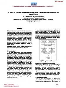
Practical signals are limited both in time (or space in case of images) and frequency. Timelimited signals can be represented efficiently using a set of block functions (Dirac delta functions for infinitesimal small blocks). But block signals are not limited in frequency. Band-limited signals can be represented efficiently using a Fourier basis, but sines and cosines are not limited in time. Wavelets are a compromise between these worlds; wavelet functions can be neatly held finite in both time and frequency domains. Therefore they can be used to approximate data with discontinuities or spikes or detect the contours of objects in images [6]. In Wavelet Transform, temporal analysis is performed by applying concentrated (high frequency) versions of the mother wavelet on the input data, while frequency analysis is done using the dilated (low frequency) versions of the mother wavelet. Figure 2-3-left depicts translations of a prototype wavelet while Figure 2-3-right shows dilations of it.

2.2.2 Multi-Resolution Analysis The main difference between Discrete Wavelet Transform and Windowed Fourier Transform is that DWT analyzes the data in different scales or resolutions. This principle is called Multi Resolution Analysis (MRA). MRA analyzes the signal at different frequencies with different (time) resolutions. It is designed to give good time resolution at high frequencies, and good frequency resolution at low frequencies. Figure 2-4-left and Figure 2-4-right compare the time-frequency plane of Discrete Wavelet Transform against that of Windowed Fourier Transform. It can be seen from Figure 2-4-right that in time-frequency plane of DWT the area covered by individual blocks is equal but that the time-frequency ratio is different. Simply stated, this means that we look at the data in different window sizes. When analyzing with a large window, we notice the global behavior of the data and, conversely, when analyzing with a small window, we focus on the local features of the signal. This makes Wavelet Transform an interesting and useful tool for image processing and image compression [7]. Multi resolution decomposition of a signal into its coarse and detailed components is useful for data compression, feature extraction and de-noising. In terms of data compression this allows us to represent large smooth areas with a few coefficients, which results to superior objective and subjective performance. In the case of image compression, Wavelet Transform matches well to the psycho-visual models; compression systems based oh the Wavelet Transform yield perceptual quality superior to other models at medium and high compression ratios. Furthermore, the multi-resolution nature of the Wavelet Transform enables easy browsing of image databases. This means that the user may decompose only the coarsest scale representation of an image to decide whether he or she wants to examine it at a finer resolution.

Figure 2-3:

Translations (left) and dilations (right) of a prototype wavelet


7

Figure 2-4:

Time-frequency plane of Discrete Wavelet Transform (left) and Fourier Transform (right)

2.2.3 Properties of wavelets A number of issues are important in designing wavelet functions. This section explains these issues and their effects for image compression applications. Smoothness: It is important that wavelet functions is reasonably smooth. If the wavelets possess discontinuities or strong singularities, coefficient quantization errors will cause these discontinuities and singularities to appear in decoded images. Such artifacts are visually highly objectionable, particularly in smooth regions of images. Approximation accuracy: Accuracy of approximation is another important design criterion that has arisen from wavelet framework. A remarkable fact about wavelets is that it allows constructing smooth, compactly supported bases that can exactly reproduce any polynomial up to a given degree. If a continuous-valued function f(x) is locally equal to a polynomial, we can exactly reproduce that portion of f(x) with just a few wavelet coefficients. The degree of the polynomials that can be exactly reproduced is determined by the number of vanishing moments of the dual wavelet. The dual wavelet has N vanishing moments provided that

∫ x ψ ( x)dx = 0 for k = 0 … N-1 k

~

(Equation 2-7)

Compactly supported bases for L2 for which the dual wavelet has N vanishing moments can locally reproduce polynomials of degree N – 1 [5]. Size of the support of wavelets: The size of the support of the wavelet basis is another important design criterion. Suppose that the function f(x) we are transforming behaves as a polynomial of degree N - 1 in some regions. Assume further that we use a dual wavelet that has N vanishing moments. Then any basis function for which the corresponding dual function lies entirely in the region in which f(x) acts as a polynomial, will have a zero coefficient. The smaller the support of the dual wavelet is, the higher the probability that f(x) behaves as a polynomial and consequently the more zero coefficients we will obtain. More importantly, edges produce large wavelet coefficients. The larger the support is, the more likely it is to overlap an edge. Hence it is important to have wavelets with reasonably small support. There is a trade-off between wavelet support and the regularity and accuracy of approximation. Wavelets with short support have strong constraints on their regularity and


8

accuracy of approximation. But as the support increases, they can be made to have higher degrees of smoothness and numbers of vanishing moments.

2.2.4 Advantages of using wavelets Wavelet Transform have several advantages. Here we list a number of these in regard to image compression and processing. •

One of the main features of Wavelet Transform, which is important for data compression and image processing applications, is its good decorrelating behavior.

•

Wavelets are localized in both the space (time) and scale (frequency) domains. Hence they can easily detect local features in a signal.

•

Wavelets are based on multi-resolution analysis. A wavelet decomposition allows to analyze a signal at different resolution levels (scales), which results in superior objective and subjective performance

•

Wavelets are smooth, which can be characterized by their number of vanishing moments. The higher the number of vanishing moments, the better smooth signals can be approximated with the wavelet basis. A function f defined on the interval [a,b] has N vanishing moments if: b

∫ f ( x) x dx = 0 i

for i= 0,1,….,N-1

(Equation 2-8)

a

•

Fast and stable algorithms are available to calculate the Discrete Wavelet Transform and its inverse. Like FFT, the Discrete Wavelet Transform can be factored into a few sparse matrices using self-similarity properties. This results in an algorithm that requires only order of n operations to transform a data series with length n. this is called Fast DWT of Mallat and Daubechies.

2.3 Conclusions In this chapter we had a concise review of the necessary theoretical background for understanding the Wavelet Transform. We gave the definition of the Wavelet Transform, followed by the Discrete Wavelet Transform. Next, multi-resolution analysis was introduced and subsequently we discussed the properties and advantages of the Wavelet Transform. There are different ways to implement the Wavelet Transform; for instance filter bank implementation or the Lifting scheme. The following chapter explains the Lifting scheme in details, as the proposed design is based on that.


9

3 Chapter 3: Lifting Scheme

W

avelets based on dilations and translations of a mother wavelet are referred to as first generation wavelets or classical wavelets. Second generation wavelets, i.e., wavelets which are not necessarily translations and dilations of one function, are much more flexible and can be used to define wavelet bases for bound intervals, irregular sample grids or even for solving equations or analyzing data on curves or surfaces. Second generation wavelets retain the powerful properties of first generation wavelets, like fast transform, localization and good approximation. Lifting scheme is a rather new method for constructing wavelets. The main difference with the classical constructions is that it is does not rely on the Fourier transform. In this way, Lifting can be used to construct second generation wavelets Lifting scheme [2] can in addition, efficiently implement classical wavelet transforms. Existing classical wavelets can be implemented with Lifting Scheme by factorization them into Lifting steps [8]. The basic idea behind the Lifting Scheme is very simple; we try to use the correlation in the data to remove redundancy. To this end, we first split the data into two sets (Split phase): the odd samples and the even samples (see Figure 3-1). If the samples are indexed beginning with 0 (the first sample is the 0th sample), the even set comprises all the samples with an even index and the odd set contains all the samples with an odd index. Because of the assumed smoothness of the data, we predict that the odd samples have a value that is closely related to their neighboring even samples. We use N even samples to predict the value of a neighboring odd value(Predict phase). With a good prediction method, the chance is high that the original odd sample is in the same range as its prediction. We calculate the difference between the odd sample and its prediction and replace the odd sample with this difference. As long as the signal is highly correlated, the newly calculated odd samples will be on the average smaller than the original one and can be represented with fewer bits. The odd half of the signal is now transformed. To transform the other half, we will have to apply the predict step on the even half as well. Because the even half is merely a sub-sampled version of the original signal, it has lost some properties that we might want to preserve. In case of images for instance, we would like to keep the intensity (mean of the samples) constant throughout different levels. The third step (Update phase) updates the even samples using the newly calculated odd samples such that the desired property is preserved. Now the circle is round and we can move to the next level; we apply these three steps repeatedly on the even samples and transform each time half of the even samples, until all samples are transformed. Below we explain these three steps in more detail. Number of samples λ0

Level 0

λ1 λ2

Figure 3-1:

γ1 γ2

Level -1

Level -2

Number of samples in different levels


10

3.1 Split phase Assume that the scheme starts at level 0. We denote the data set as λ0,k where k represents the data element and 0 signifies the iteration level 0. In the first stage, the data set is split into two other sets: the even samples λ−1,k and the odd samples γ −1,k (see Figure 3-2). This is also referred to as the Lazy Wavelet transform because it does not decorrelate the data, but just sub-samples the signal into even and odd samples.

λ-1,k = λ0,2k γ-1,k = λ0,2k+1

(Equation 3-1) (Equation 3-2)

The negative indices are used according to the convention that the smaller the data set, the smaller the index. γ j,k λ j+1,k Split

Update Predict

λ j,k

Figure 3-2:

The Lifting Scheme, forward transform: Split, Predict and Update phases

3.2 Predict phase or dual Lifting The next step is to use the even set λ−1,k to predict the odd set γ −1,k using some prediction function P, which is independent of the data. The prediction will be Prediction = P ( λ−1,k )

(Equation 3-3)

The more correlation present in the original data, the closer the predicted value will be to the original γ −1,k . Now, the odd set γ −1,k will be replaced by the difference between itself and its predicted value. Thus,

γ −1,k = λ-1,k − P ( λ−1,k )

(Equation 3-4)

Different functions can be used for prediction of odd samples. The easiest choice is to predict that an odd sample is just equal to its neighboring even sample. This prediction method is result to the Haar wavelet. Obviously this is an easy but not realistic choice, as there is no reason why the odd samples should be the equal to the even ones. Another option is to predict that an odd sample γ −1,k is equal to the average of the neighboring even samples at its left end right side λ−1,k , λ0, k +1 .

γ −1,k := λ-1,k −

1 ( λ−1,k + λ0, k +1 ) 2


(Equation 3-5)

11

In other words, we assume that the data has a piecewise linear behavior over intervals of length 2. If the original signal complies with this model, all wavelet coefficients ( γ −1,k , ∀ k) will be zero. In other words, the wavelet coefficients measure to which extent the original signal fails to be linear. In terms of frequency content, the wavelet coefficients capture the high frequencies present in the original signal. The prediction does not necessarily have to be linear. We could try to find the failure to be cubic and any other higher order. This introduces the concept of interpolating subdivision. We use some value N to denote the order of the subdivision (interpolation) scheme. For instance, to find a piecewise linear approximation, we use N equal to 2. To find a cubic approximation N should be equal to 4. It can be seen that N is important because it sets the smoothness of the interpolating function used to find the wavelet coefficients (high frequencies). This function is referred to as the dual wavele. Thus the number of dual vanishing moments defines the degree of the polynomials that can be predicted by the dual wavelet. Figure 3-3-left illustrates linear interpolation (N=2), where one even sample at each side is used for predicting the odd sample, while Figure 3-3-right depicts cubic interpolation (N=4), where two even samples at each side are used for prediction. See [2] for more information on how to calculate the filters.

Figure 3-3:

Examples of different prediction functions. Left: Piecewise linear prediction, N=2, right: Cubic polynomial interpolation, N=4

3.3 Update phase or primal Lifting By iterating the predict step on the λj,k outputs of each level for lets say n times, we can convert all the samples, except N coarsest level coefficients λ-n,k, to their corresponding wavelet coefficients. These last N coarsest coefficients are N samples from the original data and form the smallest version of the original signal. This introduces considerable aliasing. We would like some global properties of the original data set to be maintained in the smaller versions λj,k. for example in the case of images we would like the smaller images to have the same overall brightness, i.e. the same average pixel value. Therefore, we would the last values to be the average of all the pixel values in the original image. This problem can be solved by introducing a third stage: the update stage. In this stage the coefficients λ−1,k are lifted with the help of the neighboring wavelet coefficients γ s, so that a certain scalar quantity Q, e.g. the mean, is preserved.


12

Q(λ-1,k) = Q(λ0,k)

(Equation 3-6)

A new operator U is introduced that ensures the preservation of this quality. Operator U uses

~

a wavelet coefficient of the current level (γj,k) to update N even samples of the same level

~

(λj,k). This preserves N − 1 moments of the lambdas.

λ−1,k := λ−1,k + U( γ −1,k )

(Equation 3-7)

~

This is referred to as primal lifting. N is also called number of real vanishing moments. The

~

higher N , the less aliasing effect will exist in the resulting transform.

3.4 The inverse transform One of the great advantages of the lifting scheme realization of a wavelet transform is that it decomposes the wavelet filters into extremely simple elementary steps, and each of these steps is easily invertible. As a result, the inverse wavelet transform can always be obtained immediately from the forward transform. The inversion rules are trivial: revert the order of the operations, invert the signs in the lifting steps, and replace the splitting step by a merging step. Here follows a summery the steps to be taken for both forward and inverse transform. γj,k Update Predict

Merge

λj+1,k

λj,k

Figure 3-4:

The lifting Scheme, inverse transform: Update, Predict and Merge stages

Forward transform: 1- Split phase:

λ j,k = λ j+1,2k γ j,k = λ j+1,2k+1

2- Predict phase

γj,k = γj,k – P(λj,k)

3- Update phase

λj,k = λj,k + U(γj,k)

Inverse transform: 1- Update phase

λj,k = λj,k – U(γj,k)

2- Predict phase

γj,k = γj,k + P(λj,k)

3- Merge phase:

λ j+1,2k = λ j,k λ j+1,2k+1 = γ j,k


13

3.5 Integer-to-integer transform Integer arithmetic is generally much faster than floating-point arithmetic. Furthermore, integer numbers are more efficient to encode and take less space to store. As a consequence, we prefer to deal with integer numbers and integer arithmetic rather than floating-point. In many applications, especially in image processing, the input data consists of integer samples. Wavelet coefficients, on the contrary, are floating point values. Thus since the filter coefficients are floating-point numbers, even if the input data is integer applying the Lifting and Update steps on the data will result in floating-point numbers. Fortunately the Lifting Scheme can be easily modified to map integers to integers, which is in addition fully reversible and thus allows a perfect reconstruction of the original image. This can be is done by adding scaling and rounding operations at the expense of introducing a nonlinearity in the transform. First, the Predict and Update filter coefficients are scaled up and rounded to integers. As both the data and the filter coefficients are integer values, integer arithmetic can now be used. Rounding of the filter coefficients introduces some error, denoted as E below. Forward transform: γj,k,forward, = γj,k,original – {P(λj,k) + E} λj,k,forward = λj,k,original + {U(γj,k) + E}


The introduced error E is fully deterministic, i.e. while calculating the inverse transform, we introduce exactly the same error. Equations below show that the original values are exactly reproducible irrespective of the rounding error. This means a perfect reconstruction of the original image, provided that the transform coefficients are not quantized. Obviously, quantization will still cause distortion in the reconstructed image. Inverse transform: = γj,k,forward + {P(λj,k) + E} γj,k = γj,k,original – {P(λj,k) + E} + {P(λj,k) + E} = γj,k,original

λj,k

= λj,k,forward – {U(γj,k) + E} = λj,k,original + {U(γj,k) + E} – {U(γj,k) + E} = λj,k,original

3.6 Boundary treatment Real world signals are limited in time (space), i.e. they do not extend to infinity. Filter bank algorithms assume, however, that the signal is infinitely long. There a number of ways to deal with this problem. One could for instance extend the signal with zeros (zero padding). In this case the number of coefficients of the transformed signal will be obviously more than the original signal. Furthermore, as signals do not generally converge to zero towards the ends, extending the signal with zeros can lead to coefficients with large values, which leads to significant coding inefficiencies. Truncating the number of coefficients to the number of samples of the original signal, or quantization errors of coefficients with large values will significantly distort the reconstructed image. Another option is make the signal periodic, i.e. to repeat the signal at its ends (Figure 3-5-b). As the values at the left and right ends of the signal are not necessarily the same, discontinuity


14

will appear at signal ends and as a result, a similar problem can arise as mentioned with zero padding. For symmetrical wavelets, an effective strategy for handling boundaries is to extend the image via reflection. Such an extension preserves continuity at the boundaries and usually leads to much smaller wavelet coefficients than if discontinuities were present at the boundaries (Figure 3-5-c). An alternative approach is to modify the filter near the boundaries. In this method, not the signal, but the filter is modified around the boundaries to construct boundary filters that preserve filter’s orthogonality [9] [10]. The lifting scheme [11] provides a related method for handling filtering near the boundaries.

Figure 3-5: Examples of signal extension a: A finite signal

b: Periodic extension

c: Symmetric extension

3.7 Advantages of the Lifting scheme Summarized, the lifting scheme has the following immediate advantages, when compared to the classical filter bank algorithm: 1. Lifting leads to a speedup when compared to the classic implementation. Classical wavelet transform has a complexity of order n, where n is the number of samples. For long filters, Lifting Scheme speeds up the transform with another factor of two. Hence it is also referred to as fast lifting wavelet transform (FLWT). 2. All operations within lifting scheme can be done entirely parallel while the only sequential part is the order of lifting operations. 3. Lifting can be done in-place. An auxiliary memory is not needed since it does not need other samples than the output of the previous lifting step. At every summation point the old stream is replaced by the new one at every summation point. 4. Lifting Scheme allows integer-to-integer transform while keeping a perfect reconstruction of the original data set. This is important for hardware implementation and lossless image coding. 5. Lifting allows adaptive wavelet transforms. This means that the analysis of a function can start from the coarsest level, followed by finer levels by refining in the areas of interest.


15

3.8 Conclusions In this chapter we focused on the Lifting scheme implementation of the Wavelet Transform. We saw that the Lifting scheme uses three simple steps to calculate the wavelet coefficients, namely the Split, Predict and Update phase. We discussed these three steps and explained how the inverse transform can easily be calculated in a similar way. Furthermore, we noticed that the Lifting scheme is not sensitive to deterministic rounding errors that occur in finite precision calculations and, therefore, is suitable for integer calculation. We also discussed how boundary issues, rising in finite length signals, can be treated by using adaptive filters in the Lifting scheme. Conclusively, some nice properties of the Lifting Scheme were listed. Chapter 4 proceeds describing the Lifting scheme by explaining how the Lifting based Discrete Wavelet Transform is applied to 1-D and 2-D signals in the Liftpack software [2].


16

4 Chapter 4: Software implementation: Liftpack

L

iftpack is a software package written in C for fast calculation of 2-D bi-orthogonal Wavelet Transforms using the Lifting Scheme (Fast Lifted Wavelet Transform or FLWT). Originally, the software uses floating-point arithmetic for the transform. For this project we modified the software to use integer arithmetic for higher efficiency. We used this software as a benchmark to see how much the transform would be improved if it would be implemented in hardware. For performance comparison, the software was executed using a simulator, called Sim-outorder, which simulates a MIPS-based processor and the performance were compared to that of the hardware implementation of the transform. In this chapter we discuss the transform, as implemented in Liftpack for a better understanding of the structure of the hardware implementation.

4.1 Attributes of the transform Before going to the implementation details, we give a list of the most important parameters that are used in the scheme. o o o o o o o o

Filter coefficients matrix size: (N/2 + 1)*N ~ Number of iterations n = log 2 (( L − 1) /( N max − 1)) , where Nmax=max(N, N )

Number of coefficients at current level C = L / s  ,where s is the step size between similar coefficients at current level Number of γ s at current level: nG = C / 2

Number of λ s at current leveln: nL = C - nG Number of cases where γ s on left < γ s on right: N/2 - 1 Number of cases where γ s on left = γ s on right: nG – N + 1 + odd(C), where odd(C) is equal to 1 if C is odd and equal to 0 if C is even Number of cases where γ s on left > γ s on right: N/2 – odd(C)

4.2 Predict and update filters In [2] it is explained how to calculate the filter coefficients for the Predict step (filter coefficients) and the Update step (Lifting coefficients). Both sets of coefficients are stored in matrices. For the filter coefficients, the matrix consists of N/2 + 1 rows of each N columns, so in total it has (N/2 + 1)*N entries, where N is the number of vanishing moments. Table 4-1 shows the filter coefficients for N=2, while Table 4-2 illustrates the filter coefficients in case N=4. These tables contain N+1 rows; one row for each interpolating case. Due to the symmetry in the in the rows, they can be stored in only N/2 +1 rows.

~

~

For lifting coefficients, the matrix consists of n * G * N rows, where N is the number of real vanishing moments, n is the maximum number of iterations and G is the number of γ

~

~

coefficients. Thus a separate set of N coefficients is used for each γ to update N λs. In


17

additions, different iteration levels use different sets of lifting coefficients. Table 4-3 and

~

~

Table 4-4 depict the lifting coefficients for N =2 and N =4, respectively. In both cases the signal length is 16 (L=16).

Table 4-1:

Filter coefficients for N=2

Table 4-2:

Filter coefficients for N=4

Table 4-3:

Lifting coefficients for N =2 and L=16

Table 4-4:

Lifting coefficients for N =4 and L=16

~


~

18

4.3 One-dimensional transform As mentioned before, one way of solving the boundary problems is to adapt the filters such that the filter orthogonality is preserved near the boundaries. This means that near the boundaries, the filter coefficients are different than elsewhere in the signal. We say that near the boundaries the filter is affected by the boundaries and elsewhere it is not affected. [2] shows how the filters should be calculated. For the predict phase, this means that a different set of filter coefficients is used for each affected γ. An affected γ is one that is near enough to the edge to be affected by the boundary, i.e. there will not be enough λs to predict the γ. In this case we use the set of N λs near the edge and use the corresponding set of filter coefficients (predict filter) to predict the γ. A similar story holds for the update phase; near the boundaries, when there are not enough λs, ~ we use the set of N λs near the edge. However, the lifting filter (update filter) contains a separate set of coefficients for each γ, thus also a different set of coefficients for each notaffected λs. We use two examples to illustrate how the 1-D transform is accomplished in the Lifting Scheme. The example described in Section 4.3.1 explains how split, predict and update phases are applied to one iteration of a 1-D signal. The example explained in Section 4.3.2 shows how the different iterations of a 1-D signal are performed

4.3.1 Example of 1-D transform: one iteration Considering we have a signal with length 12, we illustrate the calculations for the first level (level 0) of the forward transform on this signal, assuming values 4 and 4 for the number of

~

dual and real vanishing moments, respectively (L=12, N=4, N =4). Here we concentrate on the transform of just one iteration level. Fi,j i=0 i=1 i=2 i=3 i=4 Table 4-5:

j=0 2.1875 0.3125 -0.0625 0.0625 -0.3125

j=1 -2.1875 0.9375 0.5625 -0.3125 1.3125

J=2 1.3125 -0.3125 0.5625 0.9375 -2.1875

J=3 -0.3125 0.0625 -0.0625 0.3125 2.1875

Filter coefficients Fi,j for N=4

The last 2 rows in Table 4-5 are the mirror of the first 2 rows (N/2 + 1 rows of storage area is actually enough for this table). Here all rows are mentioned for clarity.

~

With L=12 and N =4 there will be just one iteration level. The lifting coefficients Li,j then yields: Li,j i=0 i=1 i=2 i=3 i=4 i=5 Table 4-6:

j=0 0.2334861 -0.1823953 0.0107128 -1.9632622 0.6300105 -0.6486542

j=1 0.3348973 0.3778513 0.3362593 3.0021775 -0.9416877 0.9603294

J=2 -0.0540972 0.1461731 0.1458116 -0.2104293 0.4528739 -0.2663926

J=3 -0.0086477 0.0280710 0.0553489 -1.5663428 0.8391388 -0.2796945

~

Lifting coefficients Li,j for N =4


19

Here follows the calculations for the γ coefficients of the first level (predict phase). Figure 4-1 illustrates this graphically. Notice how boundaries are handled here; the left-affected γ, (γ-1,0) uses the left most 4 λ s. These are also used for the first not-affected γ. The same way, the two right-affected γ s (γ-1,4 and γ-1,5) use the 4 λ s at the right side. These λs are also used for the last not-affected γ. Split: γ-1,0 = λ0,1 γ-1,1 = λ0,3 γ-1,2 = λ0,5 γ-1,3 = λ0,7 γ-1,4 = λ0,9 γ-1,5 = λ0,11

λ-1,0 = λ0,0 λ-1,1 = λ0,2 λ-1,2 = λ0,4 λ-1,3 = λ0,6 λ-1,4 = λ0,8 λ-1,5 = λ0,10 Predict: (L: Left-affected, N: Not-affected, R: Right-affected) γ-1,0 -= (λ0,0 . F1,0) + (λ0,2 . F1,1) + (λ0,4 . F1,2) + (λ0,6 . F1,3) (L) γ-1,1 -= (λ0,0 . F2,0) + (λ0,2 . F2,1) + (λ0,4 . F2,2) + (λ0,6 . F2,3) (N) γ-1,2 -= (λ0,2 . F2,0) + (λ0,4 . F2,1) + (λ0,6 . F2,2) + (λ0,8 . F2,3) (N) γ-1,3 -= (λ0,4 . F2,0) + (λ0,6 . F2,1) + (λ0,8 . F2,2) + (λ0,10 . F2,3) (N) γ-1,4 -= (λ0,4 . F3,0) + (λ0,6 . F3,1) + (λ0,8 . F3,2) + (λ0,10 . F3,3) (R) γ-1,5 -= (λ0,4 . F4,0) + (λ0,6 . F4,1) + (λ0,8 . F4,2) + (λ0,10 . F4,3) (R) Now with the newly calculate γ s we update the λ s (update phase). These calculations are listed below. Figure 4-2 illustrates this graphically. The boundaries in update phase are handled in a similar way to the predict phase; the left-affected γ (γ-1,0) updates the left most 4 λ s. These λ s are also used for the first not-affected γ. The same way, the two right-affected γ s (γ-1,4 and γ-1,5) update the 4 λ s at the right side. These λ s are also updated by the last notaffected γ. Update: (L: Left-affected, N: Not-affected, R: Right-affected) λ-1,0 += γ-1,0 . L0,0 λ-1,1 += γ-1,0 . L0,1 λ-1,2 += γ-1,0 . L0,2 λ-1,0 += γ-1,1 . L1,0 λ-1,1 += γ-1,1 . L1,1 λ-1,2 += γ-1,1 . L1,2 λ-1,1 += γ-1,2 . L2,0 λ-1,2 += γ-1,2 . L2,1 λ-1,3 += γ-1,2 . L2,2 λ-1,2 += γ-1,3 . L3,0 λ-1,3 += γ-1,3 . L3,1 λ-1,4 += γ-1,3 . L3,2 λ-1,2 += γ-1,4 . L4,0 λ-1,3 += γ-1,4 . L4,1 λ-1,4 += γ-1,4 . L4,2 λ-1,2 += γ-1,5 . L5,0 λ-1,3 += γ-1,5 . L5,1 λ-1,4 += γ-1,5 . L5,2


λ-1,3 += γ-1,0 . L0,3 λ-1,3 += γ-1,1 . L1,3 λ-1,4 += γ-1,2 . L2,3 λ-1,5 += γ-1,3 . L3,3 λ-1,5 += γ-1,4 . L4,3 λ-1,5 += γ-1,5 . L5,3

(L) (N) (N) (N) (R) (R)

20

Figure 4-1:

An example of calculations of Predict phase, L=12,N=4

Figure 4-2:

An example of calculations of Update phase L=12, N~ =4


21

4.3.2 Example of 1-D transform: more iterations In the previous example we explained the algorithm for one iteration level of a 1-D signal. Here we proceed by describing the 1-D algorithm for more levels. We would like to see how the transform for different iteration levels would look like for a signal with length 32 if we choose values 4 and 4 for the number of dual and real vanishing moments, respectively (L=32, N=4, N~ =4). From Section 4.1 we calculate number of iterations n as log 2 (( L − 1) /( N max − 1)) = 3. For these three iterations levels we calculate the following parameters: 0 32 16 16 1 13 2

Iteration level Number of coefficients at current level C Number of γ s at current level nG Number of λ s at current level nL Number of cases where γ s on left < γ s on right Number of cases where γ s on left Number of cases where γ s on left > γ s on right

1 16 8 8 1 5 2

2 8 4 4 1 1 2

1-D transform parameters for different iterations (L=32, N=4, N~ =4)

Table 4-7:

Figure 4-3 demonstrates these 3 levels. Each block performs split, predict and update phases on its input. This means that the half of the input samples of each block are predicted, marked by ‘x’ in the figure at each level. After 3 iterations, all the samples are transformed and what remains is N λ s which form the smallest sub-sample of the original signal.

γ

λ

γ

λ

γ

λ

γ

λ

γ

λ

γ

λ

γ

λ

γ

λ

γ

λ

γ

λ

γ

λ

γ

λ

γ

λ

γ

λ

γ

λ

γ

Level 0

Level 1

Level 2

Figure 4-3:

Three level decomposition of a 1-D signal with length12 (L=12, N=4, N~ =4)

4.4 Two-dimensional transform The 2-D transform is performed by applying the 1-D transform algorithm consecutively on the rows and columns of a 2-D signal. Considering an image with dimensions X and Y and denoting nX and nY as desired number of iterations in x and y direction, respectively (see Section 4.1), the forward 2-D transform algorithm is as follows: For the forward 2-D transform, we begin with iteration level 0 as current level (CL). The 1-D forward transform is first applied to all the rows, and then to all the columns. Subsequently we move to the next iteration level and repeat the two steps above, and so on, until all the iteration levels are accomplished. If the image is not square (X and Y not equal), the number


22

of iterations in x and y direction can be different. As a consequence applying the 1-D transform on rows or columns might have to be skipped after a certain iteration level in the above algorithm. For the inverse transform, the inverse 1-D transform is applied exactly in the opposite order. Flowcharts below illustrate the 2-D forward and inverse algorithm. In appendix B the 1-D and the 2-D forward and inverse transform are explained in pseudo code format. 2-D forward transform

2-D inverse transform

CL = 0

CL = max(N,Ntilde)

nX < CL

No

Yes

forward 1-D transform on rows

No

nY >= CL

No

nY < CL

Yes

forward 1-D transform on columns

inverse 1-D transform on columns

Yes

inverse 1-D transform on rows

No

nX >= CL

No

No

CL = CL + 1

CL = CL - 1

CL< max(N,Ntilde)

CL > 0

Yes

Yes

stop

stop

Figure 4-4:

Yes

Flow chart of the 2-D forward and inverse transform

4.5 Example: 2-D transform Here we consider the steps taken for in the 2-D transform of an image with dimensions 128 and 32 in x and y directions respectively. As described in Section 4.1, we calculate 5 and 3 for the number of iterations in x and y directions, respectively (N=4, N~ =4). The steps to be taken for the 2-D transform of this image is illustrated in Table 4-8 (the split step is not mentioned). As can be seen, in the forward transform after step 14 and 16, and in the inverse transform before steps 1 and 3, the 1-D transform on the columns is skipped.


23

Forward Transform 1 2 3 4

Predict Update Predict Update

Rows Rows Columns Columns

Level 0 Level 0 Level 0 Level 0

5 6 7 8



9 10 11 12


Inverse Transform

1 2

Update Predict

Rows Rows

Level 4 Level 4


3 4

Update Predict

Rows Rows

Level 3 Level 3



5 6 7 8

Update Predict Update Predict

Columns Columns Rows Rows


13 Predict 14 Update -

Rows Rows -

Level 3 Level 3 -

9 10 11 12




15 Predict 16 Update -

Rows Rows -

Level 4 Level 4 -

13 14 15 16




Table 4-8:

Steps taken to transform a 2-D signal (Lx=128, Ly=32, N=4, N~ =4)

4.6 Conclusions In this chapter we described the Lifting scheme implementation of the Wavelet Transform from as implemented in Liftpack software. We explained how some important parameters are calculated and we gave examples of predict and update filters. Subsequently, examples were given for the 1-D and 2-D transform, which are essential for understanding the organization of the hardware module. Chapter 5 uses the examples given here, delves into the structure of the hardware design and describes them in detail.


24

5 Chapter 5: Hardware implementation

I

n the previous chapter, the algorithm of the Lifting-based Discrete Wavelet Transform (FLWT) was explained in detail. The Lifting Scheme is indeed a fast implementation of the DWT. However, the performance of the pure software implementation of this algorithm on general-purpose processors (GPP) is known to be the performance bottleneck for practical applications. The objective of this project was to improve the performance of the DWT for image compression applications by performing parts of, or the entire transform in a dedicated hardware unit. The unit is meant to be integrated in custom-computing machine (CCM), as a reconfigurable functional unit. This means that the unit will co-exist with a general-purpose processor and will execute wavelet transform operations in hardware, upon occurrence. In this chapter, we investigate the restrictions of the software implementation and introduce hardware schemes to overcome these restrictions. We follow a bottom-up approach to describe the design i.e., we start from the lowest level and build up the structure of the design gradually.

5.1 Architectural considerations General-purpose processors have the typical property of executing programs in a sequential manner. Even though modern superscalar processors can execute more than one instruction at a time, this feature is limited to extracting independent instructions in a rather small instruction window. Therefore, if parallel operations exceed the instruction window, the parallelism will not be detected and utilized. In the hardware domain, in contrast, the design can be implemented such that the existing parallelism in the algorithm is exploited methodically. Moreover the amount of parallelism introduced in general-purpose processors is limited to a few functional units, while in the hardware domain, when a large reconfigurable hardware resource is available, multiple parallel operating functional units can be instantiated, which can lead to performance improvement. Another limitation of general-purpose processors is their comparatively small number of registers. Due to the lack of registers, reusable data residing currently in the registers will be overwritten and have to be read from the memory again when required in the future. This obviously deteriorates the performance, as a memory access is significantly slower than a register access. In hardware, the amount of data storage elements can be substantially larger, and can hold the needed data for fast future access. A thorough investigation of the FLWT algorithm shows a considerable amount of operations that can be performed in parallel. Furthermore, a smart design can significantly reduce the amount of data transfer to and from the image memory by buffering data that once has been read from the memory. Additionally, Xilinx Virtex II FPGA platform provides true dual port internal RAM blocks, which can be taken advantage of. The proposed hardware introduces the following features which lead to a noticeable performance rise of the hardware implementation, even though the hardware operates at a clock frequency of 50MHz, against an assumed microprocessor clock frequency of 1GHz (20 times lower).


25

-

Parallel operations in predicting one γ Parallel operations in updating λs from one γ Reusing data in predicting one γ Reusing data in updating λs from one γ Parallel execution of 1-D predict and update phases Reusing data in 1-D predict and update phases Increasing data access rate using Xilinx dual port RAM Increasing data access rate by performing two data accesses in one cycle (RAM clock frequency = 2*system clock frequency)

Following sections address each of these issues in detail.

5.1.1 Accelerating the predict stage We use the example discussed in Section 4.3.1 to explain the features of the hardware design. In this example, number of dual vanishing moments (N) is equal to 4, but the concepts described below can be applied to any value of N. Figure 4-1 demonstrates the algorithm for the 1-D predict phase and the calculations for a single γ are illustrated in Figure 5-1. γj-1

λj,k+2 λj,k Fi,0

λj,k+4 λj,k+6

Fi,2

Fi,1

-+ - -

Fi,3

γj-1

Figure 5-1:

Predicting one γ from 4 λ s in forward transform

γ j −1 − = (λ j ,k .Fi ,0 ) + (λ j ,k + 2 .Fi ,1 ) + (λ j ,k + 4 .Fi , 2 ) + (λ j ,k + 6 .Fi ,3 )

(Equation 5-1)

In a general-purpose processor this will be translated to for n=0 to N { γj-1,n += λi * Li,n } which results in 16 memory access: 4 times (read λ, read lifting coefficients, read γ, write γ)) 4 multiplications 4 additions/subtractions The hardware implementation can be designed perform do all 8 arithmetic operations in parallel. The problem would be performing all memory accesses in parallel. We break this problem into 4 sub problems: -

Accessing N λs concurrently Accessing N filter coefficients concurrently Reading input γ concurrently Writing back predicted γ concurrently


26

5.1.1.1

Accessing N λs concurrently

The calculation for predicting two consecutive not-affected γ s, as described in Section 4.3 and Figure 4-1, is shown in figure below.

F2,1

F2,2

F2,0

F2,3

γ-1,1 F2,1

F2,2

F2,0

F2,3

γ-1,2

Predicting two consecutive γ s

Figure 5-2:

As can be seen, 3 of the 4 λ s are used in both calculations. For the case of left- or rightaffected γ s, all 4 λ s are common in both calculations. This implies that reading only one λ from the memory will be sufficient to calculate the following γ, if λ s of the preceding calculation are stored in temporary buffers for reuse. This reduces memory reads from N to only one. This idea can be implemented by using a pipeline of N registers for λ inputs. The pipeline is filled in N cycles in the start, after which it can offer parallel access to N λs. Prior to moving towards the next γ, the content of each register is transferred to the adjacent register and the rightmost register (λ3 in Figure 5-3) is read from the memory. λin clock

λ0

λ1

Figure 5-3:

5.1.1.2

clock

λ2

clock

λ3

clock

Pipelining for parallel access to λs

Accessing N filter coefficients in parallel

All not-affected γ s use the same set of 4 filter coefficients for calculation. However, each left- and right-affected γ s uses a separate set of 4 filter coefficients, which means that no data reusability exists in left- and right-affected filter coefficients. Therefore we use 4 separate banks of RAM for the filter coefficients; each corresponding to one λ. This structure allows us to access 4 filter coefficients at the same time (see Figure 5-4).

Predict filter RAM 0

clock address

Figure 5-4:


clock address


clock address


clock address

Using distinct banks of RAM for filter coefficients for parallel access


27

5.1.1.3

Reading input γ concurrently

In the previous section, we explained how 4 memory reads can be reduced to only 1, by using registers to buffer the λ s. However, the input γ also has to be read simultaneously as well (see Figure 5-1). This means that two different locations of the image storage area have to be accessed at the same moment. Fortunately there is a way to tackle this problem. Xilinx Virtex II FPGAs come with embedded real dual port RAM blocks. These RAM blocks feature two separate input/output ports which can be addressed independent from each other. This allows different combinations of two simultaneous memory operations: two reads from two different locations one read from and one write to two different locations two writes to different locations Furthermore, it is possible to read a memory location before writing into it, at the same cycle. Using the internal dual port RAM block of Virtex II FPGA series for picture data, we can access the γ and λ inputs concurrently (see Figure 5-5). Address-A DataOut-A (λ)

DataIn-A

Dual port Picture RAM

Enable-A WriteEnable-A

Address-B DataIn-B Enable -B DataOut-B (γ)

Figure 5-5:

5.1.1.4

WriteEnable -B

Dual port RAM is used for simultaneous access to two values (γ and λ)

Writing back predicted γ concurrently

Reading the γ and λ simultaneously occupies both ports of the dual port picture RAM. Nevertheless, we need to write back one predicted γ at the same hardware cycle if we wish to perform the whole predict operation in one cycle. This problem can be solved if the picture RAM can operate with a frequency two times higher than the rest of the design (see Figure 5-6). The practice shows that this is possible; the design operates at a clock period of 20 ns, while the RAM blocks can operate with a clock period of 3.7 ns. This means that the internal RAM can operate on a much higher frequency than the remainder of the design. If we perform one memory access per half system cycle, in total 4 memory locations can be addressed per system cycle (there are 2 ports and they can be addressed 2 times per cycle). The section on timing (Section 5.3) explains more about this issue. System clock period

System clock

Picture RAM clock

read

Figure 5-6:

write

Picture RAM can be accessed twice per system cycle


28

5.1.1.5

The predict module

Using the techniques explained above, we compose the Predict Module as shown in Figure 5-7. Starting to predict a 1-D signal (a row or a column of the picture), the rightmost register (λ3) is loaded from the picture RAM. In the next 3 cycles the contents of the registers are shifted to their left neighbor, while λ3 keeps on reading the data from the picture RAM. In the meanwhile, the corresponding filter coefficients and γ are ready respectively at predict coefficient and γin inputs of the module for predicting the first γ. The γ will be calculated and saved in the γ register. Now, for calculating the left- and right-affected γ s, the contents of the λ registers are kept unaltered (no shifting) and only the corresponding filter coefficients and γ is read each cycle. For calculating the not-affected γ s, the λ registers are shifted to the left and the corresponding λ3, γ in and filter coefficients are read. In the following we explain a number of other issues deserve to be described. The objective of the predict module is to calculate γ j-1 (see Section 3.5) as

γ j −1 − = (λ j ,k .Fi ,0 ) + (λ j ,k + 2 .Fi ,1 ) + (λ j ,k + 4 .Fi , 2 ) + (λ j ,k + 6 .Fi ,3 )

(Equation 5-2)

Scaling: As the filter coefficients are mostly very small, the finite precision of integer arithmetic causes huge non-linearities. In order to alleviate this effect, we scale up the filter values prior to the calculation and scale back the result afterwards.

γ j −1 − =

(λ j , k .( Fi ,0 .Scale)) + (λ j , k + 2 .( Fi ,1.Scale)) + (λ j , k + 4 .( Fi , 2 .Scale)) + (λ j , k + 6 .( Fi ,3 .Scale)) Scale (Equation 5-3)

In Figure 5-7, the up-scaling of the filter coefficients is not explicitly shown, but the triangle with text 2-PS denotes the down-scaling with a factor 2PS (Predict Scale).

Forward and inverse transform: The predict phase of forward and inverse transform differ just in one operation:

γj,k = γj,k – P(λj,k) γj,k = γj,k + P(λj,k)

forward transform inverse transform

Therefore we introduce a single predict module, which can operate both for forward and inverse transform by selectively adding or subtracting the prediction from the original γ. This is implemented in the predict module (Figure 5-7) by selectively negating the prediction before the last adder for forward transform. Control signal FW/IV indicates whether the module should operate in forward or in inverse mode. Pipelining of the output: Another issue to notice is that the predicted γ is registered at the output. This forms a pipeline for the stages using the γ output and improves the performance by decreasing the total latency.


29



Predict coefficient 0

λ0



clock enable



clock enable

λ1

λ2


clock enable

λ3

λin

λ

clock enable

2-PS

-1 1 0

FW/IV

1

γin

γ

clock

γout

Predict module

Figure 5-7:


Predict module

30

γ

5.1.2 Accelerating the update stage We use the example explained in Section 4.3.1 to explain the features of the hardware design

~

for the update phase. In this example, number of real vanishing moments ( N ) is equal to 4,

~

but the concepts described below hold for any value of N . Figure 4-2 demonstrates the algorithm for the 1-D update phase. Illustration below shows how a single γ is used to update

~ N λ s.

λj-1,k+0

λj-1,k+1 Li,0

λj-1,k+2 Li,1

λj-1,k+3 Li,2

Li,3

γi

λj-1,k+0

Figure 5-8:

λj-1,k+1

λj-1,k+2

λj-1,k+3

Updating 4 λ s from one γ in forward transform

Which is the graphical demonstration of the following equations:

λ-j-1,0 += γ i . Li,0 λ-j-1,1 += γ i . Li,1 λ-j-1,2 += γ i . Li,2 λ-j-1,3 += γ i . Li,3 In a general-purpose processor this will be translated to

~

for n=0 to N { λj-1,n += γi * Li,n } which results to 16 memory access: 4 times (read λ, read lifting coefficient, read γ, write γ)) 4 multiplications 4 additions/subtractions The hardware implementation can be designed to perform all 8 arithmetic operations in parallel. The problem would be performing all memory accesses in parallel. We break this problem into 4 sub problems:

~ ~ Accessing N lifting coefficients concurrently

-

Accessing N λs concurrently

-

Reading input γ concurrently

-

~

Writing back N updated λs concurrently


31

5.1.2.1

~

Accessing N lifting coefficients and input γ concurrently

~

For concurrent access to N lifting coefficients and input γ, we use the same design as

~

described in the predict module (see Sections 5.1.1.2 and 5.1.1.3). Accessing N λs and

~

writing back N updated λs, however, is different than in the predict module and is described in the following.

5.1.2.2

~

~

Accessing N λs and writing back N updated λs concurrently

Comparing Figure 5-1 and Figure 5-8 confirms that the major difference between the predict

~

and the update algorithm is that updating causes N outputs (λs), which have to be written back, while predicting leads to just one output (γout). The dual port picture RAM allows us to write back at most 2 values per system clock cycle, as 2 other memory operations are reserved for reading λ and γ inputs. Furthermore, we would like to use one of these ports for writing back the predicted γ s from the predict module, which leaves us with only one free port and

~ N (4 in this case) λs to store. Can we overcome this problem?

Figure 4-2 consists of 6 separate rows, each corresponding to one γ updating four λs. We denote each row as an stage and distinguish three different categories: 1- All 4 outputs of the stage are used as inputs in the subsequent stage. Examples are rows 1, 4 and 5; all the outputs of stage 1 are used as inputs of stage 2. 2- Except the leftmost output, all the outputs of the stage are used as inputs of the subsequent stage. Examples are rows 2 and 3; the leftmost output of stage 2 has to be written back to the memory and the other 3 are used as inputs of stage 3 i.e. outputs 1,2 and 3 are used as inputs 0,1 and 2 of stage 3. 3- Non of the outputs of the stage are used by other stages. This is the case in the last stage (row 6). In this case all outputs have to be written back into the memory. This observation confirms the following: It can be inferred from Figure 4-2, that if the outputs of each stage are made available for the inputs of the following stage, all stages lead to at most one value to be written back to the memory, except for the last row that produces 4 outputs to be written back. This means that the problem of writing back 4 λs can be reduced to writing back just one λ. The last stage, however, will still need 4 write backs, but this can be done in 4 separate cycles, as no other update operation has to be performed on them. In order to provide all desired functionalities, the design should be adaptable in a number of different configurations. We distinguish four configurations: Fill configuration: Parallel access to N~ λs is desired. However, one port is available for ~ reading λs. To overcome this problem, we introduce a series of N registers and connect them in a pipelined fashion. The pipeline is filled in N~ cycles in the start, after which it can offer

~

parallel access to N λs (see Figure 5-9).


32

Figure 5-9:

Filling the update pipeline for parallel access to λs

In-place configuration: For the last not-affected γ, all left-affected γ s and all right-affected γ

~

s, except the last one, all the outputs (0 to N -1) are fed to the inputs of the next stage (see Figure 5-10).

Figure 5-10:

Providing the inputs of the next stage with the updated λ outputs

Shift configuration: For not-affected γ s (except the last one), the leftmost output (output 0)

~

is available for writing back into the memory, the outputs 1 to N -1 (1 to 3) are used as inputs

~

0 to N -2 (0 to 2) of the subsequent stage, and the rightmost register is loaded with the corresponding λ from the memory (see Figure 5-11).

Figure 5-11:

Shifting the outputs to the next λ register

Empty configuration: For the last right-affected γ, all the outputs should be available for writing back, i.e. the registers have to be emptied. For this case, we use the same configuration as in Fill configuration (see Figure 5-9). With each clock cycle the contents of the λ registers is shifted to the left and can be written back into the memory when they are located in register λ0.


33

5.1.2.3

The update module

The preceding section defined the required functionality of the update module. We propose the structure as shown in Figure 5-12 for the update module. The following explains how control signals set the update module to operate in different configurations. Fill: Starting to update a 1-D signal (a row or a column of the picture), we set the control signal nextλ to 1 and present value 0 at γin input. Which configures the module as depicted in Figure 5-9. Now the rightmost register (λ3) is loaded from the picture RAM. In the next 3 cycles, the contents of the λ registers are shifted to their left neighbor, while λ3 keeps on reading the data from the picture RAM. While filling the last λ, the corresponding filter coefficients and γ for the first update (first left-affected γ) are loaded respectively at the update coefficient and γin inputs of the module. Now all the necessary data for updating with the first left-affected γ are available. The updated λs are calculated and will be waiting at the output of the adders to be stored. In-place: Resetting the control signal nextλ to 0, configures the module as illustrated in Figure 5-10, which transfers the output of the each adder to the same λ register. Shift: Setting the control signal nextλ to 1, configures the module as illustrated in Figure 5-11. Each updated λ (output of the adders) is shifted Empty: this configuration is equal to fill configuration. The only difference is that unlike fill, the values will be written back into the memory, when they are available at λout output. In the following, we explain a number of issues concerning the update module: Concurrent memory access: Similar to the predict module, the update module requires two memory reads per cycle for γin and γin. Also the λout output has to be written back concurrently. We use the same concept as in the predict module to overcome these problems. This means that γin and γin are provided using the dual port RAM concept (see Sections 5.1.1.3 and 5.3). For concurrent write-back of λout output, we use the same structure as in the predict module, i.e. splitting a system clock cycle into two halves and performing one memory operation in each half (see Section 5.1.1.4). Scaling: The objective of the update module is to calculate λ-j-1 (see Section 3.5) as:

λ j −1,k + = γ i .Li ,k

(Equation 5-4)

As the update coefficients are mostly very small, the finite precision of integer arithmetic will cause huge non-linearities. In order to alleviate this effect, we scale up the filter values prior to the calculation and scale back the result afterwards.

λ j −1,k + =

γ i .( Li ,k .Scale) Scale

(Equation 5-5)

In Figure 5-12, the up-scaling of the filter coefficients is not explicitly shown, but the triangles with text 2-US denotes the down-scaling with a factor 2US (Update Scale).

Forward and inverse transform: The update phase of forward and inverse transform differ just in one operation:


34

λj,k = λj,k + U(γj,k) λj,k = λj,k – U(γj,k))

forward transform inverse transform


Therefore we introduce a single update module, which can operate both for forward and inverse transform by selectively adding or subtracting the updates to or from the original λs. This is implemented in the update module (Figure 5-12) by selectively negating the update before the last adder for inverse transform. Control signal FW/IV indicates whether the module should operate in forward or in inverse mode. Pipelining the output: Another issue to notice is that λout is registered at the output. This forms a pipeline for the stages using the λout output and improves the performance by decreasing the total latency.

5.1.3 Accelerating the 1-D transform In Chapters 3 and 4, we introduced the predict and the update modules, which utilize different techniques to accelerate the predict and the update phases separately. Is it possible to have the predict and the update modules to operate simultaneously? This would increase the performance of the transform by a factor of 2. In this chapter we investigate this option and propose an organization, which allows parallel operation of both modules. We distinguish two problems; data dependency and memory bandwidth limitation.

5.1.3.1

Data Dependency

In the software implementation, predict and update phases are executed consecutively. Not surprisingly, this is because of the sequential operation nature of general-purpose processors; the processor is not able to execute both phases simultaneously. In custom design hardware, however, this limitation does not exist; in principle both modules can operate simultaneously. The problem here is the data dependency between the two modules; in forward transform, the update module needs the outputs of the predict module (the predicted γ s) for updating the λs (see Figure 3-2) and in inverse transform, the predict module needs the outputs of the update module (the updated λs) to predict the γ s (see Figure 3-4). Considering Sections 5.1.1 and 5.1.2 on predict and update modules, we notice that except for the beginning and the end of the1-D transform, both predict and update modules create one output each cycle. This means that predict and update modules could operate simultaneously, provided that we wait long enough for the predict module to generates its first output and provided that this output is made available to the update module. Figure 5-13 shows concatenation of the predict and the update modules for forward transform, which allows their parallel operation.


35

Update filter RAM 0

Update filter RAM 1

Update coefficient 0

Update filter RAM 2


Update filter RAM 3



γin

2-US

2-US

2-US

2-US

-1 1

-11

-1 1

-1 1

0

1

FW/IV

0

1

FW/IV

0

1

FW/IV

0

1

FW/IV

λin 0

1

λ0

FW/IV

0

clock λenable

1

λ1

λ

FW/IV

clock λenable

0

1

λ2

FW/IV

clock λenable

0

1

λ3

nextλ

clock λenable

clock

λout

Update module Figure 5-12:


γ

Update module

36

λ

λin

Update module

λout

Figure 5-13:

5.1.3.2

Predict module

γin

γout

λin

γin

Concatenation of predict and update module for forward transform

Memory bandwidth limitation

The technique described in the previous paragraph does not solve all the problem of parallel operation of the predict and update modules. In Section 5.1.1.4 we explained that we can at most have 4 memory operations per system cycle. Concurrent operation of the predict and update modules requires 6 data elements to be accessed: for predict module, λ and γ inputs and γ output, and for update module, λ and γ inputs and λ output. Hence we have too many memory operations per system cycle if we perform all data access directly to the picture RAM. How can we overcome this problem? The three required memory accesses for the predict module, illustrated in Figure 5-13, can be directly accommodated from the picture RAM. Also the output of the update module can be directly written back to the picture RAM (see Section 5.1.1.4). The problem would be providing data to the two inputs of the update module. In the following we will explain how these two inputs can be fed with data, without any access to the picture RAM. Providing data to γ input of the update module: As explained in Section 5.1.3.1 and shown in Figure 5-13, the γ input of the update module can be fed with the output of the predict module. We introduce a First In First Out (FIFO) buffer between the output of predict module and the γ input of the update module to absorb the unequal speed of delivery and consumption rate of data at the beginning and the end of the predict and update phases (see Figure 5-14).

Update module

λout

Figure 5-14:

λin

γin

Predict module

γ FIFO

γout

λin

γin

Using a FIFO buffer to provide the γ input of the update module in forward transform with data

Providing data to λ input of the update module: There is only one more input which has to be provided with data: the λ input of the update module. Considering Figure 3-2, It can be seen that the update phase uses the same λs as the predict phase. However, the predict module reads the λs from the picture RAM at a earlier than required by the update module. As a consequence, it is not possible to fill the λ pipelines of both predict and update modules with the output of the picture RAM. However, placing a FIFO buffer before the λ input of the update module can be the answer to this timing problem. This buffer in fact solves the synchronization problems and allows the update module to reuse the λs once read by the predict module. Figure 5-15 shows how this FIFO is used.


37

Update module

λout

λin

λ

Predict module

FIFO

γin

γ FIFO

γout

λin from picture RAM

γin

to picture RAM

Figure 5-15:

5.1.3.3

Using λ FIFO buffer to provide the λ input of the update module in forward transform

Forward and inverse transforms

The techniques described in Section 5.1.3 and the subsections are based on forward transform. These concepts are, however, also applicable to inverse transform. In case of inverse transform, the two inputs of the update module and its output can be directly addressed by the picture RAM. Also the output of the predict module can be written back into the picture RAM. For λ and γ inputs of the predict module, a similar method as depicted in Figure 5-15 can be used; The predict module needs the output of the update module (updated λs, see Figure 3-4) at its λ input. The output of the update module can be provided to the input of the predict module by introducing a FIFO (λ FIFO in Figure 5-16). The γ input of the predict module, on the other hand, uses the same γ s that are needed for the Update module. We use therefore, a FIFO buffer (γ FIFO in Figure 5-16) to temporarily save the γ s, as they are read from the picture RAM. These values can subsequently be provided to the predict module when they are required. to picture RAM

Predict module

γout

Figure 5-16:

5.1.3.4

λin

γin

λ

FIFO

γ

FIFO

λout

Update module

λin from picture RAM

γin

Using two FIFOs to provide the predict module with the required data in inverse transform

FIFO buffer depth

Assuming the forward transform (Figure 5-15), it can be seen that the λs have to be saved in the λ FIFO from the moment that the first λ is read by the predict module, until the first λ is demanded by the update module. The update module can start reading the λs as soon as the first γ is predicted by the predict module. This takes N+2 cycles, N cycles for filling the predict module’s pipeline, one cycle for the γ output buffer (see Figure 5-7) and one cycle to write the γ in the FIFO. From this moment the update module reads one value out of λ FIFO

~

each cycle, until its pipeline is filled. Now the update module stalls for N 2 + 1 cycles to update the left-affecteds and the first non-affected λs. Thus the λ FIFO buffer should be at

~

~

~

least N + N 2 + 3 deep. The minimum depth for the γ FIFO is N , as it takes N cycles to


38

fill the λ pipeline of the update module after the first γ is predicted by the predict module, during which the γ s should be saved. In case of inverse transform (see Figure 5-16), the γ s have to be saved from the moment that the first γ is read by the update module until the first γ is read by the predict module. The first γ can be read by the predict module as soon as the pipeline of the predict module is filled. The first updated λ is available after all the left-affected and the first non-affected updates are ~ performed by the update module. This leads to N 2 + 2 γ values to be saved (the delay due the λ output buffer is taken into account, see Figure 5-12). From this moment it takes N cycles before the predict module’s pipeline is filled. Therefore, the γ FIFO should be at least ~ N 2 + 2 deep. The depth of the λ FIFO is defined by the number of cycles that the predict module (Figure 5-12) stalls reading λs. This happens while predicting the left-affected and the

~

~

first non-affected γ s. As a result the γ FIFO should be at least N 2 + 1 deep. As N and N are small numbers, typically between 2 and 8, it is convenient to take a common depth for both ~ FIFOs. A safe and yet easily affordable rule of thumb is 2 × ( N + N ) .

5.1.4 Accelerating the 2-D transform In Section 5.1.1.3 we explained how the dual port RAM facility of the Xilinx Virtex II FPGAs helps us increase the performance of the 1-D transform. There are two options for accelerating the DWT: 1-D transform acceleration: In this scheme, one line of the picture (one row or one column) is loaded into the FPGA’s internal RAM, the 1-D transform is performed on the line and the data is written back into the external memory 2-D transform acceleration: In this scheme the data of the whole image is imported into the FPGA’s internal memory, the entire 2-D transform (which is a series of consecutive 1-D transforms) is performed on the data and the transformed image is written back into the external memory. The 1-D scheme requires an internal storage space equal to the length of a line (the maximum of the row length and the column length). For instance CIF picture format (352x288) requires only 352 storage elements of the FPGA’s internal RAM. However, this scheme leads to an excessive amount of data transfer between the hardware module and the external memory. The reason for this is that the 2-D nature and the multiresolution character of the DWT cause multiple operations on the same pixel in different stages. For a picture format of 352x288 pixels, in the 2-D scheme the data for 352*288 = 101376 pixels have into be loaded to the FPGA. In the 1-D scheme, on the contrary, 270270 pixels have to be transferred. In addition, writing the data back into the memory will increase these numbers by another factor of 2. Another major drawback of the 1-D acceleration is the inherent cache misses when memory locations are sparsely accessed. The data of consecutive rows of an image are generally aligned in a linear array in the external memory. This means that accessing the pixels of a row with small strides, as happens in the 1-D transform of the rows in lower iteration levels, does not cause frequent cache misses. However, cache misses will be more frequent when the


39

stride grows, as is the case when performing the 1-D transform on the columns or performing the 1-D transform on the rows in higher iteration levels. We carried out the 1-D and the 2-D accelerated transform on two different picture sizes and compared the results. For a picture format of 352x288, the total data transfer time of the 1-D scheme was 6 times higher than that of the 2-D scheme. In case of a picture size of 720x560, this ratio even increased to a factor of 12. Please refer to Section 6.5 for the details of this experiment. Based on this analysis, and with an eye on the primary objective of this project, which was to accelerate the transform, we chose to implement the 2-D acceleration scheme. However the 1D scheme is as well implemented, since the 1-D transform forms a part of the 2-D transform.

5.2 Design organization In Section 5.1, we described how the performance of the design can be improved, using different techniques. In this section we compose the entire design as illustrate in Figure 5-17 and describe a number of issues with regard to this. In Figure 5-17, the multiplexes before γ FIFO and λ FIFO modules, select which signals will be connected to the input of the FIFOs. The multiplexers before the predict and the update modules choose which signals are fed to the inputs of these modules. These multiplexers choose the correct configuration required for forward or inverse transforms. Prior to performing the transform, it is necessary to import the picture data from an external source (called external RAM in Figure 5-17). When the transform is accomplished, the transformed picture data has to be written back into the external source. Therefore two multiplexers in front of the picture RAM’s datainA and datainB inputs selects whether these inputs should be connected to the external RAM datain or to the outputs of the predict and update modules. These multiplexers allow the picture RAM to receive the data from the external source before starting the transform and write back the data at the to the external memory after the transform is accomplished. As explained in Section 5.1.1.4, the picture RAM is addressed two times per system clock cycle. The two multiplexers in front of picture RAM’s addressA and addressB inputs choose the corresponding address in each half of the system clock. Please refer to Section 5.3 for more details on timing. A multiplexer in front of the update module forces the γ input of the module to zero, if desired. This is required when filling or emptying the pipeline inside the update module (see Fill configuration and Section 5.1.2.3). The predict and update filters are implemented in RAM. This increases the flexibility of the design, as compared to using a ROMs, since the filter data can be dynamically changed, if desired. Using RAM blocks for filters, however, means that they have to be read prior to performing the transform. Nevertheless, this will not decrease the performance of the module, as it has to be done just once after system power-up. Performing subsequent transforms does not require the filter RAM to be re-read. Figure 5-17 depicts the structure of the design. A number of control signals synchronize the data transfer between the modules and implement the 1-D and 2-D transform algorithms as explained in Chapters 3 and 4. These control signals are generated by the control unit (see Figure 5-18).


40

5.3 Timing considerations This section describes the timing of the control signals of the picture RAM in more detail. In Section 5.1.3.2 we described how introducing two FIFO buffers reduces 6 demanded memory accesses per cycle to only 4, two reads and two writes. Using the dual port RAM feature of Xilinx Virtex II FPGA series, 2 memory locations can be accessed simultaneously per cycle. To increase this to 4, we propose to access the picture RAM once per every half of the system cycle. This means that the clock frequency of the picture RAM is twice higher than that of the system. Although the clock frequency of the picture RAM is higher, this signal is not fed to any other logic than the clock input of the picture RAM (see Figure 5-17). Thus RAM clock will not violate the timing constraints of the system. Figure 5-19 illustrates the timing of consecutive reads and writes. As can be seen in Figure 5-19, the first half of the system clock (the HIGH half) is used to write the outputs of the predict and update modules back into the picture RAM (see also Figure 5-17). In the second half of the system clock (the LOW half) both ports of the picture RAM are used to provide λin and γin inputs of the predict module (when doing forward transform) or update module (when doing inverse transform) with data. Figure 5-20 depicts the control logic for the setup described above. A multiplexer selects the correct address for the address input of the picture RAM for each half of the system cycle, i.e. write address for the first half and read address for the second half. The multiplexer is, therefore, driven by system clock signal (see Figure 5-19). It can be seen that the read operations in the second half of system clock always take place (Figure 5-19). However, the data will be written into the picture RAM only if the signal picture_RAM_write_request is high. A combinatorial circuit implements the logic explained above (see combinatorial logic in Figure 5-20).


41

External_RAM_ data_in 0-15 dataIn Update Filter 3

data Out

data Out

data Out

data Out

update_filter_write_enable update_filter_address clock

coeff0

coeff1

coeff2

coeff3

λin

Update module

Clock

FW_IV

update λ_enable

FIFO

dataOut

1

0 1

0

0

Control unit

Figure 5-17:


Predict Filter 0

Predict Filter 1

Predict Filter 2

Predict Filter 3

data Out

data Out

data Out

data Out

γ FIFO

predict_filter_write_enable predict_filter_address clock

coeff0 dataIn

coeff1

coeff2

1

Predict module

dataIn 1

coeff3

0

0 1

λout

1

addressA 0

read_addressA

1

write_addressA

dataInA 1

External_RAM Data_in 0-15

0 Externa_ RAM_ active

FW_IV

γin

γout

clock

Picture RAM

λin

0

FW_IV

dataOut

Update γ in_reset

γin

update nextλ

1

FW_IV

λout

clock RAM_clock reset transform2D_restart FW-IV external_RAM_enable external_RAM_data_in

0

λ

transform2D_done external_RAM_address external_RAM_write_enable external_RAM_enable external_RAM_data_out

dataIn

dataInB 1

γout

0

0

External_RAM data_in 16-31

addressB 0

read_addressB

1

write_addressB clock

picture_RAM_enableA picture_RAM_enableB picture_RAM_write_enableA picture_RAM_write_enableB RAM_clock

Update Filter 2

dataIn

Clock

Update Filter 1

dataIn

FW_IV

Update Filter 0

dataIn

predict_λ_enable

dataIn

λFIFO_Sinit λFIFO_read_enable λFIFO_write_enable clock

dataIn

γFIFO_Sinit γFIFO_read_enable γFIFO_write_enable clock

dataIn

External_RAM_data_out 0-15 External_RAM_data_out 16-31

Top level organization of the hardware unit for acceleration of DWT

42

clock RAM_clock reset transform2D_restart FW-IV external_RAM_enable external_RAM_data_in

Figure 5-18:

transform2D_done external_RAM_address external_RAM_write_enable external_RAM_enable predict_filter_address predit_filter_write_enable update_filter_address update_filter_write_enable λFIFO_sinit λFIFO_write_enable λFIFO_read_enable γFIFO_sinit γFIFO_write_enable γFIFO_read_enable picture_RAM_enableA picture_RAM_write_enableA picture_RAM_enableB picture_RAM_write_enableB predict_λ_enable update_λ_enable update_λ_enable

Control unit

Control unit implements the 1-D and 2-D transform by generating control signals

RAM Clock System Clock Write Request Read Address

Read Addr 0

Read Addr 1

Read Addr 2

Write Address

Write Addr 0

Write Addr 1

xxxxxxxxxxxxxxxxxxxxxxxxx

RAM Address

Write Addr 0

Read Addr 0

Write Addr 1

Read Addr 1

xxxxxxxxxxxx

Read Addr 2

Enable Write Enable Data In

Data 0

Data 1

xxxxxxxxxxxxxxxxxxxxxxxxxxxxx

Data Out

xxxxxxxxxxxxxxxxxxxxxxxxxxxx

Read Addr 0

Read Addr 0

Write0

Figure 5-19:

Read0

Write1

Read1

Read2

Timing of the picture RAM control signals


43

clock

write_enable A

Write_requestA Data_out B

enable A clock

clock

Picture RAM

address A

dataIn A

0

read_addressA

1

write_addressA

1

External_RAM_data_in 0-15 predict_γout

0

Externa_ RAM_active dataIn B

address B

1 0

External_RAM_data_in 16-31 update_λout

0

read_addressB

1

write_addressB clock clock

write_enable B

Data_out B

Write_requestB

enable B clock clock

Figure 5-20:

RAM_clock

Picture RAM control logic

5.4 Implementation The proposed design was intended to be integrated in a reconfigurable custom-computing platform, like [1], as an extension to the Instruction Set Architecture (ISA) of a microprocessor. For this reason, it was decided to implement the design in an FPGA, namely the Virtex II FPGA series of Xilinx. The design was described in VHDL hardware description language and simulated for functional correctness with the Modelsim simulator (version 5.5). Subsequently the VHDL description was synthesized using Synplify Pro synthesis package (version 7.0). A number of iterations were made to match the simulatable VHDL description to the synthesis constraints. Subsequently, the implementation tool of the vendor (Xilinx Alliance Series version 3.1, service pack 6, IP update 3x_ip_update4) was used to implement the design in order to achieve realistic timing results for performance analysis. CORE Generator tool of the Alliance package was used to generate RAM blocks and FIFOs. Here is a short description of the VHDL design units. Please refer appendix A for design file description. The design was described in a number of entities as described below: •

Package: this design unit contains some constants, like picture size and filter type, which are used commonly by different entities and architectures

•

Multiplier: This entity-architecture pair is used in the architecture of entities Predict and Update entities for multiplying the filter coefficients with the corresponding γ s or λs (Figure 5-7, Figure 5-12).

•

Predict_filter_RAM, Update_filter_RAM: These components were generated with the Core generator and function as storage elements for the filter and lifting coefficients as described in Sections 4.2 and 4.3.


44

•

Data_FIFO: This element was generated using the Core Generator tool and is used to temporarily buffer the input data the predict or the update module as explained in Section 5.1.3.2.

•

Picture_RAM: This element was generated with the Core Generator and implements the dual port picture RAM explained in Section 5.3.

•

Predict: This entity-architecture pair implements the function described in Section 5.1.1.5 and illustrated in Figure 5-7.

•

Update: This entity-architecture pair implements the function described in Section 5.1.2.3 and illustrated in Figure 5-12.

•

Transform (top-level entity): This entity-architecture pair instantiates all the necessary components and describes the interconnections to compose the organization described in Section 5.2 and depicted in Figure 5-17. In this design unit a number of state machines implement the 1-D and 2-D transform algorithms, as described in Chapter 3 and Chapter 4. These state machines generate the control signals shown in Figure 5-18.

•

Testbench: This design unit is used to verify the functional correctness of the toplevel entity. Forward and inverse transforms are applied consecutively on a test picture and the results are analyzed for accuracy of the transform.

The Alliances implementation tool supported the Virtex II series up till Virtex II 1000. In practice this restricted us to do the actual implementation of the design up to a picture size of 64*64 pixels. However, simulations for all desired picture sizes were carried out for performance analysis in Modelsim simulation tool. When upgrades of the implementation tool are available for higher Virtex II devices, the design implementation for picture sizes up to 352*288 will possible with currently available devices.

Implementation results: We present here the results of a configuration that was used during simulation/synthesis iterations. Except for the number of RAM blocks the rest of the resource usage and timings are almost constant for different configurations of the design (for instance different filter types or image sizes). Therefore they can be used as typical values for resource usage of the design. Image dimensions: Transform: Filter type:

64x32 Lifting Scheme DWT polynomial interpolation with 4 and 4 for number of dual and real vanishing moments respectively.

Target Device : Target Package : Target Speed : Mapper Version : Synthesis tool :

Xilinx x2v1000 bg575 -5 virtex2 -- D.25 Synplicity pro 7, Xilinx Alliance implementation tool


45

Timing(post synthesis): Minimum period: Minimum input arrival time before clock: Minimum output required time after clock:

19.273ns (Maximum frequency: 51.886MHz) 15.706ns 7.885ns

The logic resources of the FPGA are divided in different categories as Look Up Tables (LUT), Input/Output Blocks (IOB), Flip-flops, Multipliers (MULT18X18), etc. A specific group of a number of these resources is called Configurable Logic Blocks (CLB) and a group of CLBs forms a Slice. The following shows the resource usage for our configuration. Resource usage: Number of Slices: Number of Slices containing unrelated logic: Number of Slice Flip Flops: Total Number 4 input LUTs: Number used as LUTs: Number used as a route-thru: Number of bonded IOBs: IOB Flip Flops: Number of Block RAMs: Number of MULT18X18s: Number of GCLKs:

985 0 669 1,637 1,617 20 105 3 22 8 1

out of out of out of out of

5,120 985 10,240 10,240

19% 0% 6% 15%

out of 328

32%

out of 40 out of 40 out of 16

55% 20% 6%

As mentioned before, except for the RAM blocks, the resource usage for different configurations remains almost constant. The numbers given in resource usage above, show that Xilinx x2v1000 device can easily accommodate our design. Larger practical picture sizes merely require an FPGA with more internal RAM i.e., the amount of required logic does not grow. For cost reduction, one might want to consider the using the smallest possible FPGA that can accommodate the necessary logic resources and providing an external dual port RAM, large enough for the desired picture.

5.5 Conclusions In this chapter we explored the structure of the design in detail. Initially we explained how the performances of the predict and the update phases, themselves, can be improved. Subsequently we introduced a method for parallel execution of the predict and the update module by solving data dependency and memory access issues. Furthermore, we explained the 1-D and 2-D acceleration schemes and their attributes and differences. We paid attention to the timing issues, concerning the picture RAM and finally presented the results of the implementation in a Xilinx Virtex II FPGA device. Chapter 6 uses the results of this implementation for performance analysis of the design.


46

6 Chapter 6: Results and performance analysis

T

his chapter presents the results of the performance analysis of the proposed design. We calculate the performance of the pure software implementation of different polynomial filters and a number of different picture sizes. We calculate the performance of the hardware implementation for these configurations and compare them against their software counterparts. We also make a performance comparison between the 1-D and 2-D acceleration schemes. Additionally, we give an estimation of the performance of hardware acceleration based on the proposed design for other popular filters used in JPEG standard, namely Le Gall 5-3 and Daubechies 9-7 and compare them with their pure software implementation. It has to be mentioned that in the analysis, configuration latency of the FPGA is not included. An individual thesis is submitted on the performance analysis of the system [12]. Here we confine ourselves to a short description of the analysis method and the achieved results (see [12] for details).

6.1 Performance analysis framework In this section we explain the calculations for performance analysis of the hardware module vs. the software implementation. First the performance analysis benchmark is described, followed by calculations for hardware and software execution times.

6.1.1 Reconfigurable computing environment As mentioned before, the proposed hardware unit is intended to operate in a customcomputing platform. The idea behind this is that a reconfigurable hardware co-exists with a core processor [13] and is augmented as an additional functional unit to the core processor. Upon encountering supported instructions (FLWT in this case), the reconfigurable unit is configured to the construct the desired functional unit and starts executing the instruction. Thus the functionality of the reconfigurable functional unit changes with runtime reconfiguration. Figure 6-1 illustrates the elements of a reconfigurable computing environment.

Figure 6-1:

Reconfigurable computing environment


47

6.1.2 Performance analysis benchmark In a reconfigurable context, explained in the previous section, we would like to measure the amount of performance enhancement due to the introduction of the new FLWT functional unit. In other words the execution time of a pure software implementation of FLWT algorithm should be compared against the execution time when the hardware accelerator (FLWT functional unit) is used. A benchmark was established for this performance evaluation. We used the Liftpack software package [2] for performance measurement of the pure software implementation. Liftpack is a written in C and implements the Fast Lifting Wavelet Transform algorithm for images. We modified Liftpack to operate in integer arithmetic for optimum software performance. The optimized version of Liftpack was compiled for a MIPS-based processor, using SimpleScalar tool set [3]. SimpleScalar is a MIPS-based toolset and comprises compiler, assembler, linker, simulation, and visualization tools. Using the annotation facility of Sim-outorder, the new functional unit (FLWT unit) was introduced to the Instruction Set Architecture (ISA) of the MIPS processor (see [12]). This new instruction replaces the actual FLWT algorithm, which is normally executed in the software, and simulates it as if the real hardware unit were available. In other words, the (annotated) new instruction simulates the data transfer from memory to the hardware unit, the actual transform and the data transfer back from the hardware unit to the memory. In this way it was possible to analyze the performance enhancement when the FLWT algorithm (or parts of it) was executed in hardware. The performance metric is the speedup of FLWT operation. This is given as the ratio between the software execution time and the hardware execution time.

Speedup =

Software execution time Hardware execution time

(Equation 6-1)

The following two sections explain the terms above. It has to be emphasized that in the following text the term transfer refers to the data transfer between the memory and the FLWT hardware module, while transform denotes the FLWT forward and inverse transform algorithm.

6.1.3 Calculations for the software execution time We refer to the optimized software as the non-annotated version and to the version with augmented FLWT unit as the annotated version. Both versions were compiled with SimpleScalar compiler and executed by the Sim-outorder simulation tool of SimpleScalar, which simulates a superscalar MIPS-based processor. Denote TNEC as Total Number of Execution Cycles. The software execution time is the total amount of time spent to execute the FLWT operation, excluding the time spent by the software for user interface and file handling procedures. The procedure used to calculate the software execution time of the FLWT operation is as follows. 1. Determine the total number of execution cycles (TNEC) taken by the non-annotated version of the software in Sim-outorder. This represents the time for transform operations, file handling and user interface. 2. Determine TNEC for the annotated version of the software in the modified Simoutorder simulator (which includes the new FLWT instruction), assuming that FLWT


48

unit takes 0 cycle for the execution of transform operation. This TNEC represents the similar operations as in non-annotated version, except that it includes cycles for the data transfer operations (read and write) by FLWT unit and excludes the transform execution time (we chose 0 as execution time). 3. The TNEC for the actual software implementation of the FLWT algorithm is calculated as: TNECsoftware = TNECnon-annotated - TNECannotated + Data transfer cycles Software execution time =

TNEC software processor clock rate

seconds


In our case, processor clock rate equals 1 GHz.

6.1.4 Calculations for the hardware execution time The hardware execution time is the total time taken by the FLWT unit to perform the transform, including the time required to load the image data into the unit and write it back to the memory. Hardware execution time = Data transfer time + Hardware transform time

(Equation 6-4)

The hardware transform time is defined by the number of cycles that the hardware unit spends to perform the actual transform (TNECHardware). Thus the hardware transform time is given by: Hardware transform time=

TNEC Hardware Hardware clock rate

(Equation 6-5)

Where the hardware clock rate is 50 MHz for our implementation. A note on data transfer is that the FLWT hardware unit uses two bytes for each pixel. Although the dynamic range of the each pixel in the original picture is 0-255, after performing the forward transform the dynamic range will exceed this range. For this reason a uniform data format of 2 bytes was used for all data transfers. As the processor’s data bus is 32 bits wide, the data for two consecutive pixels of a row can be accessed with each memory access. This means that an image of m × n pixels leads to (m × n) 2 individual memory accesses for read or write operations. Another issue concerning data transfer is that there are two limits to the maximum attainable transfer speed; the limit due to the FPGA’s maximum RAM clock frequency and the limit due to the TLB and cache misses of the external memory. Provided that a buffer is used between the memory and the FPGA, which absorbs the significant variations of memory access latencies due to the TLB and cache misses, the maximum achievable data transfer rate is defined by the minimum of the hardware data transfer limit and the average external memory access latency. In terms of total transfer time this is means: Data transfer time = max (

External RAM data transfer time, Minimum attainable data transfer time due to hardware (Equation 6-6) )

Thus:


49

Hardware execution time = Hardware transform time + Data transfer time (Equation 6-7) Hardware execution time =

TNEC Hardware + Data transfer time Hardware clock rate

(Equation 6-8)

6.2 Performance analysis of different polynomial filters We performed a number of simulations in order to compare the performance gains due to hardware acceleration for different configurations of picture size and filter types. In this section the performance gain for different polynomial filters are compared. Table 6-1 shows the results of the simulations and Figure 6-2 illustrates the performance gains graphically. Notice the substantial performance increase for higher polynomial degrees. This is due to the almost constant hardware execution time, while the software execution time increases dramatically with the degree of the filters. Looking at Figure 5-7 and Figure 5-12, it can be seen that once the pipelines are filled, the design generates two outputs per clock cycle (one λ and one γ) irrespective of the length of the filters (the number of filter coefficients). This is one of the primary reasons for superior performance of the design. Looking at Table 6-1 Hardware cycles per pixel value of around 1.5 may seem contradictory to the claim of transforming 2 pixels per cycle. The reason for this difference is that total number of pixels for a maximum decomposed 2-D picture is more than the total number of image pixels (see Sections 4.3.2, 4.4 and 4.5 for details). The following explains how different values in the Table 6-1 are calculated. These calculations also hold for Table 6-2 and Table 6-3 (see Sections 6.1.2, 6.1.3 and 6.1.4 for more information). •

TNECHardware (HW cycles): This is the number of cycles that the hardware module takes to transform the picture and is defined by the design, the size of the picture and the filter type and length. TNEC hardware does not include cycles needed for data transfer to and from the module.

•

Hardware Transform time: This is the time that the hardware module takes to transform the picture, exclusive data transfer time. Transform time in HW =

•

TNEC Hardware seconds Hardware clock rate

Pictures per second in HW: This is the number of pictures per second that can be transformed by the hardware module without considering the data transfer time. Pictures per second in HW =

•

(Equation 6-9)

1 Transform time in HW

(Equation 6-10)

External RAM data transfer cycles (µprocessor cycles): This is the number of cycles that the external RAM takes to transfer the data to and from the hardware module. It is defined by the memory hierarchy, memory speed and memory access model. Numbers in the table are obtained assuming a Direct Memory Access (DMA) and two levels of caching; level 1: 128-32-4 and Level2: 1024-64-4 (indicating blocks, words per block and associativity, respectively). The values in the table were calculated by simulating data transfer by consecutive reads, followed by consecutive writes for the whole picture data using Sim-outorder simulator. This implements the 2-D acceleration scheme explained in Section 5.1.4 (see [12] for more details).


50

•

External RAM data transfer time: This is the time that the external RAM takes to transfer the data to and from the hardware module. Data transfer time =

Data transfer cycles Processor clock rate

(Equation 6-11)

Where the processor clock rate is 1GHz. •

Hardware data transfer limit: Data transfer time, explained above, determines the minimum time needed for the external RAM to transfer the data to and from the hardware module. However, there is another limiting factor to the data transfer time, which is the maximum speed of the FPGA’s internal RAM. This limiting factor defines an additional minimum time for the data transfer (see Section 6.1.4). Remember that the FPGA’s dual port picture RAM can perform two independent accesses. The data width is 16 bits, thus 2 × 16 = 32 bits (4 bytes) per cycle can be transferred to and from the hardware module. This means that for the whole picture,

x× y cycles are needed for data transfer to, and the same number of cycles for data 4

transfer from the module. Thus the total time for data transfer due to FPGA’s internal RAM speed limit will be: HW data transfer limit =

x× y × FPGA RAM clock period limit (Equation 6-12) 2

Where x and y denote picture width and height, respectively, and FPGA RAM clock limit is defined by the Virtex II TBCKO: TBCKO = 2.89 ns for speed grade -5 TBCKO = 3.33 ns for speed grade -4 Taking 3.33ns for TBCKO, the Hardware data transfer limit for picture size 352 × 288 is calculated as: HW data transfer limit = •

352 × 288 × 3.33ns ≈ 170 V 2

Hardware execution Time: Section 6.1.4 describes how to calculate the Hardware execution time. The calculation for polynomial filter of 2-2 (the first column in Table 6-1) is as follows. Hardware execution time =

TNEC Hardware + max (Data transfer time, HW data transfer limit) Hardware clock rate (Equation 6-13)

152000 = + max(147, 170) = 3210µs 50 •

TENCSoftware: This is the total processor cycles needed to transform the picture in the software implementation. The numbers in the table are obtained by executing the software benchmark using Sim-outorder simulator with the corresponding picture size and filter configurations (see Section 6.1.3 and [12] for details).


51

•

Software execution time: Section 6.1.3 describes how to calculate the software execution time. The calculation for polynomial filter of 2-2 (the first column in Table 6-1) is as follows. Software execution time =

=

TNEC software processor clock rate

seconds

TNECnon-annotated - TNECannotated + Data transfer cycles seconds processor clock rate (Equation 6-14)

69755975-60071992 + 147309 = = 9831µs 1000

Performance ratio of HW vs. SW: As explained in Section 6.1.2 the performance ratio can be calculated as the ratio between the software and the hardware execution time. The calculation for polynomial filter of 2-2 (the first column in Table 6-1) is as follows.

Speedup =

Software execution time 9831 = = 3.06 Hardware execution time 3210

Picture_format Filter of polynomial degrees TNEC HW HW cycles per pixel HW clock rate HW Transform time Pictures per second in HW TENC SW, not annotated TENC SW, annotated External RAM data transfer cycles External RAM data transfer time HW data transfer limit TENC, software Processor clock rate SW execution time HW execution time Performance ratio of HW vs. SW Table 6-1:

Unit Pixel Cycle Cycles/pixel MHz µsec Pictures/sec Cycle Cycle µproc cycle µsec µsec Cycle MHz µsec µsec

352 x 288 2-2 152000

352 x 288 4-4 160000

352 x 288 8-8 175000

1.5

1.6

1.7

50 3040 329 69755975 60071992 147309 147 170 9831292 1000 9831 3210 3.06

50 3200 313 73651640 60403941 147309 147 170 13395008 1000 13395 3370 3.97

50 3500 286 91671177 69757202 147309 147 170 22061284 1000 22061 3670 6.01

Performance analysis on the simulation results of polynomial filters with different degrees on a constant picture size

Figure 6-2: Comparison of Performance gain (hardware vs. software) between polynomial filters with different degrees on an image ( 352 × 288 pixels)

exec time (micro seconds)

•

25,000 software exec time

20,000 15,000

hardware exec time

10,000 5,000 0 2 2

4 4

8 8

degree of polynomial


52

6.3 Performance analysis of different picture sizes Filling the pipelines at the start of each 1-D transform (a row or a column) and updating leftand right affected γ s at the start and the end of the1-D transform lead to cycles in which no output is generated (see Chapter 5). Furthermore the parallel execution of the predict and update modules cannot start immediately at the beginning of the 1-D transform, but after number of cycles, when both of the inputs become available (see Section 5.1.3). The negative influence of these constant overhead delays attenuates as length of the 1-D (the row or column length) signal increases. Therefore we expect to get a better performance gain for larger pictures. Table 6-2 and Figure 6-3 compare the results of simulations on different picture sizes with the same polynomial filter degree (4-4) and confirm our anticipation. The rise of the performance ratio (3.44, 3.97, 5.03) indeed confirms our prediction. This can also be seen in the decreasing Hardware cycles per pixel (1.8, 1.6, 1.5) for larger pictures. Please refer to Section 6.2 for details on calculations of different parameters of Table 6-2.

Picture format TNEC HW HW cycles per pixel HW clock rate HW Transform time Pictures per second in HW TNEC, non annotated TNEC,annotated External RAM data transfer cycles External RAM data transfer time HW data transfer limit TNEC software Processor clock rate in SW execution time HW execution time Performance ratio of HW vs. SW

176 x 144 46000

352 x 288 160000

720 x 560 586000

1.8

1.6

1.5

50 920 1087 18733563 15445553 26915 27 42 3314925 1000 3315 962 3.44

50 3200 313 73651640 60403941 147309 147 170 13395008 1000 13395 3370 3.97

50 11720 85 298860436 236416348 856837 857 673 63300925 1000 63301 12577 5.03

Performance analysis on the simulation results for different picture sizes on a constant polynomial filter degree of 4-4

execution time (micro sec)

Table 6-2:

Unit Pixel Cycle Cycles/pixel MHz µsec Pictures/sec Cycle Cycle µproc cycle µsec µsec Cycle MHz µsec µsec

software exec. time

70,000 60,000

hardware exec. time

50,000 40,000 30,000 20,000 10,000 0 176x144

352x288

720x560

picture dimention

Figure 6-3:

Performance comparison between different picture sizes (constant polynomial filter degree: 4-4)


53

6.4 Performance analysis of other popular filters The FLWT hardware unit is based on polynomial filters. However, it is possible to implement other filters, when they are factorized into Lifting steps, with minor modifications in the design. We implemented two popular filters, namely Le Gall 5-3 and Daubechies 9-7 in software, for software implementation performance analysis. Subsequently, performance of a hardware acceleration unit, based on our design was estimated and compared against the software implementations performances. A configuration for polynomial filter with 2 and 2 as number of dual and real vanishing moments matches Le Gall and Daubechies filters best. Therefore we used the hardware execution time of 2-2 polynomial filter as the estimation and came to the following conclusion: Using hardware acceleration based on the proposed design, an estimated performance enhancement of factor 3.69 might be achievable for Le Gall 5-3 filter (see Table 6-3 and Figure 6-4). This estimated factor increases to more than 11 for more computationally intensive Daubechies 9-7 filter. This analysis shows the great potential of the design for practical applications as JPEG2000 and MPEG-4 in which these two filters are used (see [12] for more details on the software implementation of these filters). Most of the parameters of Table 6-3 are computed as explained in Section 6.2. A number the parameters, however, are calculated differently. These are explained in the following. •

TNECSoftware: As the software algorithm for Le Gall and Daubechies filters were developed by us, we did not use Liftpack as software benchmark. Instead, the software implementation algorithms were used as stand-alone programs to obtain software performance, i.e. without any user interface and file handling. This means that TNECSoftware simply equals the total number of cycles that the Sim-outorder simulator takes to perform the transform on the image.

•

Software execution time: =

Picture_format

TNEC software processor clock rate Unit Pixel

seconds

352 x 288 Polynomial 2-2 Filter type Estimated TNEC HW Cycle 152000 HW clock rate MHz 50 µsec Estimated HW transform time 3040 Pictures per second in HW Pictures/sec 329 TNEC SW Cycle 8833192 External RAM data transfer cycles µproc cycle 147309 µsec External RAM data transfer time 147 µsec HW data transfer limit 170 Processor clock rate MHz 1000 µsec SW execution time 8833 µsec HW execution time 3210 Estimated performance ratio of HW vs. SW 2.75

352 x 288 LeGall 5-3 152000 50 3040 329 11860033 147309 147 170 1000 11860 3210

352 x 288 Daubechies 9-7 152000 50 3040 329 35990178 147309 147 170 1000 35990 3210

3.69

11.21

Table 6-3: Performance analysis on the simulation results for software implementation of two popular filters: Le Gall5-3 and Daubechies9-7 and their estimated hardware implementation


54

execution time (micro sec)

40,000 software exec time

35,000 30,000

hardware exec time

25,000 20,000 15,000 10,000 5,000 0 polynomial: 2 - 2

LeGall 5 - 3

Dubechies 9 - 7

filter types

Figure 6-4:

Comparison between the software and the estimated hardware performance of popular filters

6.5 Performance analysis of 1-D and 2-D transforms For a good understanding of the result presented here, it is recommended to consider Section 5.1.4 carefully. In that section we explained the concepts of the 1-D and 2-D transform and described the grounds of the difference between their performances. We carried out the 1-D and 2-D transforms on two picture formats 352 × 288 and 720 × 560 using 4-4 polynomial filter and compared the results as follows. For a picture format of 352 × 288 , the data transfer time of the 1-D scheme is 1019/170 ≈ 6 times higher than that of the 2-D scheme. In case of a picture size of 720 × 560 , this ratio even increases to 10523/856 ≈ 12.3. This raise is due to excessive increase in cache misses (see Section 5.1.4). As explained in Section 6.1.4, data transfer time is one of the two terms that determine the total hardware execution time. Thus the total hardware execution time will not be affected with the same ratios (6 and 12) if the 2-D transform is used (see Figure 6-5). It might seem that the performance difference between the 2-D and 1-D scheme does not justify the excessive memory requirement of the 2D acceleration scheme. However, propositions in Chapter 7 indicate that it might be possible to decrease the hardware transform time substantially by introducing more units which operate in parallel. Improving (decreasing) the hardware transform time could result to a more dominant role of the data transfer time. In that case using the 2-D scheme can become more attractive, as its data transfer time is significantly lower. The following explains how the parameters in Table 6-4 are calculated. •

Total number of pixels to be transferred: for the 2-D transform, this is the number of pixels of the image, i.e. x × y . In the case of the 1-D transform this number is higher. This is due to the fact that the data has to be written back to the external memory and re-read again when needed for subsequent iterations or row-column scans. The values for 1-D transform in the table are obtained by the simulation, but can also be calculated as explained in Section 4.3.2, 4.4 and 4.5.

•

Data transfer cycles: This is the number of cycles that the external RAM takes to transfer the data to and from the hardware module. The values for the 2-D scheme in the table were calculated by simulating data transfer by consecutive reads, followed by consecutive writes for the whole picture data using Sim-outorder simulator. Conversely, the values for the 1-D scheme in the table were calculated by simulating data transfer according to the 1-D scheme, i.e. reading and writing the data line by line.


55

•

Data transfer time: This is the time that the external RAM takes to transfer the data to and from the hardware module. Data transfer time =

•

Data transfer cycles Processor clock rate

Hardware data transfer limit: This limit is set by the maximum speed of the internal FPGA’s RAM (see Section 6.2). As 4 bytes can be transferred to and from the hardware module per cycle (see Section 6.2), this limit is defined as Hardware data transfer limit =

total number of pixels to be transferred × FPGA RAM clock period limit 4 Where 3.3 ns is taken as FPGA RAM clock period limit (see Section 6.2) •

Hardware transform Time: This is the time that the hardware module takes to transform the image, excluding data transfer time (see Table 6-2).

•

Hardware execution Time: as mentioned in Section 6.1.4 Hardware execution time = Hardware transform time + Data transfer time = Hardware transform time + max (External RAM data transfer time, Hardware data transfer limit)

Picture format 352 x 288 Transform type 2-D 1-D Total number of pixels to be transferred 101376 270270 External RAM data transfer cycles (µprocessor cycles) 147309 1019190 Processor clock rate (MHz) 1000 1000 External RAM data transfer time (micro seconds) 147 1019 Hardware data transfer limit (micro seconds) 170 450 Hardware transform time (micro seconds) 3200 3200 Hardware execution time (micro seconds) 3370 4219

856837

10523181

1000 856 673 11720 12577

1000 10523 1790 11720 22243

Performance analysis of the 1-D and 2-D transforms on two pictures with different sizes (constant polynomial filter degree: 4-4)

Figure 6-5: Performance comparison of the 1-D and 2-D transforms on two pictures with different sizes (constant polynomial filter degree: 4-4)

harware execution time

Table 6-4:

720 x 560 2-D 1-D 403200 1075194

25,000

1-D

20,000

2-D

15,000

10,000

5,000

0

352*288

720*560

picture dimensions


56

6.6 Transformation accuracy The proposed design is based on integer arithmetic for better performance. Although in Lifting scheme integer transform always leads to perfect reconstruction of the original image, rounding errors due to integer operations will cause a certain degree of non-linearity in the transformed signal. We mentioned that scaling factors are used to decrease these nonlinearities (increase the accuracy). Simulations pointed out that for polynomial filters of degree less than 4 and 14 bits precision for filter coefficients, an average error of less than 1 is introduced on a dynamic range of 0 to 255 of the input signal. In terms of non-linearity this is equivalent to Non-linearity =

Average error 1 = < 0.4% Dynamic range 256

Higher orders of the filters cause more non-linearity due to the propagation of error in the calculations.

6.7 Conclusions This chapter focused on performance analysis of the proposed design. Firstly, we defined the performance analysis framework and explained how the results were calculated. Subsequently, we presented and compared the result of several simulations of the performance of the software and the hardware implementation of the DWT for different picture sizes and different filter types. We noticed that the proposed design has can substantially accelerate the DWT, especially for large images and long filters. Additionally, we observed that the design can also perform well for popular filters used in JPEG2000 and MPEG-4 with minor modifications.


57

7 Chapter 7: Conclusions and recommendations

I

N this thesis, we introduced a micro-architectural design for hardware acceleration of the Discrete Wavelet Transform based on the Lifting scheme. The design can be used to enhance the performance of the multimedia tools as JPEG2000 and MPEG-4 by hardware acceleration. The unit is meant to be integrated in custom-computing platforms, as a reconfigurable functional unit. This means that the unit will co-exist with a general-purpose processor and will execute wavelet transform operations in hardware upon occurrence. The following summarizes the contributions of the author and what was achieved during the thesis. •

Analyzing the software implementation of DWT and extracting parts of the algorithm to be accelerated: To analyze the acceleration ratio of the design, its performance was compared against a pure software implementation, running on a MIPS-based processor. For this purpose the Liftpack software package was used as benchmark. The software was optimized for integer transform for better software performance and compiled and executed using Sim-outorder simulation of the SimpleScalar toolset. Using the capabilities of this simulator, the to be accelerated part of the software was introduced in the ISA of the MIPS processor as a new instruction. Using this method, the performance of the software and hardware implementation was compared.

•

Introducing a scalable hardware design to accelerate these parts: After analyzing the transform algorithm, a design was introduced to calculate the wavelet coefficients efficiently. The design utilizes different techniques as pipelining, data reusability, in parallel operating units and some specific features of Xilinx Virtex II FPGA series to achieve a performance that is considerably higher than a pure software implementation. The design is scalable, which means that more modules can be put next to each other to achieve a higher performance. This issue is explained more in the recommendations.

•

Implementing the design: VHDL hardware description language was used to describe the behavior of the design. Subsequently, the design was simulated in Modelsim for functional correctness and synthesized using Synplify tools. In order to obtain realistic timing data the VHDL code was implemented in Xilinx Virtex II FPGA series, using the Alliance tool of the vendor.

•

Performing analysis of hardware module vs. the software implementation: Simulations proved that using the hardware accelerator substantially improves the performance of the DWT. We assumed a processor frequency of 1GHz for the software version, while the hardware operates at 50 MHz and achieved encouraging results, explained in Chapter 6.

•

Estimating the performance of the module for other popular filters: The design was initially developed for polynomial filters, but it can easily be modified to operate with other filter types when they are factorized in the Lifting steps. An attempt was made to estimate the performance of the design for Le Gall 5-3 and Daubechies 9-7


58

filters. The results of this experiment showed that a design based on this design could perform very well for these filters as well.

Recommendations The design has the potential of further performance improvement. In the following we highlight some methods that could lead to higher performance, as future research recommendations. •

The hardware unit was designed to be scalable. This means that, when enough hardware resources are available, multiple, concurrently operating functional units may be instantiated, to increase the performance. One may, for instance, want to investigate the possibility of instantiating a number of 1-D transform units, each comprising one predict and one update unit. These 1-D transform units could operate concurrently on different rows or columns of the image. It has to be inspected whether the picture RAM can accommodate the memory accesses for all these units. Noticing that the limit of the latency of the picture RAM is just 2.98ns, and the design operates at 50MHz (a period of 20ns) we can calculate that the picture RAM in principle could accommodate up to

2×

20 ≈ 12 2.98

accesses per system cycle. Remembering that each pair of predict-update modules need 4 memory accesses per cycle. Thus, in theory it might be possible to run up to

12 =3 4 pairs of predict-update modules simultaneously. This means that, theoretically, 3 concurrently operating 1-D modules could be accommodated, which means an additional speedup of factor 3 and is, therefore, certainly worth to be investigated. •

A possible method for increasing the performance of the 1-D acceleration scheme is to introduce two storage areas for a line. While one of the lines is being transformed, the alternative line can be loaded from or written back to the external memory simultaneously. This decreases the average amount of latency and therefore leads to a performance increase.

•

Another useful extension to this research can be the modification of the design in order to implement other sorts of filters than the polynomials. Considering the encouraging result of the performance estimations, the popular irreversible Daubechies 9-7 filter can be a good candidate for this purpose.


59

References [1]

Vassiliadis, S. Wong, and S. Cotofana. " The MOLEN rm-coded processor". In 11th International Conference on Field Programmable Logic and Applications (FPL), 2001

[2]

G. Fernandez, S. Periaswamy, and W. Sweldens,"LIFTPACK: A software package for wavelet transforms using lifting". Wavelet Applications in Signal and Image Processing IV, Proc. SPIE 2825, 1996, http://www.cse.sc.edu/~fernande/liftpack

[3]

Doug Burger, Todd M. Austin, "The SimpleScalar Tool Set, Version 2.0, Doug Burger", http://www.simplescalar.com

[4]

Amara Grapes," An introduction to wavelets”. IEEE Computational Science and Engineering, Summer 1995, vol. 2, num. 2, published by the IEEE Computer Society

[5]

Geoffrey M. Davis, Aria Nosratinia, "Wavelet-based Image Coding: An Overview”, ," Applied and Computational Control, Signals, and Circuits, vol. 1, pp. 205-- 269, 1998

[6]

W. Press et al., Numerical recipes in Fortran, Cambridge university press, New York, 1992

[7]

Geert Uytterhoven, "Wavelets: software and applications",PhD thesis, April 1999, Catholic University of Leuven.

[8]

Ingrid Daubechies and Wim Sweldens, "Factoring Wavelet Transforms into Lifting Steps", J. Fourier Anal. Appl., 4 (no. 3), pp. 247-269, 1998.

[9]

C. Herley and M. Vetterli, "Orthogonal time-varying filter banks and wavelets," in Proc. IEEE Int. Symp. Circuits Systems, vol. 1, May 1993, pp. 391-394.

[10] C. Herley, "Boundary filters for finite-length signals and time-varying filter banks”, IEEE Trans. on Circuits and Systems-II: Analog and digital signal processing, vol. 42, no. 2, pp. 102--114, February 1995. [11] W. Sweldens and P. Schroder, "Building your own wavelets at home," Tech. Rep. 1995:5, Industrial Mathematics Initiative, Mathematics Department, University of South Carina, 1995. [12] P. Shrestha, MIPS augmented with Wavelet Transform, Performance Analysis, M.Sc. Thesis, Technical University of Delft, 1-68340-28(2002)-02. [13] Stephan Wong, Sorin Cotofana, and Stamatis Vassiliadis , "Coarse Reconfigurable Multimedia Unit Extension", Proceedings of the 9th Euromicro Workshop on Parallel and Distributed Processing PDP 2001


60

Appendix A: Design file description The design files of this thesis can be found on an accompanying CD-ROM. In this appendix we explain in which file the design units are located. Please refer to the file MANUAL.TXT in the root of the CD-ROM for the latest information and more description about the files. •

Package: this design unit contains some constants, like picture size and filter type, which are used commonly by different entities and architectures Location: wavelet_package.vhd

•

Multiplier: This entity-architecture pair is used in the architecture of entities Predict and Update entities for multiplying the filter coefficients with the corresponding γ s or λs (Figure 5-7, Figure 5-12). Location: wavelet_synth_multiplier.vhd

•

Predict_filter_RAM, Update_filter_RAM: These components were generated with the Core generator and function as storage elements for the filter and lifting coefficients as described in Sections 4.2 and 4.3 Location: predict_filter_ram0.vho

•

Data_FIFO: This element was generated using the Core Generator tool and is used to temporarily buffer the input data the predict or the update module as explained in Section 5.1.3.2. Location: data_fifo.vho

•

Picture_RAM: This element was generated with the Core Generator and implements the dual port picture RAM explained in Section 5.3. Location: picture_ram.vho

•

Predict: This entity-architecture pair implements the function described in Section 5.1.1.5 and illustrated in Figure 5-7. Location: wavelet_synth_predict_registered.vhd

•

Update: This entity-architecture pair implements the function described in Section 5.1.2.3 and illustrated in Figure 5-12. Location: wavelet_synth_update_registered.vhd

•

Transform (top-level entity): This entity-architecture pair instantiates all the necessary components and describes the interconnections to compose the organization described in Section 5.2 and depicted in Figure 5-17. In this design unit a number of state machines implement the 1-D and 2-D transform algorithms, as described in Chapters 3 and 4. These state machines generate the control signals shown in Figure 5-18. Location: wavelet_synth_transform_registered.vhd Configuration file: wavelet_synth_transform_registered_configuration.vhd

•

Testbench: This design unit is used to verify the functional correctness of the toplevel entity. Forward and inverse transforms are applied consecutively on a test picture and the results are analyzed for accuracy of the transform. Location: wavelet_testbench_registered_new1.vhd


61

Appendix B: Lifting Scheme in Pseudo-code Pseudo-code for the 1-D and 2-D forward and inverse transform


62


63


64


65


66


67