tion experiments using the ABI PRISM® 7900HT system for quality control of samples, .... in the dark at 4°C. 6. 2X Hybridization buffer: 8.3 mL of 12X MES stock, 17.7 mL of 5 M NaCl, 4.0 mL ..... While pressing and holding the âCtrlâ key, select the detectors you want to .... stranded cDNA sample for a total volume of 324 μL.
Microarrays Protocols
225
16 Microarrays Quality Control and Hybridization Protocol Ken-ichiro Uno and Hiroki R. Ueda Summary Microarray technology is an exciting and promising tool, and is increasingly employed for studying circadian rhythms. To obtain optimal results from this technology, it is important to perform quality control experiments before engaging in genome-wide expression analysis. In this chapter, we provide an overview of quantitative polymerase chain reaction experiments using the ABI PRISM® 7900HT system for quality control of samples, and micorarray experiments using the Affymetrix GeneChip system for genome-wide expression analysis. Key Words: Circadian rhythm; quantitative PCR; microarray; quality control.
1. Introduction The past decade has seen a growing number of model organisms that have either draft or complete genome sequences, including Escherichia coli, Saccharomyces cerevisiae, Arabidopsis thaliana, Drosophila melanogaster, Mus musculus, and Homo sapiens. The availability of these resources and the development of tools such as DNA microarrays that allow high-throughput experimental biology have been driving a paradigm shift in the life sciences, from the molecular “one-gene-at-a-time” level to a network or systems level (1–5). Genome-wide experimental biology approaches offer the opportunity to work more efficiently, and also the possibility to explore universal governing principles underlying physiology. Several recent microarray studies have investigated the large-scale organization of gene expression, revealing complex networks that capitulate physiological processes such as the cell cycle, responses to environmental change, circadian rhythms, and developmental and tissue specific gene regulation (6–8). In microarray studies of circadian rhythms, we,
From: Methods in Molecular Biology, vol. 362: Circadian Rhythms: Methods and Protocols Edited by: E. Rosato © Humana Press Inc., Totowa, NJ
225
226
Uno and Ueda
along with others, performed genome-wide gene expression analyses using DNA microarrays to identify clock-controlled genes in Arabidopsis, Drosophila, and mammals (6,9–25). In this chapter, we describe the overall procedures of quantitative polymerase chain reaction (Q-PCR) experiments using the ABI PRISM® 7900HT system for quality control of RNA samples, and also micorarray experiments using the Affymetrix GeneChip® system for genomewide expression analysis. 2. Materials 2.1. Quantitative PCR 1. 2. 3. 4. 5. 6. 7. 8. 9.
ABI PRISM 7900HT Sequence Detection System (Applied Biosystems). Primer Express® (Applied Biosystems). Microsoft Excel® (Microsoft). Random primer (PROMEGA, cat. no. C1181); store at –20°C. Super Script II RNaseH–Reverse Transcriptase 200 U/µL, 5X first-strand buffer, 0.1 M dithiothreitol (DTT; Invitrogen, cat. no. 18064-014); store at –20°C. 10 mM dNTP mix (Invitrogen, cat. no. 18427-013); store at –20°C. 2X SYBR® Green PCR Master Mix (Applied Biosystems, cat. no. 4309155); store at 4°C in dark. 384-Well clear optical reaction plate (Applied Biosystems, cat. no. 4309849). Optical adhesive covers (Applied Biosystems, cat. no. 4311971).
2.2. GeneChip 1. Affymetrix GeneChip technology equipment: hybridization oven, operating software (GCOS), fluidics station 400, scanner 3000.
2.2.1. Preparation of Double-Stranded cDNA 1. T7-(dT)24 Primer (Amersham, cat. no. 72-0591-01); dissolve in water to 100 pmol/µL and store at –20°C. 2. Super ScriptII RNaseH–Reverse Transcriptase 200 U/µL, 5X first-strand buffer, 0.1 M DTT (Invitrogen, cat. no. 18064-014); store at –20°C. 3. 10 mM dNTP mix (Invitrogen, cat. no. 18427-013); store at –20°C . 4. 5X Second-strand buffer (Invitrogen, cat. no. 10812-014); store at –20°C. 5. 10 U/µL DNA ligase (Invitrogen, cat. no. 18052-019); store at –20°C. 6. 10 U/µL DNA polymerase I (Invitrogen, cat. no. 18010-025); store at –20°C. 7. 2 U/µL RNaseH (Invitrogen, cat. no. 18021-071); store at –20°C. 8. 5 U/µL T4 DNA polymerase (Invitrogen, cat. no. 18005-025); store at –20°C. 9. 0.5 M EDTA (Sigma, cat. no. E7889). 10. Phenol:chloroform:isoamyl alcohol (25:24:1; Invitrogen, cat. no. 15593-049); store at 4°C. 11. 7.5 M Ammonium acetate (Sigma, cat. no. A2706); store at 4°C. 12. Glycogen (Ambion, cat. no. 9510); store at –20°C.
Microarrays Protocols
227
2.2.2. Preparation of Biotin-Labeled cRNA 1. Enzo® BioArray™ HighYield™ RNA Transcript Labeling Kit (T7; Enzo Life Science, cat. no. 42655-10); store at –20°C. 2. RNeasy® Mini Kit (QIAGEN, cat. no. 74103, 74104, or 74106).
2.2.3. Fragmentation of cRNA 1. 5X Fragmentation buffer: 4 mL of 1 M Tris-acetate, pH 8.1, 0.64 g of magnesium acetate, 0.98 g of potassium acetate, DEPC-treated water to 20 mL. Sterilize with a 0.2-µm filter and store at room temperature.
2.2.4. Hybridization Cocktail and Hybridization 1. Eukaryotic hybridization control kit, including control oligonucleotide B2 (3 nM) and 20X eukaryotic hybridization controls (Affymetrix, cat. no. 900299); store at –20°C. 2. Herring sperm DNA (Promega, cat. no. D1811); store at –20°C. 3. Acetylated BSA solution (Invitrogen, cat. no. 15561-020); store at –20°C 4. GeneChip Probe Array (Affymetrix). 5. 12X 2-morpholinoethanesulfonic (MES) stock (1.22 M MES, 0.89 M [Na+]): 70.4 g MES-free acid monohydrate (Sigma, cat. no. M5287), 193.3 g MES sodium salt (Sigma, cat. no. M5057), H2O to 1 L. Prepare under RNAse-free conditions, sterilize through a 0.2-µm filter, and store in the dark at 4°C. 6. 2X Hybridization buffer: 8.3 mL of 12X MES stock, 17.7 mL of 5 M NaCl, 4.0 mL of 0.5 M EDTA, 0.1 mL of 10% Tween-20, 19.9 mL of H2O. Prepare under RNAsefree conditions and store in dark at 4°C.
2.2.5. Wash and Stain 1. Nonstringent wash buffer (Wash A): 300 mL of 20X SSPE (Invitrogen, cat. no. 15591-043), 1 mL of 10% Tween-20, 699 mL of H2O. Prepare under RNase-free conditions, sterilize through a 0.2-µm filter, and store in the dark at 4°C or room temperature. 2. Stringent wash buffer (Wash B): 83.3 mL of 12X MES stock buffer, 5.2 mL of 5 M NaCl, 1.0 mL of 10% Tween-20, 910.5 mL of H2O. Prepare under RNase-free conditions, sterilize through a 0.2-µm filter, and store in the dark at 4°C. 3. R-phycoerythrin-streptavidin (SAPE; Molecular Probes, cat. no. S-866); store at 4°C in the dark. 4. 2X Stain buffer: 41.7 mL of 12X MES stock buffer, 92.5 mL of 5 M NaCl, 2.5 mL of 10% Tween-20, 113.3 mL of H2O. Prepare under RNase-free conditions, sterilize through a 0.2-µm filter, and store in the dark at 4°C. 5. SAPE stain solution (stains 1 and 3): 600 µL of 2X stain buffer, 48 µL of acetylated bovine serum albumin (BSA; 50 mg/mL), 12 µL of SAPE (1 mg/mL), 540 µL of H2O. Divide into two aliquots of 600 µL each to be used for stains 1 and 3. 6. Goat IgG, reagent grade (Sigma, cat. no. 15256); resuspend to 10 mg/mL in phosphate-buffered saline (PBS) and store at 4°C.
228
Uno and Ueda
Fig. 1. Quantitative polymerase chain reaction flow chart.
7. Antistreptavidin antibody (goat), biotinylated (VectorLaboratories, cat. no. BA0500); resuspend to 0.5 mg/mL in PBS and store at 4°C. 8. Antibody solution (stain 2): 300 µL of 2X stain buffer, 24 µL of acetylated BSA (50 mg/mL), 6 µL of normal goat IgG (10 mg/mL), 3.6 µL of biotinylated antibody (0.5 mg/mL), 266.4 µL of H2O.
3. Methods 3.1. Q-PCR: Quality Check of Sample RNA Quality control of samples prior to microarray analysis can be performed by Q-PCR. This method requires only a small amount (250 ng) of total RNA and results in excellent reproducibility. Moreover, Q-PCR can be used for independent verification of the data following microarray analysis. Here we describe the overall procedure for Q-PCR (Fig. 1).
3.1.1. Primer Design The design of primer sets for Q-PCR begins with obtaining the DNA sequence for the gene of interest via a public database such as “UCSC Genome Browser” (http://genome.ucsc.edu/), “Ensemble” (www.ensembl.org/), and “LocusLink” (www.ncbi.nlm.nih.gov/LocusLink). We usually design Q-PCR primer sets
Microarrays Protocols
229
within a single exon at the 3'-untranslated region (UTR) of a target gene. There are several reasons for this choice: 1. 2. 3. 4.
A relatively large exon can be usually found at the 3'-UTR of genes. DNA sequences at the 3'-UTR are relatively unique. Probes used in the GeneChip expression analysis system are designed at the 3'-UTR. Designing primer sets within a single exon allows the use of genomic DNA as a standard for absolute quantification.
We do not design primers across exon boundaries and we recommend avoiding repetitive sequences, which are not suitable for Q-PCR analysis. For exons longer than 200 bp, the primer design is not very difficult. We usually use Primer Express® software, which is included with the PRISM® 7900HT system. Here we describe the basic procedure for primer design using Primer Express. 1. Start the software Primer Express. 2. For designing new primers, select “DNA PCR Document” from the “File/New” menu. 3. Enter the DNA sequence either by going to “File/Import” and selecting the “Import DNA File” button in the “Sequence” Tab, or by copying and pasting the sequence through the “Edit” menu. 4. Click the “Params” tab and then click the “Defaults” button. You will not need to alter the majority of the parameters, as the defaults follow the Probe and Primer design guidelines established by Applied Biosystems. However, you should change “Min length” at “Amplicon Requirements, ” we usually use a “Min length” value between 50 and 80. The default parameters that we use are as follows: At “Primer Tm Requirements,” “Min Tm” is 58°C, “Max Tm” 60°C, “Optimal Tm” 59°C, and “Maximal Tm difference” 2°C. At “Primer GC content Requirements,” “Min %GC” is 20, “Max %GC” 80, and “3'-GC clamp of residue” 0. At “Primer Length Requirements,” “Min length” is 9, “Max length” 40, and “Optimal length” 20. At “Amplicon Requirements,” there is no other parameter than “Min length” as described above. “Min Tm” is 0°C, “Max Tm” 85°C, and “Max length” 150. 5. Select “Find Primers/Probes Now” from the “Options” menu. Wait for the end of operation. 6. If the software finds suitable primers, click the “Primers” tab to display a list of suggested primer sets. If the software cannot find suitable primers, try again by changing the “Min length” parameter of the “Params” tab. 7. Select a primer pair from the list that will produce the shortest amplicon while satisfying all design guidelines. 8. Click on the line containing the chosen primer and probe set, then click on the “Order” button at the bottom of the “Primers” tab. This order form does not actually place electronic orders. The “Order” document is a text file that enables the editing of the sequence information for ordering. The sequences within the order document can now be copied and pasted into electronic orders. 9. Test the quality of the primers before extensive use in Q-PCR analyses (see Note 1).
230
Uno and Ueda
Below we provide the name, accession number, and primer sequence for six mouse genes commonly used for circadian expression analysis. Glyceraldehyde-3-phosphate dehydrogenase (Gapd), b-actin (Actb) and TATA box binding protein (Tbp) are used as internal (noncycling) controls. Period2 (Per2), Crytochrome1 (Cry1), and Brain muscle arnt like1 (Bmal1) are used as positive controls. Gapd NM_008084 mGapd-1039F CAAGGAGTAAGAAACCCTGGACC mGapd-1109R CGAGTTGGGATAGGGCCTCT Tbp NM_013684 mTbp-722F GTGATGTGAAGTTCCCCATAAGG mTbp-782R CTACTGAACTGCTGGTGGGTCA Actb NM_007393 mActb-1765F TTGTCCCCCCAACTTGATGT mActb-1835R CCTGGCTGCCTCAACACCT Per2 NM_011066 mPer2-5643F TGTGCGATGATGATTCGTGA mPer2-5713R GGTGAAGGTACGTTTGGTTTGC Cry1 NM_007771 mCry1-1740F TGAGGCAAGCAGACTGAATATTG mCry1-1805R CCTCTGTACCGGGAAAGCTG Bmal1 NM_007489 mBmal1-2407F CCACCTCAGAGCCATTGATACA mBmal1-2477R GAGCAGGTTTAGTTCCACTTTGTCT
3.1.2. Reverse Transcription Q-PCR experiments start with the synthesis of cDNA from total RNA. In this step, random hexamers prime total RNA for reverse transcription (RT). Here we describe the detailed protocol for RT. 1. Add the following components to a nuclease-free tube: a. Total RNA (0.1 µg/µL): 2.5 µL. b. Random primer (25 ng/µL): 2.5 µL. c. DEPC-treated H2O: 7.0 µL. 2. Incubate at 70°C for 10 min in a thermal cycler. 3. Quickly chill on ice. 4. Add the following components: a. 4.0 µL 5X first-strand buffer. b. 2.0 µL 0.1 M DTT.
Microarrays Protocols
5. 6. 7. 8.
231
c. 1.0 µL 10 mM dNTP mix. d. 1.0 µL 200 U/µ;L Super Script II RT. Gently mix the contents of the tube. Incubate the reaction at 25°C for 15 min, at 42°C for 50 min, and then at 70°C for 15 min using a thermal cycler. Chill on ice, then add 180 µL (or 380 µL) of H2O and transfer to a new 1.5-mL tube. Store at –20°C.
3.1.3. Preparation of Q-PCR Reaction Plates In this section, we describe the preparation of reaction plates (384-well format) for Q-PCR using the ABI PRISM 7900HT Sequence Detection System and SYBR Green I dye. In this system, PCR products are monitored in real time by measuring the increase in fluorescence caused by the binding of SYBR Green I to double-stranded DNA. The quantification of gene expression via RT Q-PCR requires normalization of the data according to the amount of cDNA added to each PCR reaction. For this purpose we use amplification of Gapd, Tbp, or Actb (depending on the organism and tissue) as an invariable internal control. Because absolute quantification requires that absolute quantities of the standard should be known by independent means, we use genomic DNA to prepare these absolute standards. The DNA concentration is measured by absorbance at 260 nm and it is converted to genome copies per microliter using the molecular weight of the genomic DNA. Figure 2 shows the plate setup for quantification of the expression of 10 genes. Fivefold dilutions of genomic DNA are used to construct the standard curve for each gene. We usually use six dilutions (1/5, 1/25, 1/125, 1/625, 1/3125, and 1/15625) of mouse genomic DNA (0.1 µg/µL), which correspond to 6667, 1333, 267, 53, 11, and 2 genome copies per microliter, respectively (see Note 2). Genomic DNA standards and cDNA samples are usually assayed in duplicate. The arrangement of standards and samples on the plate is dependent on the number of genes and samples. We usually design the plate setup with spreadsheet software such as Microsoft Excel, and then prepare the Q-PCR reaction plate. 1. Add 4.0 µL of each cDNA sample (prepared as in Subheading 3.1.2.) into the designated wells of a 384-well clear optical reaction plate, in duplicate. Do the same for each gene tested. 2. Add 4.0 µL of each dilution of genomic DNA into the designated wells of the plate, in duplicate. Do the same for each gene tested. 3. Prepare a PCR reaction mixture as follows: a. 2X SYBR Green PCR master mix: 5.0 µL/well. b. Forward primer (100 mM): 0.5 µL/well.
232
Uno and Ueda
Fig. 2. Quantitative polymerase chain reaction design on a 384-well plate. Samples collected every 4 h over 2 d generate 12 cDNA to be analyzed for each gene tested. Moreover, for each gene, six dilutions of genomic DNA are required to build the standard curve used for absolute quantification. Each assay is performed in duplicate; hence 36 wells (12 for standards, 24 for samples) are required for the analysis of each one gene. On a 384-well plate, 10 genes can be analyzed simultaneously. Wells from A1 to B12 are used for gene 1, wells from B13 to C24 are used for gene 2, …wells from N13 to O24 are used for gene 10. A sample name such as “0–1” indicates time 0 on day 1, “4–2” means time 4 on day 2, and so on. “1/5,” “1/25,” and so forth indicate fivefold dilutions of genomic DNA standards.
c. Reverse primer (100 mM): 0.5 µL/well. d. H2O: 0.9 µL/well. 4. Dispense 6.0 µL of the reaction mixture into each well with template DNA. 5. Seal the plate with an optical clear seal and mix the plate well. 6. Spin down. The plate can be kept at 4°C for several hours.
3.1.4. Q-PCR Every run on the 7900HT SDS instrument requires the creation of a plate document within the SDS software. 1. Launch the SDS software SDS 2.1. 2. Select “File/New” to open New Document dialog box. 3. Configure the New Document dialog box with the following settings: a. “Assay” drop-down list—select “Absolute Quantification (Standard Curve).” b. “Container” drop-down list—select “384 Wells Clear Plate.”
Microarrays Protocols
4. 5. 6. 7.
8. 9. 10.
11. 12. 13. 14. 15.
16.
17. 18. 19.
233
c. “Template” drop-down list—select “Blank Template.” d. “Barcode” field—leave blank. Click “OK. ” Select “Tools/Detector Manager” (see Note 3). In the Detector Manager dialog box, click “New. ” Configure the Add Detector dialog box: a. “Name” field—enter a name for the detector (e.g. “SYBR-GAPD”). b. “Description” field (optional)—enter a brief description of the assay. c. “Reporter” drop-down list—select “SYBR Green.” d. “Quencher” drop-down list—select “Non Fluorescent.” e. “Color” box (optional)—click the box then use the Color Picker dialog box to select a color to represent the detector, and click “OK.” f. “Note” field (optional)—enter any additional comments for the detector. Click “OK. ” The software saves the new detector and displays it in the detector list. Repeat steps 6–8 to create detectors for all remaining assays on the plate. In the Detector Manager dialog box of the SDS software, copy the detectors to the plate document: a. While pressing and holding the “Ctrl” key, select the detectors you want to apply to the plate document. The software highlights the selected detectors. b. Click “Copy to Plate Document.” The software adds the detectors to the well inspector (right window) of the plate document. Click “Done” to close the Detector Manager. In the plate grid (upper left window), select the wells containing the assay for the first detector. Apply detector to the selection by clicking the check box for the detector in the “Use” column of the well inspector (right window). Repeat steps 12 and 13 to apply the remaining detectors to the plate grid (upper left window). Using the “Ctrl” and “Shift” keys select the wells of the plate grid (upper left window) containing samples for a particular task such as sample, standard or negative control (see Note 4). In the well inspector (right window), click the field in the “Task” column for each detector entry and select the appropriate task from the drop-down list. A task “Unknown” will be applied to cDNA samples, “Standard” to genomic DNA standards, and “NTC” to negative control wells that contain PCR reagents but lack template DNA. The SDS software labels all selected wells with the task. Repeat steps 15 and 16 until all tasks are applied to the plate document. In the plate grid (upper left window) of the SDS software, select the replicate wells containing the first standard, i.e., the first dilution of genomic DNA. In the well inspector (right window), click the field in the “Task” column for the appropriate detector entry, and select the “Standard” from the drop-down list. Click the “Quantity” column for the appropriate detector, enter a quantity for the
234
20. 21. 22. 23.
24. 25. 26. 27. 28. 29. 30. 31.
Uno and Ueda standard in the appropriate unit of measurement (e.g., copy number), and press “Enter.” The software labels the selected standard wells with the specified quantity. Repeat steps 18 and 19 to configure the plate with the other sets of replicate standard wells on the plate. In the “Instrument” tab of the plate document select the “Thermal Profile” tab (see Note 5). Deselect the “9600 Emulation” checkbox (see Note 6). Modify the default thermal profile as follows: a. Delete Stage 1. b. Change the “Repeats” in Stage 3 from 30 to 45. c. Change the “Temperature” in the second step of Stage 3 from 60°C to 59°C (see Note 7). d. Click the “Sample Volume (mL)” field and enter 10 µL. e. If you would like to check that your primers can amplify the target sequence correctly, click “Add Dissociation Stage” (see Note 8). In the SDS software, select the “Instrument” tab of the plate document. In the “Real-Time” tab of the “Instrument” tab, click “Open/Close.” The instrument tray rotates to the OUT position. Place the prepared optical plate into the instrument tray as shown below. In the “Real-Time” tab of the “Instrument” tab, click “Open/Close.” The instrument tray rotates to the IN position. Select “Files/Save As” to save the ABI PRISM SDS Document file. Click “Start” to perform a Q-PCR. After the Q-PCR run, you can save the run data to the ABI PRISM SDS Document file by selecting “Files/Save As.” Click “Open/Close” in the “Instrument” tab to eject the optical plate.
3.1.5. Q-PCR Data Analysis 1. Click “OK” in the small window that opens after successful conclusion of the run. 2. Select “Analysis/Analyze.” The SDS software analyzes the run data and displays the results in the “Results” tab. 3. Select the “Results” tab and view “Standard plot” and “Amplification plot” for each gene analyzed. 4. If you have added the dissociation stage to your protocol, you can view the curve in the “Dissociation Curve.” Correct amplification will result in a single peak in the dissociation plot. 5. Select “File/Export” to export the results to a text file. 6. Close the SDS 2.1 software and turn off ABI PRISM 7900HT system.
3.1.6. Quality Control of RNA Samples for Microarray by Q-PCR To evaluate the quality of an RNA sample for microarray experiments by Q-PCR, we usually measure the expression of three housekeeping genes (Gapd, β-actin, and Tbp) as internal controls, and of three clock genes (Per2,
Microarrays Protocols
235
Table 1 Outline of Affymetrix GeneChip Expression Analysis Protocol Day 1 Preparation of double-stranded cDNA (Subheading 3.2.1.) First-strand cDNA synthesis Second-strand cDNA synthesis Cleanup of double-stranded cDNA Day 2 Preparation of biotin-labeled cRNA (Subheading 3.2.2.) Synthesis of biotin-labeled cRNA Cleanup of biotin-labeled cRNA Fragmentation of cRNA Hybridization (see Subheading 3.2.3.) Preparation of hybridization cocktail Hybridization of probe array Day 3 Stain and wash (Subheading 3.2.4.) Scan and analysis (Subheading 3.2.5.)
2h 2.5 h 1.5 h
5h 1h 1h 0.5 h 0.5 h 1.5 h/4 arrays 0.5 h/1 array
Cry1, and Bmal1) as positive controls of circadian expression. We first check whether the expression of the housekeeping genes is really constant or if there is rather a noticeable difference among samples. We usually observe that the expression of at least one of the above genes shows less than a twofold difference among samples. For example, we usually use Tbp or Gapd as an internal control for expression analysis of mouse liver. Conversely, β-actin shows more than a twofold variation in this tissue. We then confirm the rhythmic expression of Per2, Cry1, and Bmal1 and their sequential phase of expression in this order.
3.2. Genome-Wide Expression Profiling With Microarrays After the quality check, the samples can be used for microarray experiments. The major steps using Affymetrix GeneChip Expression Analysis are highlighted in Table 1. A brief outline of the protocol follows below. 1. On the first and second days of the microarray experiment, total RNA is isolated from tissue or cells and used to produce double-stranded cDNA (Subheading 3.2.1.; see Note 9). An in vitro transcription reaction is then performed to produce biotin-labeled cRNA from the cDNA (Subheading 3.2.2.). 2. At the end of second day, the cRNA is fragmented and a hybridization cocktail is prepared, which includes fragmented cRNA, probe array control, BSA, and herring sperm DNA. This cocktail is then hybridized to the probe array during a 16-h incubation (Subheading 3.2.3.).
236
Uno and Ueda
3. On the third day of the experiment, immediately after hybridization, the probe array undergoes an automated washing and staining protocol on the fluidics station (Subheading 3.2.4.). 4. Finally, the probe array is scanned and images are stored in separate files identified by the experiment name and are saved with a data file (.dat) extension. Data are analyzed, using Microarray Suite, for probe intensity; results are reported in tabular and graphical formats (Subheading 3.2.5.).
3.2.1. Preparation of Double-Stranded cDNA 3.2.1.1. FIRST-STRAND CDNA SYNTHESIS 1. Mix the following components: a. Total RNA sample: 5.0 to 10.0 µg. b. T7-(dT)24 primer (100 pmol/mL): 1 µL. c. DEPC-treated H2O: to 12 µL final volume. 2. Incubate for 10 min at 70°C. 3. Cool the sample at 4°C for at least 2 min. 4. Add the following first-strand master mix: a. 5X first-strand reaction buffer: 4 µL. b. DTT (0.1 M): 2 µL. c. dNTP mix (10 mM): 1 µL. 5. Incubate for 2 min at 42°C. 6. Add 1 µL of Super Script II (200 U/µL) to each RNA sample for a final volume of 20 µL. 7. Incubate for 1.5 h at 42°C.
3.2.1.2. SECOND-STRAND CDNA SYNTHESIS 1. Add 130 µL of the following second-strand master mix to each 20-µL first-strand synthesis sample for a total volume of 150 µL. a. 5X Second-strand buffer: 30 µL. b. dNTP mix (10 mM): 3 µL. c. DNA ligase (10 U/µL): 1 µL. d. DNA polymerase I (10 U/µL): 4 µL. e. RNaseH (2 U/µL): 1 µL. f. DEPC-treated water: 91 µL. 2. Incubate for 2 h at 16°C in a cooling water bath. 3. Add 2 µL of T4 DNA polymerase (5 U/µL) for blunting. 4. Incubate for 5 min at 16°C in a cooling water bath. 5. Stop the reaction by adding 10 µL of 0.5 M EDTA (final volume 162 µL).
3.2.1.3. DOUBLE-STRANDED CDNA CLEANUP 1. Add 162 µL of phenol:chloroform:isoamyl alcohol (25:24:1) to the doublestranded cDNA sample for a total volume of 324 µL.
Microarrays Protocols 2. 3. 4. 5. 6. 7. 8. 9. 10. 11. 12. 13. 14.
237
Mix briefly by vortexing. Centrifuge for 5 min at maximum speed (>12,000g). Transfer the aqueous upper phase to a fresh 1.5-mL tube. Add 1 µL glycogen, 80 µL of 7.5 M NH4Ac, and 400 µL of 99.5% ethanol (stored at –20°C) and mix by vortexing. Centrifuge for 20 min at maximum speed (>12,000g) at room temperature. Remove the supernatant. Wash the pellet with 0.5 mL of 80% ethanol (stored at –20°C). Centrifuge for 10 min at maximum speed (>12,000g) at room temperature. Remove the 80% ethanol very carefully. Repeat the 80% ethanol wash, steps 7–9. Air-dry the pellet. Resuspend the pellet in 12 µL of DEPC-treated H2O. Store at –20°C. Check 1 µL of the cDNA by electrophoresis on a 1% agarose gel (TAE or TBE).
3.2.2. Preparation of Biotin-Labeled cRNA 3.2.2.1. SYNTHESIS OF BIOTIN-LABELED CRNA
We usually use the Enzo BioArray HighYield RNA Transcript Labeling Kit in this step. 1. Mix the following components: a. Template cDNA: 10 µL. b. DEPC-treated H2O: 12 µL. c. 10X HY reaction buffer: 4 µL. d. 10X biotin-labeled ribonucleotides: 4 µL. e. 10X DTT: 4 µL. f. 10X RNAse inhibitor mix: 4 µL. g. 20X T7 RNA polymerase: 2 µL. 2. Incubate immediately for 5 to 6 h at 37°C. Gently mix the contents by tapping and spin down every 1 to 1.5 h during the incubation.
3.2.2.2. CLEAN UP OF BIOTIN-LABELED CRNA
We usually use the QIAGEN RNeasy mini kit in this step. 1. Add 60 µL of DEPC-treated H2O to the cRNA sample (40 µL) for a total volume of 100 µL. 2. Add 350 µL of buffer RLT to the cRNA sample and mix thoroughly. 3. Add 250 µL of 95 to 100% ethanol to the cRNA sample and mix thoroughly by pipetting. 4. Transfer the cRNA sample (700 µL) to the RNeasy mini column. 5. Centrifuge for 15 s at more than 12,000g. 6. Reapply the flow-through onto the RNeasy mini column. 7. Centrifuge for 15 s at more than 12,000g and discard the flow-through.
238
Uno and Ueda
8. 9. 10. 11. 12. 13. 14.
Transfer the RNeasy column into a new 2-mL collection tube. Add 500 µL of buffer RPE to the RNeasy column. Centrifuge for 15 s at more than 12,000g. Discard the flow-through. Add another 500 µL of buffer RPE to the RNeasy column. Centrifuge for 2 min at maximum speed. Transfer the RNeasy column to a new 1.5-mL collection tube. Add 30 µL of RNase-free H2O to the RNeasy column (directly to the silica-gel membrane). 15. Wait for 1 min and centrifuge for 1 min at more than 12,000g. 16. Measure the concentration of biotin-labeled cRNA with a spectrophotometer. The concentration of biotin-labeled cRNA should be more than 0.6 µg/µL. 17. Check 0.5 to 1 µg of biotin-labeled cRNA by electrophoresis on a 1% agarose gel (TAE or TBE).
3.2.2.3. CRNA FRAGMENTATION 1. The suggested fragmentation reaction mix for cRNA sample at a final concentration of 0.5 µg/µL is shown below. Components
49 Format (standard) array
100 Format (midi) array
Biotin-labeled cRNA sample 5X Fragmentation buffer DEPC-treated H2O
20 µg (1–21 µL) 8 µL To 40 µL final volume
15 µg (1–21 µL) 6 µL To 30 µL final volume
2. Incubate for 35 min at 94°C. Put on ice immediately afterward. 3. Check the fragmentation of the cRNA by electrophoresis on a 1% agarose gel (TAE or TBE).
3.2.3. Hybridization 3.2.3.1. PREPARATION OF HYBRIDIZATION COCKTAIL 1. Mix the following components to prepare the hybridization cocktail. The final concentration of the fragmented biotin-labeled cRNA is fixed at 0.05 µg/µL. Components Fragmented biotin-labeled cRNA Control oligonucleotide B2 (3 nM) 20X Eukaryotic hybridization controls Herring sperm DNA (10 mg/mL) Acetylated BSA (50 mg/mL) 2X Hybridization buffer DEPC-treated water
49 Format (standard) array
100 Format (midi) array
15 µg 5 µL 15 µL 3 µL 3 µL 150 µL To final volume of 300 µL
10 µg 3.3 µL 10 µL 2 µL 2 µL 100 µL To final volume of 200 µL
Microarrays Protocols
239
2. Incubate at 99°C for 5 min in a heat block. 3. Incubate at 45°C for 5 min. 4. Spin the hybridization cocktail at maximum speed for 5 min to remove any insoluble material from the hybridization mixture. 5. The hybridization cocktail can be stored at –80°C.
3.2.3.2. HYBRIDIZATION OF PROBE ARRAY 1. Equilibrate the probe array at room temperature immediately before use. 2. Fill the array with an appropriate volume of 1X hybridization buffer (200 µL for standard array, 130 µL for midi array, 80 µL for mini/micro array) and incubate at 45°C for 10 min in a hybridization oven with rotation at 60 rpm. 3. Remove the 1X hybridization buffer. 4. Fill the array with an appropriate volume (as above) of hybridization cocktail. If the hybridization cocktail has been stored at –80°C, it is necessary to incubate at 99°C for 5 min and at 45°C for 5 min before use. 5. Hybridize in the oven at 45°C for 16 h at 60 rpm.
3.2.4. Stain and Wash (Third Day) In this section, we describe the stain and wash procedures using GeneChip Operating Software (GCOS), GeneChip Fluidics Station 400, and Affymetrix GeneChip Scanner 3000. 3.2.4.1. SYSTEM SETUP 1. Turn on the workstation, Fluidics Station, and GeneChip Scanner. 2. Start GCOS (e.g., select “Start/Programs/Affymetrix/GeneChip Operating Software”) from the workstation. 3. Select “Run/Fluidics” from the menu bar of GCOS to open the Fluidics Station dialog box. 4. To prime the fluidics station, select “Protocol” in the Fluidics Station dialog box and choose “Prime.” 5. Change the intake buffer reservoir A to “Non-stringent Wash Buffer” (wash buffer A) and intake buffer reservoir B to “Stringent Wash Buffer” (wash buffer B). 6. In GCOS, select the “All Modules” check box, and then click “Run.” 7. Exchange tubes according to the instruction by the LCD window on each module of the fluidics station.
3.2.4.2. ENTER EXPERIMENT INFORMATION
To wash, stain and scan a probe array, an experiment must be registered in GCOS. 1. Select “Run/Experiment info” from the menu bar to open new experiment information.
240
Uno and Ueda
2. Input the fields of experimental information including “Experimental Name,” “Probe Array Type,” “Sample Name,” “Sample Type,” and “Project.” “Sample name” is especially important as it is used as a saved file name. 3. Select “File/Save” from the menu bar to save experiment information.
3.2.4.3. PROBE ARRAY WASH AND STAIN 1. After 16 h of hybridization, remove the hybridization cocktail from the probe array and transfer to a new 1.5-mL tube (reusable if stored at –80°C). 2. Fill the probe array with 200 to 250 µL of nonstringent wash buffer (wash buffer A). 3. Prepare 1200 µL of SAPE stain solution (stains 1 and 3) and 600 µL of antibody solution (stain 2). 4. In the Fluidics Station dialog box on the workstation, select the correct experiment name in the “Experiment” drop-down list. The probe array type will appear automatically. 5. In the “Protocol” drop-down list, select the appropriate antibody amplification protocol to control the washing and staining of the probe array format being used (e.g.. choose EukGE-WS2vX for Standard Array). 6. Choose “Run” in the Fluidics Station dialog box to begin washing and staining. 7. Insert the probe array into the designated module of the fluidics station. 8. Engage the probe array and exchange tubes according to the instructions on the LCD window on each module of the fluidics station.
3.2.5. Scan and Analysis 3.2.5.1. PROBE ARRAY SCAN AND DATA ANALYSIS 1. After washing and staining, remove the probe array from the fluidics station. If you are unable to scan the arrays immediatly, keep the probe array at 4°C and in dark conditions until ready for scanning. 2. Select “Run/Scanner” from the menu bar to open the scanner dialog box. 3. Select the experiment name that corresponds to the probe array to be scanned from the “Experiment Name” drop-down list. 4. Once the experiment has been selected, click the “Start” button. 5. Load the probe array into the scanner according to the message on a dialog box. Click “OK” in the Start Scanner dialog box. 6. After scanning, check the grid alignment at the four corners. 7. Select “Run/Analysis” from the menu bar to analyze the scanned image file. 8. Verify the .chp file name, edit if necessary, and click “OK.” 9. Verify the “Probe Array Type” in the subsequent pop-up “Expression Analysis Settings” window, Click “OK” to begin analysis and generate the analysis results file (.chp). 10. After analysis, select “File/Save” from the menu bar. The displayed data can be saved as a text file and used for the subsequent analysis.
Microarrays Protocols
241
3.2.5.2. SHUTTING DOWN THE FLUIDICS STATION 1. After washing and staining, change the intake buffer reservoir A and B to “DD Water ” 2. Select “Shutdown” for all modules from the drop-down “Protocol” list in the Fluidics Station dialog box. . 3. Click the “Run” button for all modules.
4. Notes 1. The most reliable quality test for primers is to perform Q-PCR using several dilutions of genomic DNA (and water as a negative control) to demonstrate a linear relationship between quantity of template and amplification. We also usually check the dissociation curve for each primer set. Typically, 60 to 80% of the primers give satisfactory results. If you have to design a new primer pair because of a failure in this quality test and have difficulty in designing new primers with a standard parameter set described above, please design new primers by changing the “Min Length” or the DNA sequence used for primer design. 2. Mouse genomic DNA (0.1 ng) corresponds to about 333.33 copies. 3. Before you can use a plate document to run a plate, it must be configured with detector information (e.g., SYBR Green double-stranded DNA binding dye I) for all assays present on the plate. 4. You must assign a “task” to the detectors applied to each well of the plate document that defines their specific purpose on the plate: “Unknown” for cDNA samples, “Standard” for genomic DNA standards, and “NTC” for negative control wells. 5. During a run, the SDS software controls the instrument based on the instructions encoded in the routine of the plate document. The procedure described from 21 to 31 shows how to configure the basic features of the routine: thermal cycler conditions, sample volume, and data collection options. 6. When selected, the SDS software reduces the ramp rate of the 7900HT instrument to match that of the ABI PRISM 7700 Sequence Detection System instrument. 7. The overall PCR cycle is as follows: 95°C 10 min: (95°C for 15 s, 59°C for 1 min) for 45 cycles. 8. The dissociation stage is added at the end of the PCR run. The amplified DNA is dissociated by increasing temperature and the process is monitored in real time as a decrease in fluorescence. As each double-stranded DNA produces its own dissociation profile (resulting in a single peak in the dissociation plot), this technique highlights the presence of primer dimers or nonspecific PCR products. 9. If only a small amount of RNA is available, we recommend the Two-Cycle Target Labeling Assay method (Affymetrix).
242
Uno and Ueda
Acknowledgment We would like to thank Dr. Douglas Sipp and Dr. Michael Royle for proofreading and Dr. Ezio Rosato for editing of this manuscript. References 1. Brown, P. O., and Botstein, D. (1999) Exploring the new world of the genome with DNA microarrays. Nat. Genet. 21, 33–37. 2. Hartwell, L. H., Hopfield, J. J., Leibler, S., and Murray, A. W. (1999) From molecular to modular cell biology. Nature 402, C47–C52. 3. Kitano, H. (2002) Systems biology: a brief overview. Science 295, 1662–1664. 4. Lipshutz, R. J., Fodor, S. P., Gingeras, T. R., and Lockhart, D. J. (1999) High density synthetic oligonucleotide arrays. Nat. Genet. 21, 20–24. 5. Oltvai, Z. N., and Barabasi, A. L. (2002) Systems biology. Life’s complexity pyramid. Science 298, 763–764. 6. Harmer, S. L., Hogenesch, J. B., Straume, M., et al. (2000) Orchestrated transcription of key pathways in Arabidopsis by the circadian clock. Science 290, 2110–2113. 7. Lockhart, D. J., Dong, H., Byrne, M. C., et al. (1996) Expression monitoring by hybridization to high-density oligonucleotide arrays. Nat. Biotechnol. 14, 1675– 1680. 8. Su, A. I., Cooke, M. P., Ching, K. A., et al. (2002) Large-scale analysis of the human and mouse transcriptomes. Proc. Natl. Acad. Sci. USA 99, 4465–4470. 9. Akhtar, R. A., Reddy, A. B., Maywood, E. S., et al. (2002) Circadian cycling of the mouse liver transcriptome, as revealed by cDNA microarray, is driven by the suprachiasmatic nucleus. Curr. Biol. 12, 540–550. 10. Ceriani, M. F., Hogenesch, J. B., Yanovsky, M., Panda, S., Straume, M., and Kay, S. A. (2002) Genome-wide expression analysis in Drosophila reveals genes controlling circadian behavior. J. Neurosci. 22, 9305–9319. 11. Claridge-Chang, A., Wijnen, H., Naef, F., Boothroyd, C., Rajewsky, N., and Young, M. W. (2001). Circadian regulation of gene expression systems in the Drosophila head. Neuron 32, 657–671. 12. Duffield, G. E., Best, J. D., Meurers, B. H., Bittner, A., Loros, J. J., and Dunlap, J. C. (2002). Circadian programs of transcriptional activation, signaling, and protein turnover revealed by microarray analysis of mammalian cells. Curr. Biol. 12, 551–557. 13. Etter, P. D., and Ramaswami, M. (2002) The ups and downs of daily life: profiling circadian gene expression in Drosophila. Bioessays 24, 494–498. 14. Grechez-Cassiau, A., Panda, S., Lacoche, S., et al. (2004). The transcriptional repressor STRA13 regulates a subset of peripheral circadian outputs. J. Biol. Chem. 279, 1141–1150. 15. Gutierrez, R. A., Ewing, R. M., Cherry, J. M., and Green, P. J. (2002) Identification of unstable transcripts in Arabidopsis by cDNA microarray analysis: rapid decay is associated with a group of touch- and specific clock-controlled genes. Proc. Natl. Acad. Sci. USA 99, 11,513–11,518.
Microarrays Protocols
243
16. Lin, Y., Han, M., Shimada, B., et al. (2002) Influence of the period-dependent circadian clock on diurnal, circadian, and aperiodic gene expression in Drosophila melanogaster. Proc. Natl. Acad. Sci. USA 99, 9562–9567. 17. McDonald, M. J., and Rosbash, M. (2001) Microarray analysis and organization of circadian gene expression in Drosophila. Cell 107, 567–578. 18. Oishi, K., Miyazaki, K., Kadota, K., et al. (2003) Genome-wide expression analysis of mouse liver reveals CLOCK-regulated circadian output genes. J. Biol. Chem. 278, 41,519–41,527. 19. Panda, S., Antoch, M. P., Miller, B. H., et al. (2002) Coordinated transcription of key pathways in the mouse by the circadian clock. Cell 109, 307–320. 20. Song, G., Dhodda, V. K., Blei, A. T., Dempsey, R. J., and Rao, V. L. (2002) GeneChip analysis shows altered mRNA expression of transcripts of neurotransmitter and signal transduction pathways in the cerebral cortex of portacaval shunted rats. J. Neurosci. Res. 68, 730–737. 21. Storch, K. F., Lipan, O., Leykin, I., et al. (2002) Extensive and divergent circadian gene expression in liver and heart. Nature 417, 78–83. 22. Ueda, H. R., Chen, W., Adachi, A., et al. (2002) A transcription factor response element for gene expression during circadian night. Nature 418, 534–539. 23. Ueda, H. R., Matsumoto, A., Kawamura, M., Iino, M., Tanimura, T., and Hashimoto, S. (2002). Genome-wide transcriptional orchestration of circadian rhythms in Drosophila. J. Biol. Chem. 277, 14,048–14,052. 24. Ueda, H. R., Hayashi, S., Matsuyama, S., et al. (2004) Universality and flexibility in gene expression from bacteria to human. Proc. Natl. Acad. Sci. USA 101, 3765– 3769. 25. Wiechmann, A. F. (2002) Regulation of gene expression by melatonin: a microarray survey of the rat retina. J. Pineal Res. 33, 178–185.