don't understand the cell's complex gene regulation circuitry, clustering methods .... Sample. Sample. Gene. Figure 1. An (a) example microarray data set and (b) some clusters. ... with regard to columns sa and sb lie in the given ratio range.
D a t a
M i n i n g
f o r
B i o i n f o r m a t i c s
MicroCluster: Efficient Deterministic Biclustering of Microarray Data Lizhuang Zhao and Mohammed J. Zaki, Rensselaer Polytechnic Institute
B
iclustering 1 has proved of great value for finding interesting patterns in microarray expression data, which record the expression levels of many
genes, for different biological samples. (For more on gene expression, see the related sidebar.) Biclustering can identify the coexpression patterns of a subset of genes
MicroCluster can mine different types of arbitrarily positioned and overlapping clusters of genetic data to find interesting patterns.
40
that might be relevant to a subset of the samples of interest. Mining microarray data for biclusters presents four main challenges. First, biclustering is NP-hard,1 so many proposed bicluster-mining algorithms use heuristic methods or probabilistic approximations, which decrease the final clustering results’ accuracy. Second, microarray data is susceptible to noise, owing to varying experimental conditions, so methods should handle noise well. Third, given that we don’t understand the cell’s complex gene regulation circuitry, clustering methods should allow overlapping clusters that share subsets of genes or samples. Finally, the methods should be flexible enough to mine several (interesting) types of clusters. MicroCluster is an efficient, deterministic, and complete biclustering method that addresses these challenges. Our approach has four key features. First, we mine only the maximal biclusters satisfying certain homogeneity criteria. Second, the clusters can be arbitrarily positioned anywhere in the input data matrix, and they can have arbitrary overlapping regions. Third, MicroCluster uses a flexible definition of a cluster that lets it mine several types of biclusters (which previously were studied independently). Finally, MicroCluster can delete or merge biclusters that have large overlaps. So, it can tolerate some noise in the data set and let users focus on the most important clusters. We’ve developed a set of metrics to evaluate the clustering quality and have tested MicroCluster’s effectiveness on several synthetic and real data sets. 1541-1672/05/$20.00 © 2005 IEEE Published by the IEEE Computer Society
Preliminary concepts Let G = {g0, g1, …, gn�1} be a set of n genes, and let S = {s0, s1, …, sm�1} be a set of m biological samples (or conditions). A microarray data set is a realvalued n � m matrix D = G � S = {dij} (with i � [0, n � 1], j � [0, m � 1]), whose rows correspond to genes and whose columns correspond to samples. Each entry dij records the (absolute or relative) expression level of gene gi in sample sj. For example, figure 1 shows a data set with 10 genes and seven samples. For clarity, certain cells are blank; we assume that random expression values fill them. A bicluster C is a submatrix of D, where C = X � Y = {cij}, with X � G and Y � S, provided certain conditions of homogeneity are satisfied. For example, a simple condition might be that all values cij are identical or approximately equal (a constant pattern). You can also define other homogeneity conditions, such as a similar column or row pattern or a scaling or shifting pattern.2 Given B, the set of all biclusters that satisfy the given homogeneity conditions, then C = X � Y � B is a maximal bicluster if and only if there doesn’t exist C� = X� � Y� � B such that C �C� (that is, X � X� and Y � Y�). Let C = X � Y be a bicluster, and let cia c ja
cib c jb
be an arbitrary 2 � 2 submatrix of C. We call C a cluster if and only if it’s a maximal bicluster satisfying these properties: IEEE INTELLIGENT SYSTEMS
Lemma 1 (symmetry property) Given the bicluster C and the 2 � 2 submatrix mentioned previously, if ri = |cib/cia|, rj = |cjb/cja|, ra = |cja/cia|, and rb = |cjb/cib|, then (max(ri, rj)/min(ri, rj)) � 1 � � (max(ra, rb)/min(ra, rb)) � 1 � �. Here’s the proof: Without loss of generality, assume that ri � rj, then |cib/cia| � |cjb/cja| |cja/cia| � |cjb/cib| ra � rb. Also, max(ri, rj)/min(ri, rj) = ri/rj = |cib/cia|/|cjb/cja| = |cja/cia|/|cjb/cib| = ra/rb = max(ra, rb)/min(ra, rb). Lemma 2 (shifting cluster) Let C = X � Y = {cxy} be a submatrix of data set D = {dxy}, and let cia C2, 2 = c ja
cib c jb
be an arbitrary 2 � 2 submatrix of C. Let e D = {e
d xy
}
be the new data set obtained by applying the exponential function (base e) to each value dxy in D. If eC is a scaling cluster in eD, then NOVEMBER/DECEMBER 2005
Gene Expressions In every organism, different genes are expressed in different types of cells and tissues at different times. Analysis of these gene expressions can help us understand disease states, drug functions, and so on. Genes with similar or correlated expression levels (that is, genes that display similar behaviors, at least in terms of the amount of their presence) are said to be coexpressed. From gene coexpression, we can infer the gene coregulation mechanism or the involved genes’ biological function (coexpressed genes might share the same regulation mechanism or be functionally related).
g0 g 1 3.0 g2 g 3 6.6 g 4 9.0 g 5 6.6 g6 g7 g 8 6.0 g9
Sample s2 s3 1.0
s1 1.0 2.5 5.0 5.5 7.5
s4 1.0 2.0
s5 1.0
5.0
5.0 2.0 3.0 2.0
6.0 4.4
3.0 8.0 5.0 4.0
8.0 4.0
3.0 8.0 4.0 4.0
s6 1.0 1.0
s3 g5 g2 g6
3.0
g0 g9 g7 g3
2.0 4.0
g4 g8 g1
Gene
s0
Gene
• If ri = |cib/cia| and rj = |cjb/cja|, then (max(ri, rj)/min(ri, rj)) � 1 � �, where � is a maximum ratio threshold. This threshold ensures that the ratios of column values across any two rows in the cluster are similar. • If cia � cib < 0, then sign(cia) = sign(cja) and sign(cib) = sign(cjb), where sign(x) returns �1 if x is negative or 1 if x is nonnegative (the preprocessing step replaces expression values of zero with a small random positive correction value). This lets us easily mine data sets having negative expression values. (It also prevents us from reporting that, for example, expression ratio �5/5 is equal to 5/�5.) • If rx = max(cxa, cxb)/min(cxa, cxb), then rx � 1 � � r, where x � {i, j} and � r is a maximum row range threshold. So, the cluster can allow at most � r variation in the rows. • If ry = max(ciy, cjy)/min(ciy,cjy), then ry � 1 � � c, where y � {a, b} and � c is a maximum column range threshold. So, the cluster can allow at most � c variation in the columns. • |X| � mr and |Y| � mc, where mr denotes the minimum row cardinality threshold and mc denotes the minimum column cardinality threshold. This lets us find only meaningfully large clusters.
8.0 4.0
(a)
s0 6.6
Sample s6 s4 2.0 4.4 5.0 5.0 3.0 1.0 4.0
6.6 9.0 6.0 3.0
2.0 3.0 2.0 1.0
s1
s5
s2
1.0 4.0 8.0
1.0 4.0 8.0
5.0
3.0 1.0 4.0 8.0
3.0 1.0 4.0 8.0
6.0 4.0 2.0
5.5 7.5 5.0 2.5
(b)
Figure 1. An (a) example microarray data set and (b) some clusters.
C is a shifting cluster in D. Here’s the proof: Let
e
C2 ,2
e cia = c e ja
e cib c e jb
be any 2 � 2 submatrix of eC. Without loss of generality, assume that 0≤
| e cib / e cia | |e
c jb
/e
c ja
|
−1 ≤ ε
then 0 ≤ | cib − cia | − | c jb − c ja | ≤ ln(1 + ε ) = ε ′
that is, C is a shifting cluster of D with window size ��. This lemma shows that we can mine shifting biclusters by first transforming each value in the data set by taking its exponent. Any (scaling) cluster discovered in the transformed data set is, by this lemma, a shifting cluster in the original data set. www.computer.org/intelligent
Obtaining clusters Figure 1b shows examples of different clusters that we can obtain from our example data set by some row or column permutations. Let mr = mc = 3, and let � = 0.01. If we let � r = � c = (that is, unconstrained), then C1 = {g1, g4, g8} � {s0, s1, s4, s6} is a scaling cluster; that is, each row or column is some scalar multiple of another row or column. We also discover two other maximal overlapping clusters: C2 = {g0, g2, g6, g9} � {s1, s4, s6} and C3 = {g0, g7, g9} � {s1, s2, s4, s5}. If we set mc = 2, we find another maximal cluster C4 = {g0, g2, g6, g7, g9} � {s1, s4}, which is subsumed by C2 and C3. As we’ll show later, MicroCluster can delete such a cluster in the final steps. Different choices of row and column range thresholds (� r and � c) give MicroCluster the flexibility to produce different kinds of clusters. For example, if �r = �c � 0, then we obtain clusters with approximately identical values. We obtain row constant clusters by constraining only � r � 0 and column constant clusters by constraining only � c � 0. When � r 0 and � c 0, we obtain a scaling cluster, and by Lemma 2 we can mine shifting clusters as well. 41
D a t a
M i n i n g
f o r
B i o i n f o r m a t i c s
2/1: g1,g4,g8
1/1: g0,g7,g9
1/1: g0,g2,g6,g9
s4
g
3/1: g1,g4,g8
1 ,g 4 ,g 8
g
1/ 1:
5/ 2:
1/1: g0,g2,g6,g7,g9
5/4: g1,g4,g8
g
0 ,g 7 ,g 9
1/1: g0,g7,g9
1/ 1:
1/1: g0,g7,g9
6/5: g1,g3,g4,g8
s1
s0
Figure 2. A weighted, directed range multigraph compactly represents the possible valid ratio ranges and the genes that meet those ranges.
1 2 3 4 5 6 7 8 9 10 11 12 13 14 15
) {
(
}
G ab rl , ru = gx : rxab ∈rl , ru
,g 8 ,g 5 ,g 4 g1
,g 9 ,g 7 g0
s5
s6
2: 3/
1: 1/
s3
0 ,g 2 ,g 6 ,g 9
s2
be the ratio of the expression values of gene gx in columns sa and sb, where x � [0, n � 1]. A ratio range is an interval of ratio values [rl, ru], with rl � ru. Let
Input : parameters: ε, mr, mc, δ r, δ c, range graph M, set of genes G and samples S Output : cluster set C Initialization : C = ∅, call MICROCLUSTER(C = G × ∅, S) MICROCLUSTER (C = X × Y, P ):; if C satisfies δ r, δ c then if |C.X| ≥ mr and |C.Y | ≥ mc then if /∃ C ′ ∈ C, such that C ⊂ C ′ then Delete any C′′ ∈ C, if C ′′ ⊂ C C←C +C foreach sb ∈ P do C new ← C C new.Y ← C new.Y + sb P ←P – sb if C.Y = ∅ then MICROCLUSTER(C new, P ) else
be the gene set, the set of genes whose ratios with regard to columns sa and sb lie in the given ratio range. First, MicroCluster quickly tries to summarize the valid ratio ranges that can contribute to some cluster. More formally, we call a ratio range valid if and only if • (max(|ru|, |rl|)/min(|ru|, |rl|)) � 1 � �, • |Gab ([rl, ru])| � mr, • rxab < 0 exists for some gene gx, then all the values {dxa}/{dxb} in the same column have the same sign (negative or nonnegative), and • [rl, ru] is maximal with regard to �; that is, we can’t add another gene to Gab([rl, ru]) and yet preserve the � bound. Given the set of all valid ranges across any pairs of columns sa, sb with a < b, given as
{
R ab = Riab = rlab , ruab : sa , sb ∈ S i i
}
we construct a weighted, directed, range multigraph M = (V, E), where V = S (all columns), and for each Riab ∈R ab
forall sa ∈ C .Y and each Riab ∈ R ab satisfying |G(Riab) ∩ C.X| ≥ mr do C new.X ← (∩all sa ∈C . Y G(Riab)) ∩ C .X
there exists a weighted, directed edge (sa, sb) � E with weight
if |C new.X| ≥ mr then
MICROCLUSTER(C new, P )
w=
ruab i
rlab i
Figure 3. The MicroCluster algorithm’s clique-mining step.
The MicroCluster algorithm Because of the symmetry property, MicroCluster always mines a data set that has more rows than columns, transposing the input data set (matrix) if necessary. MicroCluster has three main steps: 1. Find the valid ratio ranges for all pairs of columns, and construct a range multigraph. 42
2. Mine the maximal clusters from the range multigraph. 3. Optionally delete or merge clusters. Constructing a range multigraph Given D, mr, mc, and �, let sa and sb be any two columns in D and let rxab =
d xa d xb
www.computer.org/intelligent
In addition, each edge in the range multigraph has an associated gene set corresponding to the range on that edge. For example, suppose mc = 3, mr = 3, and � = 0.01. Figure 2 shows the range multigraph constructed from figure 1. Mining clusters Construction of the range multigraph filters out most unrelated data. Next, MicroCluster uses a depth-first search on the range multigraph to mine all the clusters (see figure 3). It takes as input the set of parameter values �, mr, mc, � r, � c, M, G, and S. It will output the IEEE INTELLIGENT SYSTEMS
Bi
A
A A
(a)
B Bj
B
(b)
(c)
Figure 4. Three deletion or merging cases: (a) deleting cluster B, (b), deleting cluster A, and (c) merging A and B.
final set of all clusters C. MicroCluster is a recursive algorithm that at each call accepts a current candidate cluster C = X � Y and a set of not-yet-expanded samples P. The initial call is made with a cluster C = G � with all genes G, but no samples, and with P = S. Lines 1 through 5 of figure 3 check whether C meets the thresholds mr and mc (line 1) and � r and � c (line 2). If so, we next check whether some maximal cluster C� � C already contains C (line 3). If not, we first remove any cluster C�� � C that C has already subsumed (line 4) and then add C to C (line 5). Lines 6 through 15 generate a new candidate cluster by expanding the current candidate by one more sample and constructing the appropriate gene set for the new candidate, before making a recursive call. MicroCluster begins by adding to C each new sample sb � P (line 6), to obtain a new candidate Cnew (lines 7 and 8). Microcluster removes already-processed samples from P (line 9). Let sa be all samples added to C until the previous recursive call. If no previous vertex sa exists (which happens initially) (line 10), we simply call MicroCluster with the new candidate (line 11). Otherwise, MicroCluster tries all combinations of each qualified range edge Riab between sa and sb for all sa � C.Y (line 12), obtains their gene set intersection ∩ all
sa ∈C .Y G
(R ) ab i
and intersects with C.X to obtain the valid genes in Cnew (line 13). If Cnew has at least mr genes, then another recursive call to MicroCluster is made (lines 14 and 15). Deleting or merging clusters This step is important because real data can be noisy, and having many clusters with NOVEMBER/DECEMBER 2005
large overlaps only makes it harder for users to select the important ones. Let A = XA � YA and B = XB � YB be any two mined clusters. We define the span of a cluster C = X � Y as the set of gene sample pairs belonging to the cluster, given as LC = {(gi, sj) | gi � X, sj � Y}. Then we can define these derived spans: • LA � B = LA � LB, • LA�B = LA � LB, and • L A + B = L( X A ∪ XB ) × (YA ∪YB ) . MicroCluster deletes or merges the involved clusters if any of these overlap conditions exist: • Delete B. If LA > LB and if |LB�A|/|LB| < �, then delete B. As figure 4a illustrates, this means that if the cluster with the smaller span (B) has only a few extra elements, then delete that cluster. • Delete A. This is a generalization of the previous case. For a cluster A, if a set of clusters {Bi} exists such that L A − L∪ i Bi LA