Mar 2, 2007 - (SD) or small pseudosingle-domain (PSD) magnetic grains. (e.g., basaltic ... conversion factor applies over a range of paleofields from. $1 to 1000 mT, ..... (http://forc.ucdavis.edu/forcopedia.html), including tables with magnetic ...
Click Here
JOURNAL OF GEOPHYSICAL RESEARCH, VOL. 112, B03S90, doi:10.1029/2006JB004655, 2007
for
Full Article
Micromagnetic coercivity distributions and interactions in chondrules with implications for paleointensities of the early solar system Gary Acton,1 Qing-Zhu Yin,1 Kenneth L. Verosub,1 Luigi Jovane,1,2 Alex Roth,1 Benjamin Jacobsen,1 and Denton S. Ebel3 Received 25 July 2006; revised 29 October 2006; accepted 28 November 2006; published 2 March 2007.
[1] Chondrules in chondritic meteorites record the earliest stages of formation of the solar
system, potentially providing information about the magnitude of early magnetic fields and early physical and chemical conditions. Using first-order reversal curves (FORCs), we map the coercivity distributions and interactions of 32 chondrules from the Allende, Karoonda, and Bjurbole meteorites. Distinctly different distributions and interactions exist for the three meteorites. The coercivity distributions are lognormal shaped, with Bjurbole distributions being bimodal or trimodal. The highest-coercivity mode in the Bjurbole chondrules is derived from tetrataenite, which interacts strongly with the lower-coercivity grains in a manner unlike that seen in terrestrial rocks. Such strong interactions have the potential to bias paleointensity estimates. Moreover, because a significant portion of the coercivity distributions for most of the chondrules is 100 mT, respectively [Sugiura et al., 1979; Wasilewski, 1981a]. Thermomagnetic analyses indicated transitions at 50– 75°C, 125– 150°C, and 320°C, with irreversible heating and cooling curves [Banerjee and Hargraves, 1972; Butler, 1972; Wasilewski, 1981a]. The Verwey transition characteristic of magnetite at �110 – 130 K was not observed [Wasilewski, 1981a]. Sugiura et al. [1979] reported a positive conglomerate test using oriented chondrules, indicating that the chondrules had acquired their ChRM directions prior to being incorporated into the meteorite. Thellier-Thellier paleofield estimates of 110 mT were obtained on bulk meteorite samples by Banerjee and Hargraves [1972] and Butler [1972], using only the lowtemperature NRM and partial TRM component, whereas Lanoix et al. [1977] and Lanoix and Strangway [1978] obtained estimates of 100– 700 mT using higher-temperature components. In contrast, Wasilewski [1981a] found REM values for the Allende chondrules ranging from 0.0004 to 0.005, which correspond to paleofield estimates of 1.2 to 15 mT. [15] The magnetic properties of the Bjurbole meteorite have been studied by Brecher and Ranganayaki [1975], Wasilewski [1988], Wasilewski and Dickinson [2000], Wasilewski et al. [2002], Rochette et al. [2003], and others. The primary magnetic minerals were identified as tetrataenite, kamacite, taenite, and plessite [Wasilewski, 1988]. Thermomagnetic curves show transitions at 550°C (tetrataenite) and 650°C (kamacite), with irreversible conversion of tetrataenite to taenite upon cooling from temperatures above 550°C [Wasilewski, 1988]. Wasilewski et al. [2002] identified an ultrasoft coercivity component in Bjurbole chondrules that acquired a significant magnetization when the chondrules were cooled to 78 K and then reheated to 300 K in the presence of a magnetic field ( 0.1 and 10% < 0.001 [Wasilewski and Dickinson, 2000]. [16] Magnetic studies for the Karoonda meteorite consist mainly of a Thellier-Thellier paleofield estimate on the
3 of 19
4 of 19
0.075 0.030 0.035 0.043 0.007 0.022 0.004 0.023 0.010 0.016 0.039 0.002 0.010 0.017 0.016 0.019 0.020 0.013 0.003 0.019 0.008 0.032 0.014 0.008 0.009 0.006 0.010 0.009 0.004 0.008 0.004 0.001
Sample
Allende4284-chA Allende4293-chA Allende4308-chA Allende4327-ch1 Allende4327-ch2 Allende4327-ch3 Allende4327-ch4 Allende4327-ch5 Allende4327-ch6 Allende4327-ch8 Allende4448-ch1 Bjurbole-2 Bjurbole-4 Bjurbole-7 Bj-L01 Bj-L02 Bj-L03 Bj-L04 Bj-L05 Bj-L06 Bj-L07 Bj-L08 Karoonda-10 Karoonda-13 Karoonda-14 Karoonda-15 Karoonda-16 Karoonda-18 Karoonda-22 Karoonda-23 Karoonda-25 Karoonda-30
61 325 5483 77 91 68 240 57 350 628 261 650 224 249 2444 213 828 88 67 218 1025 41 5221 2288 6122 3593 5650 2544 4110 2470 3490 1360
Susceptibility, 10�8 m3/kg 0.0058 0.0465 0.2800 0.0087 0.0187 0.0104 0.0160 0.0148 0.0678 0.1032 0.0614 0.0950 0.0521 0.0127 0.7906 0.1756 0.3233 0.1179 0.0809 0.0861 0.6099 0.0007 0.8543 0.4005 1.4456 0.7853 1.0260 0.5506 0.9850 0.6324 0.6770 0.3128
Mr, A m2/kg 0.0574 0.5130 6.8771 0.0830 0.1526 0.1140 0.3293 0.1051 0.5994 1.0194 0.3521 2.3065 0.5676 0.7865 6.2563 0.8805 2.1970 0.4177 0.2633 0.5042 4.6013 0.0068 7.6857 3.6063 9.8911 5.4667 8.3510 3.7489 6.8000 3.9613 5.4375 2.1330
Ms, A m2/kg 47.83 34.98 24.75 86.42 107.80 81.97 53.39 97.39 45.74 35.26 32.79 351.50 224.30 251.60 368.60 451.00 441.00 312.10 354.40 218.00 407.00 812.50 23.08 26.73 27.02 27.81 23.03 29.35 26.65 27.97 26.38 36.51
Bcr, mT
Magnetic Properties
10.39 11.71 5.75 11.64 20.91 14.03 7.60 22.51 15.85 11.74 14.49 15.61 23.38 6.72 13.20 56.76 46.72 71.02 114.80 48.61 40.49 26.75 9.48 10.76 12.96 12.16 10.17 12.90 12.35 13.01 10.79 14.94
Bc, mT 0.102 0.091 0.041 0.105 0.123 0.091 0.049 0.140 0.113 0.101 0.175 0.041 0.092 0.016 0.126 0.199 0.147 0.282 0.307 0.171 0.133 0.105 0.111 0.111 0.146 0.144 0.123 0.147 0.145 0.160 0.125 0.147
Mr/Ms 4.603 2.987 4.304 7.424 5.155 5.842 7.021 4.327 2.886 3.003 2.263 22.518 9.594 37.418 27.924 7.946 9.439 4.395 3.087 4.485 10.052 30.374 2.435 2.484 2.085 2.287 2.265 2.275 2.158 2.150 2.445 2.444
Bcr/Bc
REM � 3000 14.96 11.59 12.74 156.69 51.78 14.94 40.12 10.57 56.58 61.19 178.27 ND ND 2.95 27.49 5.95 11.23 7.69 11.40 1.52 1.65 32.03 91.82 55.43 33.61 42.82 66.45 43.71 64.84 77.39 103.41 42.18
Slope Correction, A m2/mT �1.13E-08 �4.08E-09 �2.24E-08 �1.43E-08 �1.08E-09 �4.95E-09 �5.83E-10 �3.84E-09 �1.96E-09 �2.46E-09 �8.65E-09 �1.22E-09 �5.38E-09 �5.39E-09 �1.93E-08 �1.24E-08 �6.80E-09 �7.99E-09 �1.12E-09 �5.54E-09 �2.25E-08 �1.18E-08 �9.13E-09 �4.00E-09 �6.31E-09 �3.08E-09 �6.21E-09 �3.69E-09 �2.77E-09 �3.53E-09 �1.87E-09 �1.88E-10 15.94 6.30 11.09 16.07 5.89 13.15 36.22 16.43 9.07 8.63 16.15 ND ND 1.43 4.91 6.96 9.27 9.11 13.39 6.20 0.67 16.29 23.82 4.56 3.35 2.68 4.66 5.86 6.63 9.62 18.73 9.93
REMc � 3000 2.28 2.12 4.49 1.92 0.86 0.91 11.75 2.19 2.18 3.64 7.64 ND ND 0.14 1.17 0.87 0.34 0.22 2.83 1.54 0.17 5.30 9.15 1.55 1.64 1.01 0.97 2.03 2.63 4.15 6.90 2.22
REMc SD � 3000
55.43 46.98 6.69 6.44 3.61 3.80 13.01 14.09 20.60 22.99 8.43
b
b
b
0.24 20.06 12.35
b
31.16 0.51 3.93 12.12 2.70 6.21 76.51 16.39 9.69 24.86 40.87 ND ND 0.62
REM0 � 3000
Paleointensity Proxies
225.05 13.55 24.50 99.74 86.16 19.01 73.03 79.67 15.49 20.51 93.38 ND ND 9.33 126.07 32.14 46.73 13.15 66.27 21.01 9.87 224.54 26.49 12.15 9.70 7.23 7.35 9.35 14.66 15.68 44.23 16.35
REM0 SD � 3000
20 – 50 10 – 45 10 – 45 18 – 50 20 – 50 25 – 50 14 – 50 20 – 50 20 – 50 12 – 30 20 – 50 ND ND 12 – 35 10 – 60 10 – 60 12 – 25 50 – 70 10 – 60 40 – 80 40 – 80 10 – 60 12 – 35 12 – 35 12 – 35 12 – 35 12 – 35 12 – 25 12 – 35 12 – 35 18 – 50 18 – 35
ChRM Interval, mT
a Mr, saturation remanent magnetization; Ms, saturation magnetization; Bcr, coercivity of remanence; Bc, coercivity; slope correction, the high-field (paramagnetic) slope correction estimated from the hysteresis loop; REM, REMc, and REM0 and the standard deviations (SD) are defined in the text. We have multiplied these values by 3000 to convert them to paleointensity proxies with units of microteslas. ChRM interval, the demagnetization interval over which the characteristic remanent magnetization is resolved. This interval is used in calculating REMc and REM0 values. Read �1.13E-08 as �1.13 � 10�8. ND, not determined. b Negative values caused by the lack of decay of the NRM in conjunction with instrument noise.
Mass, g
Table 1. Magnetic Properties and Paleointensity Proxiesa
B03S90 ACTON ET AL.: MICROMAGNETIC COERCIVITY DISTRIBUTIONS B03S90
B03S90
ACTON ET AL.: MICROMAGNETIC COERCIVITY DISTRIBUTIONS
bulk meteorite, which resulted in a paleointensity estimate of 89 mT [Nagata, 1979].
3. Methods [17] Only nondestructive techniques were used in this study in order to allow subsequent investigations to be conducted on the chondrules. In total, we measured (1) the NRM, (2) the anhysteretic remanent magnetization (ARM), imparted in a 100 mT AF field with a 50 mT biasing field, (3) the IRM, imparted with a impulse magnetic field of 1 T, (4) hysteresis properties, (5) coercivities of remanence, (6) IRM acquisition curves, (7) first-order reversal curve (FORC) distributions, and (8) magnetic susceptibility. [18] All measurements were made in the Paleomagnetism Laboratory at the University of California, Davis. The NRM, ARM, and IRM were measured following progressive AF demagnetization up to 80 mT, with steps every 2 mT up to 20 mT and steps every 5 mT thereafter. The measurements were made with a long-core cryogenic magnetometer (2G Enterprises Model 755-1.65UC) with an automated track and in-line AF, ARM, and IRM units. Hysteresis properties, coercivities of remanence, and FORC distributions were measured with an alternating gradient magnetometer (AGM) (Princeton Measurement Corporation model MicroMag 2900 AGM). IRM acquisition experiments were conducted using both the cryogenic and AGM magnetometers. Susceptibilities were measured with a KappaBridge (AGICO model KLY 2). [19] For the NRM, ARM, and IRM measurements, the samples were glued to the ends of �1-cm-long pieces of wooden or plastic sticks or placed between small pieces of transparent tape, which allowed us to handle them more easily and maintain their relative orientation. Given the relatively small magnetic moments, we were careful to magnetically clean the magnetometer tray on which the samples were placed, especially following ARM and IRM acquisitions. In addition, we included blanks in all measurement runs to monitor the noise level, which is �5 � 10�10 A m2 for the cryogenic magnetometer. [20] Because the NRM for many of the chondrules decreased to the noise level of the magnetometer following demagnetization to 50– 60 mT, we made 3 to 6 repeat measurements at demagnetization levels of 20 mT and higher for some samples to improve the signal-to-noise ratio and to assess the quality of the results. For each repeat measurement, we also repeated the three-axis AF demagnetization, randomly alternating which axis was demagnetized first, second, and third, with the aim of reducing ARMs acquired during AF demagnetization. Meteorites are notorious for their erratic AF demagnetization behavior in which the magnetization increases and decreases in a ‘‘zigzag’’ pattern rather than decaying with progressive demagnetization [e.g., Morden, 1992]. This behavior was attributed by Morden [1992] to a large percentage of magnetic grains with very low coercivity, which result in an ultrasoft component of magnetization. Magnetic grains with such low coercivities rapidly acquire new magnetizations in ambient fields as a VRM or during AF demagnetization in high fields as an ARM. [21] For hysteresis and FORC measurements, the samples were removed from the sticks or tape and mounted on the
B03S90
tip of an AGM phenolic probe with vacuum grease. The FORC distributions, which provide information about the microcoercivity and magnetic interactions [e.g., Pike et al., 1999, 2001a; Roberts et al., 2000; Muxworthy and Dunlop, 2002], were generally obtained from 60 to 120 FORCs for each sample using a saturating field of 1 or 1.3 T. FORC diagrams were created with FORCIT software, which is available at http://paleomag.ucdavis.edu/software.html. [22] Calculation of the three paleointensity proxies, REM, REMc, and REM0, is straightforward since all of these proxies are ratios of the NRM to the IRM, although they are taken over different portions of the coercivity spectrum. Only one possible value exists for the REM, whereas REMc and REM0 can be computed over many different parts of the coercivity spectrum. For any of the REMc and REM0 values to be relevant as paleointensity proxies, they should be computed for the part of the coercivity spectrum that is representative of the primary magnetization, which generally is assumed to be the ChRM. As an example, let us consider the NRM and IRM of a chondrule that was measured after AF demagnetization at 0, 10, 20, 40, and 80 mT and for which the ChRM can be resolved for all demagnetization steps above 20 mT. We use the nomenclature NRM20 and IRM20 to represent the NRM and IRM after 20 mT AF demagnetization, respectively. In that case, the REM = NRM0/IRM0 and the REMc can be calculated from NRM20/IRM20, NRM40/IRM40, or NRM80/IRM80. For a well-resolved ChRM, the REMc values should all be equivalent. REM0 can be calculated as any of the REMc values or, as originally advocated by Gattacceca and Rochette [2004], it could be calculated for a range of coercivities, i.e., REM0 = (NRM20 – NRM40)/(IRM20 – IRM40), (NRM20 – NRM80)/(IRM20 – IRM80), or (NRM40 – NRM80)/(IRM40 – IRM80). For samples that have no secondary overprints and that have NRMs and IRMs that decay progressively over the entire range of AF demagnetization fields used, the REM, REM0 and REMc values should be the same. [23] Data acquired in this study are archived in the MagIC database (http://earthref.org) or in the FORCopedia database (http://forc.ucdavis.edu/forcopedia.html), including tables with magnetic remanence measurements at all demagnetization steps, hysteresis and FORC measurements as well as additional orthogonal vector diagrams, IRM versus NRM plots, hysteresis loop plots, and FORC diagrams.
4. Results 4.1. Natural Remanent Magnetization [24] Prior to demagnetization, the NRMs of the chondrules ranged from 2.8 � 10�5 to 3.4 � 10�3 A m2/kg for Allende, 7.4 � 10�6 to 4.5 � 10�3 A m2/kg for Bjurbole, and 6.2 � 10�3 to 2.4 � 10�2 A m2/kg for Karoonda. Median NRMs prior to demagnetization were 2.2 � 10�4, 2.6 � 10�4, and 1.4 � 10�2 A m2/kg for Allende, Bjurbole, and Karoonda, respectively (Figure 1). [25] AF demagnetization of the NRM illustrates that most samples have a low-coercivity component that can be removed in alternating fields of 4 to 20 mT (Figure 2). Generally, AF demagnetization at 20 mT removed 65%, 34%, and 96% of the NRM of Allende, Bjurbole, and Karoonda, respectively. Median destructive fields (MDFs)
5 of 19
B03S90
ACTON ET AL.: MICROMAGNETIC COERCIVITY DISTRIBUTIONS
B03S90
Figure 1. Rock magnetic properties of the 32 chondrules analyzed in this study: (a) Mass susceptibility; (b) NRM, NRM20 (i.e., the NRM after 20 mT AF demagnetization), NRM40, and NRM60; (c) IRM, IRM20, IRM40, and IRM60; (d) paleointensity proxies REM, REM0, and REMc; (e) magnetic grain size proxy, ARM/IRM; (f) saturation remanent magnetization (Mr) and saturation magnetization (Ms); and (g) coercivity of remanence (Bcr) and coercivity (Bc). for the NRMs are thus less than 20 mT for most of the Allende and all of Karoonda samples as well as for four of the Bjurbole samples. The low MDFs for the NRMs may be more indicative of recently acquired overprints rather than a primary magnetization. Indeed, entry into Earth’s atmosphere, heating to ambient Earth temperature in the presence of the geomagnetic field, collection and storage of samples, and tomographic imaging may all have contributed to some low-coercivity overprinting. [26] After removal of the low-coercivity component, higher levels of AF demagnetization resulted in moderate to negligible decay of the remaining NRM. In the cases where little or no further reduction of the NRM occurred, the paleomagnetic directions were relatively stable and well resolved, giving ‘‘stable endpoints’’ on orthogonal vector component demagnetization diagrams. This was most typical of the Allende and Bjurbole samples. The Allende samples displayed more directional variability above 50 mT mainly owing to noise (Figure 3). In the cases where further decay of the NRM occurred after removing the lowcoercivity component, the demagnetization paths were relatively linear and decayed to a stable endpoint. This was most typical of the Karoonda samples (Figure 2). 4.2. Anhysteretic Remanent Magnetization [27] The ARM acquired by the samples was within an order of magnitude of the NRM. Curiously, the ARM before demagnetization was typically smaller than the original NRM. In addition, the MDFs for the ARM were more than a factor of two higher than for the NRM
(Figures 1 and 3). Both of these observations indicate that the mechanism by which the NRM was acquired is not well replicated by the ARM. Basically, the ARM is distributed much more evenly across the 0 –100 mT coercivity spectrum than the NRM. The NRM is much more strongly concentrated in the very low-coercivity range (0 to 20 mT) and has a high-coercivity component that extends beyond 100 mT. Bjurbole is an exception, as the ARM acquired is small to negligible relative to the NRM that remained in the samples following AF demagnetization (Figure 2). As with the NRM, the ARM displays some erratic AF demagnetization behavior, particularly above about 50 or 60 mT (Figures 2 and 3). 4.3. Isothermal Remanent Magnetization [28] The IRM acquired by the samples was generally about 1 to 2 orders of magnitude greater than the initial NRM (Figure 1). On average, AF demagnetization up to 20 mT removed 40%, 14%, and 70% of the IRM for Allende, Bjurbole, and Karoonda, respectively. Even AF demagnetization up to 80 mT only removed 40% of the IRM for the Bjurbole chondrules, whereas it removed 76% and 98% of the IRM for Allende and Karoonda samples (Figures 2 and 3). MDFs are thus higher for the IRM than for the ARM or NRM. [29] The IRM decayed steadily with progressive AF demagnetization and gave linear demagnetization paths in orthogonal plots for all but two chondrules: Allende4284CHA and Allende4308-CHA acquired a small but significant IRM component perpendicular to the direction in
6 of 19
B03S90
ACTON ET AL.: MICROMAGNETIC COERCIVITY DISTRIBUTIONS
B03S90
Figure 2. Representative orthogonal demagnetization plots for the NRM, ARM, and IRM of (top) an Allende chondrule, (middle) a Karoonda chondrule, and (bottom) a Bjurbole chondrule. Solid symbols are in the horizontal plane, and open symbols are in a vertical plane. which the IRM was imparted. Repeat IRM acquisition and demagnetization experiments indicate that this is a property of these two samples, which may be caused by anisotropy of large magnetic grains.
4.4. IRM Acquisition [30] Like the AF demagnetization of the IRM, IRM acquisition gives an indication of the distribution of the coercivity of remanence. Most AF demagnetizers are lim-
7 of 19
B03S90
ACTON ET AL.: MICROMAGNETIC COERCIVITY DISTRIBUTIONS
B03S90
Figure 3. Representative orthogonal demagnetization plots for the (a) NRM, (b) ARM, and (c) IRM of an Allende chondrule; (d) the NRM directions plotted on a stereographic projection, which illustrates the progressive removal of a lower-coercivity overprint; (e) the decay of the normalized NRM, ARM, and IRM and (f) the FORC distribution. The decay of the IRM illustrates that about 50% of the remanent coercivity is above 80 mT, and the FORC distribution indicates that the coercivity distribution extends beyond 300 mT with little magnetic interaction for grains with coercivities above about 10 mT. ited to fields of �100 mT, whereas IRM acquisition provides data up to �1 T and thus can be used to resolve the higher part of the coercivity distribution. [ 31 ] Allende chondrules reached 50% of magnetic saturation in fields