Fàrkas' Lemma. • Duality theory in Linear Programming. • Strong Duality
Theorem. • The dual of a linear program. • Weak Duality Theorem and other
corollaries.
Claudio Arbib Università di L’Aquila
Operations Research Duality Theory
Content • • • • • • • • •
Compatible systems of linear inequalities Theorems of the alternative Gale’s Theorem Fàrkas’ Lemma Duality theory in Linear Programming Strong Duality Theorem The dual of a linear program Weak Duality Theorem and other corollaries Rules to construct the dual problem
Compatible systems of linear inequalities • By Fourier’s Theorem a system of linear inequalities Ax < b with x ∈ IRn, A ∈ IRm×n , b ∈ IRm is compatible if and only if another linear system A’x < b’, obtained by conic combination of the given inequalities, with A’ = [0, A°] ∈ IRp×n, b’ ∈ IRp, is in turn compatible.
Theorems of the alternative • Iterating n times Fourier’s Theorem, one has that Ax < b is compatible if and only if there exist specific conic combinations of its inequalities that produce a compatible system A(n)x < b(n), where A(n) = [0, …, 0] ∈ IRq×n , b(n) ∈ IRq • But [0, …, 0]x < b(n) is compatible if and only if b(n) > 0. • So in order to have Ax < b incompatible it must be possible to find a vector of multipliers y > 0 that combines – the rows of A so as to obtain the null row 0 – the components of b so as to obtain a real bi(n) < 0
Gale’s Theorem The previous discussion is summarized by Theorem (Gale): The linear system Ax < b is compatible if and only if the system y > 0, yA = 0, yb < 0 is incompatible. • Gale’s Theorem is called the first theorem of the alternative, because it expresses the compatibility of one system in terms of the incompatibility of another. • We call Ax < b the primal system, and y > 0, yA = 0, yb < 0 the dual system. • With a primal system of the form Ax > b, the dual writes y > 0, yA = 0, yb > 0.
Example Primal system
P)
Dual system
D)
(3, 4)
yx2
2x1 + 4x2 x1 – 3x2 2y1 + y2 4y1 – 3y2 5y1 + 6y2 y1, y2 >
< < = = < 0
5 6 0 0 0
(0, 5/4) (5/2, 0)
(0, 0)
P
(6, 0)
yx1
(0, –2) (1, –2)
D is clearly incompatible
Fàrkas’ Lemma Gale’s Theorem is not the only theorem of the alternative: Theorem (Fàrkas): The linear system (standard primal) Ax = b, x > 0 is compatible if and only if the system yA > 0, yb < 0 (or, equivalently, the system yA < 0, yb > 0) is incompatible. Proof: Ax = b, x > 0 ⇔ Ax < b, –Ax < –b, –x < 0 compatible iff (Gale):
A
b
z –A = 0, z > 0, z –b < 0. –I 0 Set z = [u, v, w]. To write uA – vA – w = 0 with w > 0 means (u – v)A > 0. Calling y = (u – v) the thesis follows. (Observe that y can have negative components).
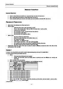
Example Primal system
P)
Dual system
D)
x3
x1 + 3x2 – 2x3 = 6 x1, x2 , x3 > 0 y < 0, y > 0, 3y > 0 6y < 0
intersection = {0}
P (0, 2, 0)
x2
(0, 0, –3)
(6, 0, 0)
xy1 D is clearly incompatible
Comment • The theorems of the alternative provide us with an important mean to tackle the problem of deciding whether a polyhedron is empty or not • They allow us to transform a problem with a universal quantifier (∀) in one with an existence quantifier (∃). In fact a polyhedron Ax < b is empty if for all x ∈ IRn there exists a row i such that aix > bi. The theorems of the alternative make it unnecessary to check that for all x by looking for just one y such that yb < 0 which belongs to another polyhedron (the dual of Ax < b). • As a matter of fact, the difference between an “easy” and a “difficult” problem is often marked by the possibility or impossibility of such a practice. For instance, the very definition of the class NP is based on this distinction.
Duality Theory in LP • Consider an LP problem in standard form: P)
min
cx Ax = b x>0
Theorem (strong duality): A feasible solution x* of problem P is optimal if and only if thare exists a y* belonging to D = {y ∈ IRm: yA < c} such that y*b > cx*
Example Problem
P)
min
i.e.,
D = {y∈IR: D = {y∈IR:
x1 – 2x2 + 4x3 x1 + 3x2 – 2x3 = 6 x1, x2 , x3 > 0 y < 1, 3y < –2 , –2y < 4} y < 1, y < –2/3 , y > –2}
x3 P xy1 x* = (6, 0, 0)
x* non optimal
cx* = +6 >
x2
y* = –2/3
y*b = –4
Example Problem
P)
min
i.e.,
D = {y∈IR: D = {y∈IR:
x1 – 2x2 + 4x3 x1 + 3x2 – 2x3 = 6 x1, x2 , x3 > 0 y < 1, 3y < –2 , –2y < 4} y < 1, y < –2/3 , y > –2}
x3 P xy1
x* optimal
cx* = –4
y* = –2/3
y*b = –4
cx* for some y* ∈ D. Then the system yA < c –yb < –cx* namely y[A, –b] < [c, –cx*] turns out to be compatible. If we apply Gale’s Theorem to such a system we see that the system x x x [A, –b][ ] = 0, [ ] > 0, [c, –cx*][ ] < 0 λ λ λ is necessarily incompatible.
Strong duality Proof (contd.): In other words no x, λ > 0 fulfils Ax = λb, cx < λcx* and this is true, in particular, for λ = 1, which implies that no feasible x for P exists which fulfils cx < cx* and so x* is optimal for P.
Strong duality Proof (contd.): Conversely, if the dual system y[A, –b] < [c, –cx*] is incompatible, then the primal Ax = λb, cx < λcx* has a solution x°, λ° > 0. – If λ° > 0, x°/ λ° is P-feasible and better than x*. – If λ° = 0, one hasAx° = 0, x° > 0 and cx° < 0, hence x* + x° is feasible and better than x*. Therefore, x* is not optimal.
End proof
The dual problem • The theorem just proved justifies the introduction of a new problem D) max yb yA < c • This is called the dual of problem P. In turn, P is called the primal problem. • The dual of a linear program (in standard form) is still a linear program (in general form). • The dual problem has – a variable for each constraint of the primal, – a constraint for each variable of the primal.
Proprieties of the dual Theorem (reciprocity): Problem P is the dual of problem D. Theorem (weak duality or dominance): For any pair x ∈ P, y ∈ D of solutions one has yb < cx. Proof: Reciprocity is readily seen by rewriting D in standard form adding nonnegative slack variables, and then writing the dual of the problem so obtained. To see dominance it suffices to combine the columns of yA < c (constraints of D) using the components of x as multipliers. Since the combination is conic, the inequality is preserved: yAx < cx The thesis is obtained by the associative property (y(Ax) < cx) and by observing that Ax = b.
A few corollaries Corollary: x* ∈ P and y* ∈ D are optimal if and only if y*b = cx* Proof: by combining weak and strong duality. Corollary (complementary slackness): x* ∈ P and y* ∈ D are optimal if and only if (c – y*A)·x* = y*·(Ax* – b) = 0 Proof: this corollary says that optimal dual (primal) slacks are orthogonal to any optimal primal (duale) solution. The first condition rewrites cx* = y*Ax*, and since Ax* = b it is equivalent to the previous corollary. The second one is true ∀y*, because Ax* = b.
Example Primal problem
P)
Dual problem
D)
x3 primal optimum 6
min
4x1 + 3x2 + x3 x1 + 3x2 – 2x3 = 6 x1, x2 , x3 > 0 max 6y y < 4, 3y < 3, –2y < 1
P x1
(0, 2, 0)
dual optimum 6
0
x2
−1/2
1
4
y
A few corollaries Corollary: if problem P (problem D) is unbounded from below (from above) then problem D (problem P) has no solution. Proof: it directly derives from weak duality. For example, suppose by contradiction that P is unbounded from below (i.e., for any x ∈ P there exists an x° ∈ P such that cx° < cx) and that, however, D is non-empty (i.e., there exists one y° ∈ D). This clearly contradicts weak duality, according to which one has y°b < cx, ∀x ∈ P, and therefore it can’t be cx → –∞. (A similar argument can be used for the case D unbounded).
Example Primal problem
P)
Dual problem
D)
x3
min – 4x1 – 3x2 – x3 x1 + 3x2 – 2x3 = 6 x1, x2 , x3 > 0 max 6y y < –4, 3y < –3, –2y < –1
unbounded primal
P x1 0
x2
–4
–1
1/2
empty dual
y
Summarizing P unbounded
P=Ø
P has a finite optimum
D unbounded
impossible
×
impossible
D=Ø
×
?
D has a finite optimum
impossible
impossible
impossible
×
Rules to construct the dual Rule 1:
Rule 2:
Rule 3:
Rule 4:
Write the primal as a minimization problem with > and/or = constraints. The dual will then be a maximization problem with = and/or < constraints. Add a dual variable yi for any primal constraint: yi will be • > 0 if the primal constraint is > (loose constraint) • free if the primal constraints is = (strict constraint) The dual objective function is a linear combination of the yi’s with the primal left-hand side b. The dual hand side is instead the primal cost vector c. Add a dual constraint for any primal variable xj: this constraint will have the form • of < (loose constraint) if xj is > 0 • of = (strict constraint) if xj is free
Example 1 Primal problem
P)
max
Rewrite (Rule 1)
P)
min
Dual problem
D)
max
5x1 – x2 + 2x3 x1 + 4x2 – 6x3 < 6 2x1 – x3 = 4 2x1 + 3x2 > 5 x2, x3 > 0 – 5x1 + x2 – 2x3 – x1 – 4x2 + 6x3 > –6 2x1 – x3 = 4 > 5 2x1 + 3x2 x2, x3 > 0 – 6y1 + 4y2 + 5y3 y1, y3 > 0 – y1 + 2y2 + 2y3 = –5 – 4y1 + 3y3 < 1 6y1 – y2 < –2
Example 2 Primal problem
P)
min
4x1 + 3x2 + x3 x1 + 3x2 – 2x3 = 6 x1, x2 , x3 > 0
x3 primal optimum 39/5 = 7,8
x1 + x2 + x3 > 3
P (6, 0, 0)
(0, 12/5, 3/5) (3/2, 3/2, 0)
x2
x1
What is the dual problem?
Example 3 Primal problem
P)
max min
x3
4x1 + 3x2 + x3 x1 + 3x2 – 2x3 = 6 x1, x2 , x3 > 0 x1 + x2 + x3 > 3
P (6, 0, 0)
(0, 12/5, 3/5) (3/2, 3/2, 0)
x2
x1
What is the dual optimum value? What is the dual problem?