Microstructure Models with Short-Term Inertia and Stochastic Volatility

Hindawi Publishing Corporation Mathematical Problems in Engineering Volume 2015, Article ID 323475, 17 pages http://dx.doi.org/10.1155/2015/323475

Research Article Microstructure Models with Short-Term Inertia and Stochastic Volatility Michael A. Kouritzin Department of Mathematical and Statistical Sciences, University of Alberta, Edmonton, AB, Canada T6G 2G1 Correspondence should be addressed to Michael A. Kouritzin; [email protected] Received 2 March 2015; Revised 9 July 2015; Accepted 15 July 2015 Academic Editor: Quanxin Zhu Copyright © 2015 Michael A. Kouritzin. This is an open access article distributed under the Creative Commons Attribution License, which permits unrestricted use, distribution, and reproduction in any medium, provided the original work is properly cited. Partially observed microstructure models, containing stochastic volatility, dynamic trading noise, and short-term inertia, are introduced to address the following questions: (1) Do the observed prices exhibit statistically significant inertia? (2) Is stochastic volatility (SV) still evident in the presence of dynamical trading noise? (3) If stochastic volatility and trading noise are present, which SV model matches the observed price data best? Bayes factor methods are used to answer these questions with real data and this allows us to consider volatility models with very different structures. Nonlinear filtering techniques are utilized to compute the Bayes factor on tick-by-tick data and to estimate the unknown parameters. It is shown that our price data sets all exhibit strong evidence of both inertia and Heston-type stochastic volatility.

1. Introduction Financial analysts list speculation, finiteness of assets, interest rates, tick size, price inertia, price clustering, belief heterogeneity, asymmetric information, greed and fear, and so forth as causes for price fluctuations over time. Yet, popular models like geometric Brownian motion (GBM) (e.g., Black and Scholes [1], Merton [2]) or the Cox-Ross-Rubinstein model [3] try to handle all these factors in an overly simple framework, resulting in unnatural phenomena like the volatility smile. Consequently, stochastic volatility, which has been observed in real prices, is often added to the price value evolution (e.g., Heston [4], Jachwerth and Rubinstein [5], Hull and White [6], and Nelson [7]) to avoid the volatility smile. However, which stochastic volatility model fits the market data best? Nowadays, many authors talk about the misspecification of stochastic price-volatility models (including the Heston model which we show favorably herein) so much. It leads us to wonder whether there are missing ingredients to these very simple models. Even combined stochastic value-volatility models do not address tick size, price inertia, price clustering, hidden liquidity, and fear-greed cycles that traders, especially high frequency traders, must deal with. To handle these

issues, one is drawn to tick-by-tick microstructure models and left with the perplex question: How should one model price inertia in continuous time? We are using the term price inertia instead of the related term price momentum because we are not weighting transaction prices by volume. Fractional Brownian motion (FBM), best known for its long memory properties, exhibits inertia and has been used to model markets (Mandelbrot [8], Shiryaev [9]) even though these models allow arbitrage strategies. We speculate that FBM’s success in modeling observed data is more attributable to inertia than long memory. However, we introduce an alternative inertia process and show that this new process better satisfies the desired properties of inertia than FBM. We then show strong statistical evidence of price inertia that lasts for hours or days using Bayes estimates and Bayes factor on real price data. We do not consider the possibility of arbitrage nor determine derivative prices for our models but rather leave these interesting mathematical finance questions to the experts. (See Capinski and Zastawniak [10] for an excellent introduction to these types of questions and to mathematical finance in general.) Also, we leave the difficult task of obtaining theoretical error bounds for our particle filter methods to other works. (See, e.g., Kouritzin and Zeng [11] and Del Moral et al. [12] for related work on approximate

2 filters.) Our focus is solely on modeling observed stock price data and the methodology of determining which of a class of models best fits the observed data. High frequency data contains complete marketparticipant trading activities (Engle [13]) and is modeled using microstructure (Black [14], Chan and Lakonishok [15], Hasbrouck [16, 17], Engle and Russell [18], Engle [13], and Bandi and Russell [19]). Unlike the macrostructure market, the trading noise in the microstructure market is not negligible; thus, the intrinsic asset value is not readily discernable. In this paper, we introduce a class of dynamic microstructure models, where the transaction price is formulated as a distorted and color-noise corrupted variant of the intrinsic asset value with the intrinsic asset value being a traditional stochastic value-volatility process. Indeed, we view the transaction price data as random counting-measure observations of intrinsic value corrupted by microstructure trading noise with such things as inertia and fear-greed cycles built in. However, trading noise sources themselves introduce volatility to transaction prices. This raises the question, “Do we need to model stochastic volatility explicitly in the presence of dynamic microstructure trading noise?” We will give strong evidence of the presence of stochastic volatility through Bayes factor methods and stochastic filtering theory. Moreover, we also utilize model selection to provide strong evidence of Heston-type volatility over competing stochastic volatility models based on the observed transaction data in a microstructure market. This suggests that the common viewpoint of the Heston model being highly misspecified might be better stated as overly simplistic macrostructureonly models are underspecified. Bayes factor (see, e.g., Kass and Raftery [20]) is our preferred model selection method since it provides statistical comparisons in real time as to which model best fits the market data while allowing the stochastic value-volatility (signal) models to be singular to one another. Indeed, to use the Bayes factor method, we need only to be able to transform all microstructure asset-price observation models of interest into the same canonical process via Girsanov-type measure change. Previously, Zeng [21] studied a filtering equation for inferring the intrinsic value process in a microstructure model while Xiong and Zeng [22] proposed a branching particle approximation to this equation. Kouritzin and Zeng [23] derived a Bayes factor equation and discussed the Bayesian model selection problem to determine whether financial data, such as stock prices, display jump-type stochastic volatility. However, all these works are based on a restricted microstructure model and thus cannot be applied to our general setting. Moreover, our problems of showing statistical evidence of inertia and determining which of the classical stochastic volatility models best represents real data in the presence of microstructure noise were not considered. We also propose a new inertia process, explain its role in modeling prices, and show its statistical significance with real tick-by-tick data. Section 2 is devoted to explaining our model. First, our five standard value-volatility models (GBM, Hull-White, Log Ornstein-Uhlenbeck, continuous GARCH, and Simplified Heston) are given followed by our microstructure inertia process and its properties and then the other components

Mathematical Problems in Engineering of our dynamic microstructure model. Together the valuevolatility and microstructure components form our price evolution model, which, at the end of Section 2, is interpreted as a filtering model. In Section 3, we discuss model calibration and fair price/value estimation through Bayesian filter estimation. A filtering equation and a branching particle filter approximation algorithm are first given and explained. Then, their use to identify parameters and come up with initial state estimates is discussed. Finally, numeric parameter and initial state estimates for each model are given. As a byproduct, it is demonstrated that proper modeling and estimation of fair price (as is done herein) can provide information about overbought conditions and help avoid financial loss (see Figure 4). Section 4 is dedicated to Bayesian model selection. We first motivate the use of Bayes factor for model selection and explain how to estimate Bayes factor from unnormalized particle filters. Then, we establish strong statistical evidence of inertia and Heston-type volatility in all our price data through model selection using the Bayes factor method to test which fair price-volatility model and what amount of inertia best fit the observed price data.

2. The Partially Observed Market Model In this section, we build our stochastic model that has macrostructure and microstructure components and interpret this model in terms of a signal that needs to be estimated in real time and observations which are used to form the signal estimates. The macrostructure model consists of fair price, volatility, and related parameters and will be denoted by (𝑋, 𝜃) in the sequel, with 𝑋 = (𝑆, 𝑉) being price and volatility and 𝜃 being the parameters for this model. Unlike macrostructure models, we do not assume access to (𝑋, 𝜃), but rather we take it to be part of the signal to be estimated. Indeed, a model would be judged to be better if the macrostructure price 𝑆 (which represents a “fair” price) is quite different than the observed price and we can use filtering to determine overbought and oversold situations. The microstructure price construction converts the macrostructure model into the observed price. Such things as inertia (or momentum), fear-greed cycles, and wholeprice clustering (or rounding), which are not part of the fair price, are incorporated into the microstructure model. A distinguishing feature in our microstructure is dynamic state: To allow the microstructure to influence price over a period of time so that the observed microstructure price can differ from fair price significantly, one needs to add and then estimate microstructure state 𝑍. In particular, the inertia process, characterized by a parameter ℎ, is introduced to capture price inertia that might be caused by hidden liquidity; various reaction and access times to information as well as momentum traders themselves. This inertia process is not ̂ℎ Markov, so we will have to consider the historical version 𝑍 ℎ ̂ is also unobservable and hence must of this state. Further, 𝑍 be added to the signal along with microstructure parameters 𝜗 and all must be estimated as nuisance parameters. The nondynamic part of the microstructure noise consists of rounding and clustering noise. It is widely observed in

Mathematical Problems in Engineering

3

markets that more trades occur at more even prices like whole nickel or whole dollar levels. Therefore, to match observed prices well, we should have a mechanism to convert evenly distributed raw prices into whole-price-biased observed prices. This is done by binning raw prices into sets 𝐷1 , 𝐷2 , 𝐷3 , 𝐷4 , and 𝐷5 depending on how even they are and then randomly moving raw prices in the less even bins to close prices in the more even bins in order to match the observed prices. The observations then become the marked counting process of the number of trades that occur at the various prices. We will later use these observations to select and calibrate models and to estimate the augmented signal: ̂ℎ ) . (𝑋, 𝜃, 𝜗, 𝑍

Example 3 (GBM model; see Black and Scholes [1], Merton [2]). We have that 𝑑𝑆𝑡 = 𝜇𝑑𝑡 + 𝜎𝑑𝑊𝑡 , 𝑆𝑡

(1)

The whole point of the microstructure is to allow the macrostructure price to distinguish itself from the observations and rather to represent fair value. We then use filtering on asset prices to estimate implied value (hereafter called fair price) and thereby judge whether an asset is overbought or oversold. 2.1. General Notation. Let [0, 𝑇] be a fixed time period and let (Ω, F, (F𝑡 )0≤𝑡≤𝑇 , P) be a complete filtered probability space. For any stochastic process 𝜌, its natural filtration, defined as 𝜌 F𝑡 ≐ 𝜎{𝜌𝑢 : 0 ≤ 𝑢 ≤ 𝑡}, represents the information in 𝜌 up to time 𝑡. N0 denotes the set of nonnegative integers and, for any Polish space 𝐸, 𝐵(𝐸) is the set of all bounded measurable R-valued functions on 𝐸. 2.2. Common Macrostructure State Models. We use a macrostructure model 𝑀 = (𝑋, 𝜃) for the unobservable fair price together with its volatility and parameters. Here, 𝑋 ∈ R𝑛𝑥 is the macrostructure financial state (fair price plus volatility) with macrostructure parameter 𝜃 ∈ R𝑛𝜃 for some 𝑛𝑥 , 𝑛𝜃 ∈ N0 . We let 𝜇 be a probability distribution on R𝑛𝑥 +𝑛𝜃 , take A to be a generator with domain D(A) ⊂ 𝐵(R𝑛𝑥 +𝑛𝜃 ), and assume (𝑋, 𝜃) satisfies the martingale problem. Definition 1. (𝑋, 𝜃) is the unique solution of the R𝑛𝑥 +𝑛𝜃 valued martingale problem for A with initial distribution 𝜇. That is,

(3)

with parameters 𝜃 = (𝜇, 𝜎), corresponds to our martingale problem with the generator 𝑑𝑓 𝑑2 𝑓 1 A(1) 𝑓 = 𝜎2 𝑠2 2 + 𝜇𝑠 . 2 𝑑𝑠 𝑑𝑠

(4)

In GBM model, the volatility 𝜎 is a constant. To account for the “volatility smile” commonly observed in market option prices (see Jackwerth and Rubinstein [5] for a detailed survey), the GBM model is generalized to stochastic volatility (SV) models, where 𝜎 itself is replaced by a stochastic process {𝑉𝑡1/2 , 𝑡 ≥ 0}. Some of the popular SV models include the following. Example 4 (Hull-White model; see Hull and White [6]). Consider 𝑑𝑆𝑡 = 𝜇𝑑𝑡 + 𝑉𝑡1/2 𝑑𝑊𝑡 , 𝑆𝑡 𝑑𝑉𝑡 = ]𝑑𝑡 + 𝜅𝑑𝐵𝑡 , 𝑉𝑡

(5)

with parameters 𝜃 = (𝜇, ], 𝜅) and generator 𝜕𝑓 1 𝜕𝑓 𝜕2 𝑓 1 𝜕2 𝑓 A(2) 𝑓 = V𝑠2 2 + 𝜇𝑠 + 𝜅2 V2 2 + ]V . 2 𝜕𝑠 𝜕𝑠 2 𝜕V 𝜕V

(6)

Example 5 (Logarithmic Ornstein-Uhlenbeck model; see Scott [26]). We have that

−1

(i) 𝜇 = P ∘ (𝑋0 , 𝜃) , 𝑓

general enough to cover most interesting financial models. In this paper, the macrostructure state 𝑋 consists of two components: the fair price 𝑆 and the stochastic volatility 𝑉 (if any). The most common example of (𝑆, 𝑉, 𝜃) in finance is the “geometric Brownian motion” (GBM) utilized in the classical Black-Scholes option pricing formula. Throughout this section, 𝑊 and 𝐵 are two independent standard Brownian motions and (𝑠, V, 𝜃) ∈ R𝑛𝑥 +𝑛𝜃 .

𝑡

(ii) 𝑀𝑡 = 𝑓 (𝑋𝑡 , 𝜃) − 𝑓 (𝑋0 , 𝜃) − ∫ A𝑓 (𝑋𝑠 , 𝜃) 𝑑𝑠

(2)

0

̃ ̃ is {F𝑋,𝜃 𝑡 }-martingale for each 𝑓 ∈ D(A). Moreover, if (𝑋, 𝜃) ̃ ̃ also satisfies (i) and (ii), then (𝑋, 𝜃) and (𝑋, 𝜃) have the same finite dimensional distributions. Remark 2. While 𝜃 does not vary in time, we include it in our macrostructure model to be estimated because it is still unknown. Nevertheless, the operator A does not act on the variable 𝜃 since 𝑑𝜃𝑡 /𝑑𝑡 = 0 for our fixed parameters. The martingale problem formulation (2) (see Stroock and Varadhan [24], Ethier and Kurtz [25] for more details) is

𝑑𝑆𝑡 = 𝜇𝑑𝑡 + 𝑉𝑡1/2 𝑑𝑊𝑡 , 𝑆𝑡 𝑑𝑉𝑡1/2 𝑉𝑡1/2

1 = ( ]2 − 󰜚 (ln 𝑉𝑡1/2 − 𝜛)) 𝑑𝑡 + 𝜅𝑑𝐵𝑡 , 2

(7)

with parameters 𝜃 = (𝜇, ], 󰜚, 𝜛, 𝜅) and generator 𝜕𝑓 1 𝜕2 𝑓 𝜕2 𝑓 1 A(3) 𝑓 = V2 𝑠2 2 + 𝜇𝑠 + 𝜅2 V2 2 2 𝜕𝑠 𝜕𝑠 2 𝜕V 𝜕𝑓 1 + V ( ]2 − 󰜚 (ln V − 𝜛)) . 2 𝜕V

(8)

4


Example 6 (continuous GARCH model; see Nelson [7]). We have that 𝑑𝑆𝑡 = 𝜇𝑑𝑡 + 𝑉𝑡1/2 𝑑𝑊𝑡 , 𝑆𝑡

(9)

𝑑𝑉𝑡 = (] − 󰜚𝑉𝑡 ) 𝑑𝑡 + 𝜅𝑉𝑡 𝑑𝐵𝑡 , with parameters 𝜃 = (𝜇, ], 󰜚, 𝜅) and generator 𝜕𝑓 1 𝜕2 𝑓 1 𝜕2 𝑓 A(4) 𝑓 = V𝑠2 2 + 𝜇𝑠 + 𝜅2 V2 2 2 𝜕𝑠 𝜕𝑠 2 𝜕V 𝜕𝑓 + (] − 󰜚V) . 𝜕V

(10)

Example 7 (simplified Heston model; see Heston [4]). We have that 𝑑𝑆𝑡 = 𝜇𝑑𝑡 + 𝑉𝑡1/2 𝑑𝑊𝑡 , 𝑆𝑡 𝑑𝑉𝑡 = (] − 󰜚𝑉𝑡 ) 𝑑𝑡 +

(11)

𝜅𝑉𝑡1/2 𝑑𝐵𝑡 ,

with parameters 𝜃 = (𝜇, ], 󰜚, 𝜅) and generator 𝜕𝑓 1 𝜕2 𝑓 𝜕𝑓 1 𝜕2 𝑓 A(5) 𝑓 = V𝑠2 2 + 𝜇𝑠 + 𝜅2 V 2 + (] − 󰜚V) . (12) 2 𝜕𝑠 𝜕𝑠 2 𝜕V 𝜕V

We label this example as simplified because we do not allow 𝐵 and 𝑊 to be correlated as Heston did. There is no mathematical issue by including this correlation, but it would add a parameter to the model, which increases computation time. The Heston model already performed the best without this parameter. GBM (with microstructure) plays a special role in our study as it is our no stochastic volatility model. We will compare our other models against it on real data to determine whether stochastic volatility is present. In summary, refer to Table 1. Remark 8. The continuous GARCH model is the continuoustime limit of many classical GARCH-type discrete-time processes (Nelson [7], Drost and Werker [27]). We did not consider jumping stochastic volatility models (e.g., Elliott et al. [28], Kouritzin and Zeng [23], Duffie et al. [29], Eraker et al. [30], and Eraker [31]) or models where 𝑊, 𝐵 are correlated, due to our need to dedicate our limited computer resources to handling our complicated (non-Markov) microstructure with inertia. Still, we want to emphasize that the computational complexity we experienced is fundamental to the fact that we are using non-Markov (inertia) models and has little to do with our particular methods. Indeed, our Bayes factor filtering methods are what makes the computations possible on an inexpensive contemporary desktop computer. 2.3. Construction of Microstructure Price. The fair pricevolatility models account for the random variances of the intrinsic asset value; thus, the selection of proper SV model is crucial for investing, derivative pricing, and hedging. On the other hand, microstructure noise (see Black [14], Hansen and Lunde [32], Duan and Fulop [33], etc.) causes random

Table 1 Name Model GBM 𝑀(1) Hull-White 𝑀(2) Log O-U 𝑀(3) GARCH 𝑀(4) Heston 𝑀(5)

Macrostate 𝑆 (𝑆, 𝑉) (𝑆, 𝑉) (𝑆, 𝑉) (𝑆, 𝑉)

Macroparameter (𝜇, 𝜎) (𝜇, ], 𝜅) (𝜇, ], 󰜚, 𝜛, 𝜅) (𝜇, ], 󰜚, 𝜅) (𝜇, ], 󰜚, 𝜅)

Generator A(1) A(2) A(3) A(4) A(5)

perturbations of transaction price from its intrinsic value and the disregard of such trading noise introduces severe bias into stochastic volatility estimation (see Duan and Fulop [33]). We incorporate microstructure trading noise into traditional fair price-volatility models and use statistical filtering to reveal such things as short-term inertia in the trading noise and stochastic volatility in the intrinsic value. In microstructure markets, the price changes occur only at irregularly spaced transaction times 𝑡1 , 𝑡2 , . . . with total trading intensity 𝑎(𝑡) (see Engle [13]). Here, we assume 𝑎(𝑡) is just a time-varying measurable function as the empirical analysis illustrates that there is no need to consider more general structures. At each transaction time 𝑡𝑖 , the transaction price 𝑌𝑡𝑖 is formulated as 𝑌𝑡𝑖 = 𝐹 (𝑋𝑡𝑖 , 𝑡𝑖 ) ,

(13)

where 𝐹 is some nonlinear random field modeling the trading noise. Formulation (13) is similar to that of Hasbrouck [16], where 𝑋 is the intrinsic and permanent component while 𝐹 introduces the transitory component. The empirical evidence reported by Hansen and Lunde [32] suggests strongly that the trading noise is serially correlated. Similar results can be found in A¨ıt-Sahalia et al. [34]. Indeed, there exist situations in which the trading noise variance estimate is zero if the trading noise is simply assumed to be independent (see Duan and Fulop [33]). This does not mean there is no trading noise but rather that the trading noise is autocorrelated. To characterize this correlation, Hansen and Lunde [32] assume the trading noise to be some Gaussian random sequence with stationary covariance and finite dependence. However, this model is most suitable for the low-frequency data and ignores many crucial microstructure effects. We build correlation into our microstructure information noise through inertia and mean-reversion while utilizing microstructure rounding and clustering noise to explain the discreteness and whole-price biasing. 2.3.1. Inertia. The idea of momentum or inertia has been used in many studies (see Jegadeesh and Titman [35], Moskowitz and Grinblatt [36], Grundy and Martin [37], Grundy et al. [38], etc.). Basically, there is the tendency for a stock to continue to move in one direction. To illustrate our approach, we introduce the following definition.


5

Definition 9. A process (𝑍𝑡 ) is said to have stochastic inertia at time 𝑡 if 𝐼𝑡𝑍

𝜕 𝜕 ≐ lim E [𝑍𝑢 𝑍𝑡 ] ∈ (0, ∞] . 𝑢↘𝑡 𝜕𝑡 𝜕𝑢

Definition 10. Our stochastic inertia process is 𝑡

𝜉𝑡ℎ = √ℎ ∫ tanh (

(14)

0

(𝑡 − 𝑠) ) 𝑑𝐵𝑠𝜉 + √1 − ℎ𝑊𝑡𝜉 , Δ

(18)

𝐼𝑡𝑍 is called the inertia function.

where (𝐵𝜉 , 𝑊𝜉 ) is a 2-dimensional standard Brownian motion, Δ > 0, and 0 ≤ ℎ ≤ 1.

The idea behind our definition is that for inertia we should expect 𝑍𝑢+𝑟 −𝑍𝑢 and 𝑍𝑡 −𝑍𝑡−𝑘 to have the same sign for 𝑢 > 𝑡, but close to 𝑡 and 𝑟, 𝑘 > 0 small. We strengthen this condition to

Remark 11. 𝜉𝑡ℎ is a weighted average of the historical information (the first term) and fundamental information (the second term). In fact, tanh(𝑡/Δ) can be viewed as the impulse response on price created by market participants receiving and simulating the “information” 𝑑𝐵𝑡𝜉 and Δ determines the diffusion speed in the market. This formulation captures the idea that news or rumor and its ramifications require time to be fully disseminated and understood. When ℎ = 1, it represents the case of only historical information resulting in the strongest inertia in prices. Alternatively, we can use inertia to explain “hidden liquidity.” If everybody knew that an agent was going to make a big change in a position, then the price would immediately jump. However, if the agent breaks up the desired change into small transactions, then it takes time for this extra buying or selling pressure to be recognized in the market. In this case, ℎ = 1 represents the case, where all changes in position are done over a period of time and Δ represents the time to effect 58% of the positional change.

lim lim lim

𝑢↘𝑡 𝑘 → 0 𝑟 → 0

𝐸 [(𝑍𝑢+𝑟 − 𝑍𝑢 ) (𝑍𝑡 − 𝑍𝑡−𝑘 )] >0 𝑟𝑘

⇐⇒ lim lim [ lim 𝑢↘𝑡 𝑘 → 0

𝑟→0

𝐸 [(𝑍𝑢+𝑟 − 𝑍𝑢 ) 𝑍𝑡 ] 𝑟𝑘

𝐸 [(𝑍𝑢+𝑟 − 𝑍𝑢 ) 𝑍𝑡−𝑘 ] − lim ]>0 𝑟→0 𝑟𝑘 ⇐⇒ lim 𝑢↘𝑡

(15)

𝜕 𝜕 𝐸 [𝑍𝑢 𝑍𝑡 ] > 0. 𝜕𝑡 𝜕𝑢

Many processes have inertia. However, to model the stock price effect of the information reaching all market participants, we want the following five properties: (1) 𝑍𝑡 is Gaussian and driftless and Var(𝑍𝑡 ) is proportional to 𝑡 so 𝑍 resembles Brownian motion; (2) 𝐼𝑡𝑍 is finite, not infinite, indicating that the influence of past values on immediate future is not too strong; (3) 𝑍𝑡 makes sense from informational and hidden liquidity points of view; more precisely, it can explain well the price effects due to the reactions of all market participants to information and rumor being diffused and simulated over a period of time as well as due to the purchases or sales of an agent spreading out a large change in his/her position over time; (4) 𝑍 is easy to simulate using, for example, the Gaussian property; (5) 𝑍 is easy to analyze. Neither a Brownian motion 𝐵 nor more generally a square integrable martingale has inertia. Brownian motion with drift 𝑡 𝑍𝑡 = 𝑍0 + ∫0 𝑚(𝑍𝑠 )𝑑𝑠 + 𝐵𝑡 has inertia 𝐼𝑡𝑍 = 𝐸[𝑚2 (𝑍𝑡 )] but we do not want drift. For fractional Brownian motion (FBM) 𝐵ℎ , E [𝐵𝑡ℎ 𝐵𝑢ℎ ] =

1 (|𝑡|2ℎ + |𝑢|2ℎ − |𝑢 − 𝑡|2ℎ ) , 2

(16)

where ℎ ∈ (0, 1) is the Hurst parameter. Therefore, 𝜕 𝜕 E [𝐵𝑡ℎ 𝐵𝑢ℎ ] = lim ((2ℎ − 1) ℎ (𝑢 − 𝑡)2ℎ−2 ) = ∞ 𝑢↘𝑡 𝜕𝑡 𝜕𝑢 𝑢↘𝑡

𝑡

E [𝜉𝑡ℎ 𝜉𝑢ℎ ] = ℎ ∫ tanh ( 0

(𝑡 − 𝑠) (𝑢 − 𝑠) ) tanh ( ) 𝑑𝑠 Δ Δ

is positive for any 𝑢 ≥ 𝑡. In particular, Var (𝜉𝑡ℎ ) 𝑡

=

ℎ 𝑡 (𝑡 − 𝑠) ) 𝑑𝑠 + (1 − ℎ) ∫ tanh2 ( 𝑡 0 Δ

tanh (𝑡/Δ) . = 1 − ℎΔ 𝑡

(20)

Thus, Var(𝜉𝑡ℎ )/𝑡 converges to 1 as 𝑡 → ∞ with speed determined by Δ. (Hence, informational noise increases at the same asymptotic rate as Brownian motion.) Moreover,

(17)

Thus, the inertia function of 𝐵ℎ is infinity for all 𝑡 if ℎ > 1/2 (and is −∞ if ℎ < 1/2). Neither case satisfies our five properties. Still, standard representations of FBM motivate the creation of driftless inertia by convolving a Brownian motion with the desired impulse response for information dissemination. With this in mind, we consider the following inertia process.

(19)

+ (1 − ℎ) 𝑡

𝜕 𝜕 E [𝜉𝑡ℎ 𝜉𝑢ℎ ] 𝜕𝑡 𝜕𝑢

lim

1 if ℎ > . 2

Note that 𝜉𝑡ℎ is a centered Gaussian process such that the autocovariance

ℎ 𝑡 (𝑡 − 𝑠) (𝑢 − 𝑠) = 2 ∫ sech2 ( ) sech2 ( ) 𝑑𝑠 Δ 0 Δ Δ

(21)

and, using standard antiderivatives, 𝜕 𝜕 ℎ 𝑡 𝑠 E [𝜉𝑡ℎ 𝜉𝑢ℎ ] = 2 ∫ sech4 ( ) 𝑑𝑠 𝑢↘𝑡 𝜕𝑡 𝜕𝑢 Δ 0 Δ

lim

ℎ 𝑡 tanh3 (𝑡/Δ) = [tanh ( ) − ]. Δ Δ 3

(22)

6

Mathematical Problems in Engineering ℎ

Thus, the inertia function of our inertia process is 𝐼𝑡𝜉 = (ℎ/Δ)[tanh(𝑡/Δ) − tanh3 (𝑡/Δ)/3], the steady-state inertia is

2.00

ℎ tanh3 (𝑡/Δ) 2ℎ 𝑡 , ]= [tanh ( ) − 𝑡→∞Δ Δ 3 3Δ

1.60

(23)

and this happens quickly for small Δ. We can thus verify that 𝜉ℎ , defined in (18), satisfies our five desired properties. One can also look upon Δ as the time for new information to be disseminated to fifty-eight percent of the market. Below, we consider three different dissemination times: Δ = 40 minutes, Δ = 2 hours, and Δ = 1/2 day on real stock data. Finally, the fact that 𝜉ℎ is Gaussian eases its simulation greatly. 2.3.2. Information Noise and Augmented State. Hitherto, we have focused on constructing inertia processes. Now, we include all informational noise into asset prices. Information noise is introduced to represent trading noises due to things like inertia, fear-greed cycles, belief heterogeneity, and asymmetric information. For the 𝑖th-transaction occurring at 𝑡𝑖 , the raw price Y𝑡𝑖 is defined by ln Y𝑡𝑖 ℎ,Δ {ln 𝑆𝑡𝑖 + 𝑍𝑡𝑖 + 𝜖𝜁𝑖 , dynamical microstructure, (24) ={ ln 𝑆 + 𝜖𝜁𝑖 , nondynamical, { 𝑡𝑖

𝑑𝑍𝑡ℎ,Δ = −𝜙𝑍𝑡ℎ 𝑑𝑡 + 𝑑𝜉𝑡ℎ ,

𝑍0ℎ,Δ = 𝑧0 ,

(25)

where 𝑍ℎ,Δ is the dynamical part of the microstructure through which inertia is introduced (with our inertia process 𝜉ℎ ) and 𝑋 = (𝑆, 𝑉). The case 𝑍ℎ,Δ ≡ 0 is of particular importance in the sequel as it represents the nondynamical microstructure case and is used as a calibration model. The information noise consists of two parts: 𝜁 = {𝜁𝑖 }∞ 𝑖=1 is a sequence of independent standard Gaussian random variables, 𝜖 > 0; 𝑍ℎ is Ornstein-Uhlenbeck- (O-U-) like inertia velocity process with mean-reverting parameter 𝜙 > 0. Here, 𝜉ℎ , 𝜁, and 𝑋 are independent and 𝑧0 is a constant. 𝑍ℎ provides an intuitive continuous-time model that accommodates the joint presence of the inertia and mean-reversion. Our information noise is more reasonable than that of Zeng [21] in that (1) we preclude the possibility of negative prices by using multiplicative noise; (2) the stochastic inertia process 𝜉ℎ captures the empirical feature of the inertia observed in transaction prices (e.g., Jegadeesh and Titman [35]); (3) the mean-reverting structure of 𝑍ℎ when combined with the inertia captures the cyclic property of prices (e.g., Black [14]). 𝑍ℎ is not a Markov process, so we introduce its historical process as ̂ℎ (𝜏) ≐ 𝑍ℎ , 𝑍 𝑡 𝑡∧𝜏

(26)

̂ℎ ∈ 𝐶[0, 𝑇], the space of which is Markovian. Moreover, 𝑍 𝑡 all continuous functions on [0, 𝑇], since the paths of 𝑍ℎ are continuous. Consequently, we augment the state vector to be ̂ℎ ) , (𝑋, 𝜃, 𝜗, 𝑍

(27)

1.40 Trade (%)

lim

1.80

1.20 1.00 0.80 0.60 0.40 0.20 0.00

0 5 10 15 20 25 30 35 40 45 50 55 60 65 70 75 80 85 90 95 Cents

Figure 1: Clustering for 3 stocks in April 2010.

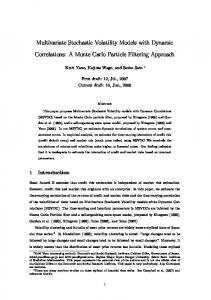
where 𝜗 = (𝜖, 𝜙) is the microstructure noise parameter set. The advantage of this formulation is that we can estimate ̂ℎ and thus 𝑍ℎ jointly with other components using particle 𝑍 filtering methods. The generalized state incorporates fair price, volatility, parameters, and the historical trading noise ̂ℎ while keeping the tractability of a Markovian framework. 𝑍 Remark 12. We include neither ℎ nor Δ into the model parameters but rather consider different models corresponding to different values of ℎ and Δ as well as different SV models 1–5. Indeed, we will provide evidence of inertia in the sequel by using Bayesian methods to select a model with a large value of ℎ based upon tick-by-tick stock data. 2.3.3. Rounding and Clustering Noise. Our final modeling goal is to convert uniform raw price into observed wholeprice-biased price. While raw price Y𝑡𝑖 can take any value, the trading price 𝑌𝑡𝑖 is restricted to multiples of the tick, {𝑦0 = 0, 𝑦1 = 1/𝑀, . . . ,𝑦𝑗 = 𝑗/𝑀, . . .}, for some positive integer 𝑀. The tick size in New York Stock Exchange (NYSE) was switched to $1/16 from $1/8 in June 24, 1997, and then further to $0.01 from January 29, 2001. The empirical studies suggest that the tick size 1/𝑀 plays an important role in microstructure market analysis (e.g., Huang and Stoll [39]). Since we are concerned with price clustering for decimal pricing in stock markets, we let 𝑀 = 100. It is well documented that there is price clustering to more whole prices. To quantify this price clustering, we examine the price behavior for three NYSE-listed stocks over April 2010 (Figure 1 and Table 2). (In a larger study, we considered eight NYSE stocks in different sectors. However, we only report on three here to conserve space. The results for the other five were similar in nature.) The transaction data of these stocks shows there is modest clustering at multiples of 5 cents as shown in Figure 1, plotted in terms of pennies. Supposing the raw price Y𝑡𝑖 falls in the interval [𝑦𝑗 − 1/2𝑀, 𝑦𝑗 + 1/2𝑀), then if there was no clustering noise, the trading price 𝑌𝑡𝑖 would just be 𝑦𝑗 . Thus,


7

Table 2 NYSE stock Goldman Sachs International Business Machines Corporation PepsiCo Inc.

Ticker symbol GS IBM PEP

the probability of trading at 𝑦𝑗 with no clustering noise given 𝑋𝑡𝑖 = 𝑥, 𝑍𝑡𝑖 = 𝑧 would be ln((𝑦𝑗 +1/2𝑀)/(𝑥⋅𝑒𝑧 ))

dynamic microstructure

Case 1. If the fractional part of 𝑦𝑗 belongs to 𝐷1 , 𝑝 (𝑦𝑗 | 𝑥, 𝑧, 𝜗) = 𝑅 (𝑦𝑗 | 𝑥, 𝑧, 𝜗) (1 − 𝛼) . 𝑝 (𝑦𝑗 | 𝑥, 𝑧, 𝜗) = 𝑅∗ (𝑦𝑗 | 𝑥, 𝑧, 𝜗) (1 − 𝛽) ,

(28)

𝑅∗ (𝑦𝑗 | 𝑥, 𝑧, 𝜗) ≐ 𝑅 (𝑦𝑗 | 𝑥, 𝑧, 𝜗) + 𝛼 (𝑅 (𝑦𝑗−1 | 𝑥, 𝑧, 𝜗) + 𝑅 (𝑦𝑗−2 | 𝑥, 𝑧, 𝜗))

̂ℎ , 𝜗) 𝑅 (𝑦𝑗 | 𝑋𝑡𝑖 , Π𝑡𝑖 𝑍 𝑡𝑖 =∫

ln((𝑦𝑗 −1/2𝑀)/𝑋𝑡𝑖 𝑒

̂ℎ Π𝑡 𝑍 𝑖 𝑡𝑖

̂ℎ Π𝑡 𝑍 𝑖 𝑡𝑖

)

)

1 −𝑢2 /2𝜖2 𝑑𝑢, 𝑒 √2𝜋𝜖

Case 3. If the fractional part of 𝑦𝑗 belongs to 𝐷3 , 𝑝 (𝑦𝑗 | 𝑥, 𝑧, 𝜗) = 𝑅∗∗ (𝑦𝑗 | 𝑥, 𝑧, 𝜗) (1 − 𝛾1 − 𝛾2 ) , (30)

Clearly, 𝑅(𝑦𝑗 | 𝑥, 𝑧, 𝜗) is a smooth function of (𝑥, 𝑧, 𝜗) for each fixed 𝑦𝑗 . To build the observed whole-price bias into our model, we introduce the following sets:

(35)

where 𝑅∗∗ (𝑦𝑗 | 𝑥, 𝑧, 𝜗) ≐ 𝑅∗ (𝑦𝑗 | 𝑥, 𝑧, 𝜗) + 𝛽 (𝑅∗ (𝑦𝑗−5 | 𝑥, 𝑧, 𝜗) + 𝑅∗ (𝑦𝑗−10 | 𝑥, 𝑧, 𝜗))

(36)

+ 𝛽 (𝑅∗ (𝑦𝑗+5 | 𝑥, 𝑧, 𝜗) + 𝑅∗ (𝑦𝑗+10 | 𝑥, 𝑧, 𝜗)) .

𝐷1 = {The integers in (0, 100]

Case 4. If the fractional part of 𝑦𝑗 belongs to 𝐷4 ,

that are not multiples of 5} ,

𝑝 (𝑦𝑗 | 𝑥, 𝑧, 𝜗) = 𝑅∗∗ (𝑦𝑗 | 𝑥, 𝑧, 𝜗)

𝐷2 = {The integers in (0, 100] that are multiples of 5 but not of 25} ,

(34)

+ 𝛼 (𝑅 (𝑦𝑗+1 | 𝑥, 𝑧, 𝜗) + 𝑅 (𝑦𝑗+2 | 𝑥, 𝑧, 𝜗)) .

(29)

where Π𝑡𝑖 is the projection onto time 𝑡𝑖 ; that is, ̂ℎ = 𝑍 ̂ℎ (𝑡𝑖 ) = 𝑍ℎ = 𝑍ℎ . Π𝑡𝑖 𝑍 𝑡𝑖 𝑡𝑖 𝑡𝑖 ∧𝑡𝑖 𝑡𝑖

(33)

where

nondynamical.

Equivalently, we can write 𝑅 in terms of the historical process as

ln((𝑦𝑗 +1/2𝑀)/𝑋𝑡𝑖 𝑒

(32)

Case 2. If the fractional part of 𝑦𝑗 belongs to 𝐷2 ,

𝑅 (𝑦𝑗 | 𝑥, 𝑧, 𝜗) ≐ 𝑃 (Y𝑡𝑖 = 𝑦𝑗 | 𝑋𝑡𝑖 = 𝑥, 𝑍𝑡𝑖 = 𝑧, 𝜗) 1 −𝑢2 /2𝜖2 { { 𝑑𝑢 𝑒 ∫ { { ln((𝑦𝑗 −1/2𝑀)/(𝑥⋅𝑒𝑧 )) √2𝜋𝜖 = { ln((𝑦𝑗 +1/2𝑀)/𝑥) { 1 −𝑢2 /2𝜖2 { {∫ 𝑑𝑢 𝑒 √ ln((𝑦 −1/2𝑀)/𝑥) 2𝜋𝜖 𝑗 {

tick level in 𝐷3 ∪ 𝐷4 ∪ 𝐷5 with probability 𝛽. Finally, if the fractional part of the price 𝑦 is in 𝐷3 , then it will stay in the same level with probability 1 − 𝛾1 − 𝛾2 or move to the closest tick level in 𝐷4 with probability 𝛾1 and the closest tick level in 𝐷5 with probability 𝛾2 . In summary, the transition probability function is obtained iteratively by the following.

(31)

𝐷3 = {25, 75} , 𝐷4 = {50} , 𝐷5 = {100} . While the raw price will be uniformly distributed over 𝐷1 ∪ 𝐷2 ∪𝐷3 ∪𝐷4 ∪𝐷5 (or rather the continuous interval (0, 100]), the observed price model must bias 𝐷2 over 𝐷1 , 𝐷3 over either 𝐷2 or 𝐷1 , and so forth. We distribute the observed price randomly over 𝐷1 ∪ 𝐷2 ∪ 𝐷3 ∪ 𝐷4 ∪ 𝐷5 based upon the raw price in a biased manner favoring the more whole-price ticks in 𝐷2 ∪ 𝐷3 ∪ 𝐷4 ∪ 𝐷5 . In particular, if the fractional part of the raw price 𝑦 rounded to the nearest cent is in 𝐷1 , then the observed value will stay at the same price with probability 1 − 𝛼 or move to the closest multiple of 5 cents, that is, the closest tick level in 𝐷2 ∪ 𝐷3 ∪ 𝐷4 ∪ 𝐷5 with probability 𝛼. Then, if the fractional part of the price 𝑦 is in 𝐷2 , it will stay in the same level with probability 1 − 𝛽 or move to the closest

+ 𝛾1 (𝑅∗∗ (𝑦𝑗−25 | 𝑥, 𝑧, 𝜗) + 𝑅∗∗ (𝑦𝑗+25 | 𝑥, 𝑧, 𝜗)) .

(37)

Case 5. If the fractional part of 𝑦𝑗 belongs to 𝐷5 , 𝑝 (𝑦𝑗 | 𝑥, 𝑧, 𝜗) = 𝑅∗∗ (𝑦𝑗 | 𝑥, 𝑧, 𝜗) + 𝛾2 (𝑅∗∗ (𝑦𝑗−25 | 𝑥, 𝑧, 𝜗) + 𝑅∗∗ (𝑦𝑗+25 | 𝑥, 𝑧, 𝜗)) .

(38)

Moreover, we have to handle the case 𝑗 = 0 separately to avoid negative prices. Case 6. For 𝑗 = 0, 𝑝 (𝑦0 | 𝑥, 𝑧, 𝜗) = 𝑅 (𝑦0 | 𝑥, 𝑧, 𝜗) + 𝛼 (𝑅 (𝑦1 | 𝑥, 𝑧, 𝜗) + 𝑅 (𝑦2 | 𝑥, 𝑧, 𝜗)) ∗

∗

+ 𝛽 (𝑅 (𝑦5 | 𝑥, 𝑧, 𝜗) + 𝑅 (𝑦10 | 𝑥, 𝑧, 𝜗)) + 𝛾2 𝑅∗∗ (𝑦25 | 𝑥, 𝑧, 𝜗) .

(39)

8

Mathematical Problems in Engineering Table 3

50

Estimate 0.060475 0.046883 0.03883 0.16525

Remark 13. Our clustering setup is designed to work well for intrinsic prices over $1. For real penny stocks, our setup would introduce positive bias and should be modified slightly. Using relative frequency analysis on the aggregate of our three stocks, we found the values presented in Table 3. The large degree of clustering exhibited, especially to the whole dollar, might be considered surprising. However, earlier studies of Huang and Stoll [39], Chung et al. [40], and Chung et al. [41] also showed significant clustering. Moreover, the degree of price clustering in NYSE is weaker than that of NASDAQ. For example, Barclay [42] examined 472 stocks from NASDAQ before and after their listing in NYSE or American Stock Exchange (AMEX): before the listing, the average fraction of even-eighths (0, 1/4, 1/2, 3/4) is 78% while thereafter it drops to about 56%. 2.4. Nonlinear Filtering Model. Our price process can be formulated as a marked point process 𝑌:⃗ a sequence of random vectors 𝑌⃗ = (𝑡𝑖 , 𝑌𝑡𝑖 , 𝑖 ≥ 1), where 𝑡𝑖 ∈ [0, 𝑇] denotes the time of 𝑖th-trade and 𝑌𝑡𝑖 the corresponding trading price. Accordingly, the mark space of 𝑌⃗ is (𝐸, E), where 𝐸 = N0 and E is all its subsets. Here, 𝑗 ∈ 𝐸 corresponds to the 𝑗th-tick level 𝑗/𝑀. For each 𝐴 ∈ E, we associate the counting process 𝑌𝑡 (𝐴) ≐ ∑1{𝑌𝑡 ∈𝐴} 1{𝑡𝑖 ≤𝑡} 𝑖≥1

𝑖

(40)

to count the trades in tick level set 𝐴 up to time 𝑡. In particular, for 𝑗 ∈ 𝐸, 𝑌𝑗 (𝑡) ≐ 𝑌𝑡 ({𝑗}) = ∑1{𝑌𝑡 =𝑗} 1{𝑡𝑖 ≤𝑡} 𝑖≥1

𝑖

(41)

denotes the total trades at 𝑗th-tick level 𝑗/𝑀 until time 𝑡. Equivalently, we can introduce the random counting measure 𝑌(𝑑𝑧 × 𝑑𝑡) on E ⊗ B[0, 𝑇] by 𝑌 (𝜔, 𝐴 × (𝑠, 𝑡]) ≐ 𝑌𝑡 (𝜔, 𝐴) − 𝑌𝑠 (𝜔, 𝐴) , ∀𝜔 ∈ Ω, 𝑠 ≤ 𝑡 ∈ [0, 𝑇] , 𝐴 ∈ E.

(42)

The natural filtration, that is, information content, of 𝑌 is F𝑌𝑡 ≐ 𝜎 (𝑌𝑠 (𝐴) , 0 ≤ 𝑠 ≤ 𝑡, 𝐴 ∈ E) .

(43)

Now, we assume the following. (C1) The total trade process 𝑌𝑡 = 𝑌𝑡 (𝐸) admits an intensity 𝑎(𝑡) for some positive measurable function 𝑎. Therefore, using the conditional probabilities defined in the previous subsection, we find that 𝑌𝑗 (𝑡) has intensity 𝜆 𝑗 (𝑋𝑡 , 𝑍𝑡ℎ , 𝜗, 𝑡) = 𝑎 (𝑡) ⋅ 𝑝 (𝑦𝑗 | 𝑋𝑡 , 𝑍𝑡ℎ , 𝜗) . To simplify the notation, we rewrite (44) as 𝜆 𝑗 = 𝑎 ⋅ 𝑝𝑗 .

(44)

45 40 Waiting time (%)

Clustering parameters 𝛼 𝛽 𝛾1 𝛾2

35 30 25 20 15 10 5 0 1

0

2

3

4

5

6

7 8 (s)

9 10 11 12 13 14 15

Figure 2: Intertrade duration in seconds.

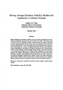
For our present work, we estimated total intensity function 𝑎(𝑡) from intertrade data allowing for intraday variation. Figure 2 is the intertrade duration histogram of our 3 NYSElisted stocks averaged over all times of the day. We divided the intertrade data into half-hour periods over the course of the day and took 𝑎 to be constant over these half-hour periods: 𝑎 (𝑡) =

Average number of trades in period 1800 seconds

(45)

for 𝑡 in that daily period. (C2) There exist some positive constants 𝛿, 𝐶 such that 𝛿 ≤ 𝑎(𝑡) ≤ 𝐶 for all 𝑡. ̂ℎ ; 𝑌) is Based on representation (40), (44), (𝑋, 𝜃, 𝜗, 𝑍 ̂ℎ ) framed by a partial-observation model, where (𝑋, 𝜃, 𝜗, 𝑍 is the state (signal), which is partially observed through the infinite dimensional counting process 𝑌. One difficulty in calibrating these models is that their transition probability functions are usually unknown in closed form, so maximum likelihood estimation (MLE) methods are difficult to use (see A¨ıt-Sahalia and Kimmel [43] for further details). Instead, we use Bayesian filtering because (1) Bayes estimates do not require the availability or regularity of the full likelihood functions; (2) Bayes estimates can be computed recursively for our tick-by-tick data; (3) Bayesian hypothesis tests can be conducted through Bayes factor, which is the ratio of marginal likelihoods and is easily computed even when the signals are of different dimension or, more generally, singular to each other.

3. Model Calibration Our foremost goal is to contribute to the process of model building for financial markets both by suggesting elements to be included in the models and proposing methods to select models based on real observation data. To be able to do this effectively, we need to be able to tune each possible model effectively to get good prior (probability distribution) ̂ℎ ) before the estimates for the complete signal (𝑋, 𝜃, 𝜗, 𝑍 test period. We do this through nonlinear filtering and in particular through particle filtering. In this section, we first


9

introduce the filtering equations for our problem. Then, we introduce a branching particle filter algorithm that is an approximation to the unnormalized filter and can be implemented on a computer. Next, we explain how we did the calibration (i.e., came up with this prior distribution) and finally we give the results for the models of interest herein.

(see Bremaud [44], p. 165) then links the desired (real-world) conditional distribution 𝜋𝑡 with the unnormalized filter 𝜎𝑡 by

3.1. Nonlinear Filtering Equations. The available information ̂ℎ ) is the observation filtration F𝑌 ⊂ F𝑡 , about (𝑋𝑡 , 𝜃, 𝜗, 𝑍 𝑡 𝑡 defined in (43), and the primary goal of nonlinear filtering is to characterize the conditional distribution

̂ℎ ) 𝐿 𝑡 | F𝑌 ] 𝜎𝑡 (𝑓) ≐ EQ [𝑓 (𝑋𝑡 , 𝜃, 𝜗, 𝑍 𝑡 𝑡

̂ℎ ) ∈ ⋅ | F𝑌 ] 𝜋𝑡 (⋅) = P [(𝑋𝑡 , 𝜃, 𝜗, 𝑍 𝑡 𝑡

(46)

or, equivalently, ̂ℎ ) | F𝑌 ] 𝜋𝑡 (𝑓) = E [𝑓 (𝑋𝑡 , 𝜃, 𝜗, 𝑍 𝑡 𝑡

(47)

̂ℎ is the for 𝑓 ∈ 𝐵(R𝑛𝑥 +𝑛𝜃 +2 × 𝐶[0, 𝑇]). Here, 𝜗 = (𝜖, 𝜙), 𝑍 long memory portion of our information noise and (𝑋, 𝜃) is the state and parameter of our fair price-volatility martingale problem. Remark 14. Actually, we often only want to estimate P[(𝑋𝑡 , 𝜃) ∈ ⋅ | F𝑌𝑡 ], but there is no simple recursive formula for this marginal. The filter is naturally model dependent, so we can produce different filtering processes for each model, that is, for each SV choice (1–5), each value of Δ, and each value of ℎ in our inertia process. Suppose 𝜅𝑧 is a positive constant for each 𝑧 ∈ N0 such that 𝜅 ≐ ∑∞ 𝑧=0 𝜅𝑧 < ∞, and consider the continuous-time likelihood function 𝐿 𝑡 = 𝐿 𝑡 (𝑋, 𝜗, 𝑍ℎ ) 󵄨 󵄨󵄨 𝑡 󵄨󵄨 𝜆 𝑧 (𝑋𝑠 , 𝜗, 𝑍𝑠ℎ , 𝑠) 󵄨󵄨󵄨 󵄨󵄨 𝑌 (𝑑𝑧, 𝑑𝑠) = exp (∫ ∫ ln 󵄨󵄨󵄨󵄨 󵄨󵄨 𝜅𝑧 󵄨󵄨 󵄨󵄨 0 𝐸 󵄨 󵄨 − ∫ (𝑎 (𝑠) − 𝜅) 𝑑𝑠) . 0

𝐿 𝑡 is a martingale under Condition (C2) and Q, defined by

=

𝐿−1 𝑇

(i.e. Q (𝐴) = ∫

𝐴

(50)

where the unnormalized filter 𝜎𝑡 is defined by (51)

for all 𝑓 ∈ 𝐵(R𝑛𝑥 +𝑛𝜃 +2 ⊗ 𝐶[0, 𝑇]). Now, we can give the evolution equation for 𝜎𝑡 . Theorem 15. Under (C1) and (C2), the unnormalized filter 𝜎𝑡 is the unique measure-valued solution of the stochastic filtering equation 𝑡

𝜎𝑡 (𝑓) = 𝜎0 (𝑓) + ∫ 𝜎𝑠 ((A − 𝑎 (𝑠) + 𝜅) 𝑓) 𝑑𝑠 0

𝑡

𝜆 (𝑠−) + ∫ ∫ 𝜎𝑠− (( 𝑧 − 1) 𝑓) 𝑌 (𝑑𝑧, 𝑑𝑠) , 𝜅𝑧 0 𝐸

(52)

for 𝑡 > 0 and 𝑓 ∈ D(A). This theorem is a modest generalization of prior results and can be obtained in much the same manner as results in Kouritzin and Zeng [23] and Xiong and Zeng [22]. Here, A is ̂ℎ ) the generator of the joint martingale problem to (𝑋, 𝜃, 𝜗, 𝑍 𝑍 obtained from A, the generator of state (𝑋, 𝜃) and A , the ̂ℎ . We do not need an generator of the historical process 𝑍 explicit formula for A. Instead, we can use particle filters to approximate 𝜎𝑡 . Henceforth, it is convenient to think of the reference measure Q as the standard measure from which we can construct the measure P𝑘,𝜃,𝜗,ℎ,Δ corresponding to model 𝑘 ∈ {1, . . . , 5} with parameters 𝜃 and microstructure with parameters 𝜗, ℎ, and Δ. 3.2. Particle Filter. The weighted filter is the simplest of particle filters. The idea behind the weighted filter is that, by the ̂ℎ ) from the observations independence of signal (𝑋, 𝜃, 𝜗, 𝑍 𝑌 under Q, we can create an infinite collection of particles 𝑘 𝑘 𝑘 ̂ℎ,𝑘 𝑁 {𝑃𝑘 }𝑁 𝑘=1 = {(𝑋 , 𝜃 , 𝜗 , 𝑍 )}𝑘=1 , each having the same law ̂ℎ ) that are also independent of the observations. as (𝑋, 𝜃, 𝜗, 𝑍 Then, it follows from the law of large numbers that for Qalmost all 𝑌 we have the weak convergence of finite measures

(49) 𝐿−1 𝑇 𝑑P

𝜎𝑡 (𝑓) , 𝜎𝑡 (1)

(48)

𝑡

𝑑Q 󵄨󵄨󵄨󵄨 󵄨 𝑑P 󵄨󵄨󵄨F𝑇

𝜋𝑡 (𝑓) =

for 𝐴 ∈ F𝑇 ) ,

is called the reference measure. Under Q, the observations are just a Poisson measure, independent of the state vector ̂ℎ ), with mean measure 𝜂(𝐴 × (0, 𝑡]) = ∑ 𝜅𝑧 × (𝑋, 𝜃, 𝜗, 𝑍 𝑧∈𝐴 (0, 𝑡]. To make the likelihoods more manageable in the particle filters to follow, we choose 𝜅 to be a long time average 𝑇 value (1/𝑇) ∫0 𝑎(𝑠)𝑑𝑠 of 𝑎(𝑠) and 𝑧 → 𝜅𝑧 to be highest where the trades will be more concentrated. Bayes Theorem

𝜎𝑡𝑁,𝑊 ≐

1 𝑁 ∑ 𝐿 (𝑋𝑘 , 𝜗𝑘 , 𝑍ℎ,𝑘 ) 𝛿(𝑋𝑘 ,𝜃𝑘 ,𝜗𝑘 ,𝑍̂ℎ,𝑘 ) 󳨐⇒ 𝜎𝑡 . 𝑡 𝑡 𝑁 𝑘=1 𝑡

(53)

Unfortunately, it is well known that the weighted particle filter may not work well for a fixed number of particles 𝑁. Roughly speaking, most of the particles diffuse away, do not track the signal well, are assigned low likelihoods, and do not really affect the average 𝜎𝑡𝑁,𝑊. Meanwhile, very few particles do match the observations better and have likelihoods that are orders of magnitude higher than of the majority of particles.

10


𝜎𝑡𝑁,𝑊 essentially becomes an average over too few particles to reflect 𝜎𝑡 well. To fix the weighted filter particle spread problem, we add particle resampling, resulting in following novel particle filter. (See Gordon et al. [45], Del Moral et al. [46], Del Moral et al. [12], and Ballantyne et al. [47] for earlier algorithms.) For some large 𝑁 ∈ N0 , the particle system {𝑃𝑘 }𝑁 𝑘=1 = ̂ℎ,𝑘 )}𝑁 is constructed as follows. {(𝑋𝑘 , 𝜃𝑘 , 𝜗𝑘 , 𝑍 𝑘=1 3.2.1. Initialization. At the initial time 𝑡0 = 0, we generate independent particles {𝑃0𝑘 }𝑁 𝑘=1 from the joint prior distribûℎ ) ∈ R𝑛𝑥 +𝑛𝜃 +2 × 𝐶[0, 𝑇]. The empirical tion 𝜋0 (⋅) of (𝑋0 , 𝜃, 𝜗, 𝑍 0 measure at 𝑡0 is

based upon (48). At the 𝑖th observation (𝑡𝑖 , 𝑌𝑡𝑖 ), the 𝑘th particle’s weight is multiplied by 𝜔𝑖𝑘 ≐ exp (∫

𝑡𝑖−1

𝑡𝑖

−∫

𝑡𝑖−1

𝑡𝑖

−∫

1 𝑁 ∑ 𝛿 𝑘 (⋅) , 𝑁 𝑘=1 𝑃0

(54)

∫ ln

𝜆 𝑧 (𝑋𝑠𝑘 , 𝜗𝑘 , 𝑍𝑠ℎ,𝑘 , 𝑠) 𝜅𝑧

𝐸

, 𝑡𝑖 ) 𝜆 𝑧𝑖 (𝑋𝑡𝑘𝑖 , 𝜗𝑘 , 𝑍𝑡ℎ,𝑘 𝑖

lim (𝜎0𝑁, 𝑓) = 𝜎0 (𝑓)

(57)

𝜅𝑧𝑖

(𝑎 (𝑠) − 𝜅) 𝑑𝑠) ≗ 𝛼𝑖 (𝑃̂𝑡𝑘𝑖 , 𝑡𝑖 , 𝑡𝑖−1 ) ,

where 𝑧𝑖 = 𝑌𝑡𝑖 . Hence, the 𝑘th particle’s weight becomes ̂ 𝑘 = 𝜔𝑘 A𝑖−1 L 𝑖 𝑖

where 𝛿𝑥 (⋅) is the Dirac measure at 𝑥. By the strong law of large numbers,

𝑌 (𝑑𝑧, 𝑑𝑠)

(𝑎 (𝑠) − 𝜅) 𝑑𝑠)

= exp (ln

𝑡𝑖−1

𝜎0𝑁 =

𝑡𝑖

(58)

and the average weight is N

A𝑖 =

1 𝑖−1 ̂ 𝑘 ∑L . 𝑁 𝑘=1 𝑖

(59)

(56)

, 𝑡𝑖 −) = (𝑋𝑡𝑘𝑖 , 𝑍𝑡ℎ,𝑘 , 𝑡𝑖 ) in (57) by continNote that (𝑋𝑡𝑘𝑖 − , 𝑍𝑡ℎ,𝑘 𝑖− 𝑖 𝑘 uous paths. Here, 𝜔𝑖 depends on the observation 𝑌 and the increment of likelihood ratio of measure P over measure Q defined by (48) given the simulated particle path realized on the interval [𝑡𝑖−1 , 𝑡𝑖 ). These weights do not depend upon the parameters 𝜃 directly. This is common and is why the observations are often called partial observations. We still can estimate 𝜃 and include these parameters as part of the particles’ states since they do affect stock price 𝑆, which is observed in the presence of noise and distortion. The weights are stored along with the states of particles before resampling.

̂ℎ is a Remark 16. When 𝐿 0 = 1, 𝜋0 (𝑓) = 𝜎0 (𝑓). Note that 𝑍 0 constant function defined on [0, 𝑇]. Whereas most particle filters approximate the filter 𝜋𝑡 , we will approximate the unnormalized filter 𝜎𝑡 to facilitate Bayesian model selection without the storage of prior filter estimates.

3.2.4. Resampling. After weighting, we resample the particles pruning the unlikely ones and duplicating the better ones ̂ 𝑘 /A𝑖 − in an unbiased manner. In particular, we let 𝜌𝑖𝑘 be (L 𝑖 𝑘 ̂ /A𝑖 ⌋)-Bernoulli random variable independent of every⌊L 𝑖 ̂ 𝑘 /A𝑖 ⌋ + 𝜌𝑘 particles at location 𝑃̂𝑘 . We thing and produce ⌊L 𝑖 𝑖 𝑡𝑖 then give all the particles weight 𝐴 𝑖 and let

𝑁→∞

∀𝑓 ∈ 𝐵 (R𝑛𝑥 +𝑛𝜃 +2 ⊗ 𝐶 [0, 𝑇]) ,

(55)

so 𝜎0𝑁 ⇒ 𝜎0 for almost all 𝑌. Here, (𝜇, 𝑓) ≐ ∫ 𝑓(𝑦)𝜇(𝑑𝑦) for measures 𝜇 so

(𝜎0𝑁, 𝑓) =

1 𝑁 ∑ 𝑓 (𝑃0𝑘 ) . 𝑁 𝑘=1

We also initialize the number of particles to N0 = 𝑁 and particle likelihoods all to A0 = 1. 3.2.2. Evolution. Between observations at 𝑡𝑖−1 and 𝑡𝑖 , the par̂ℎ,𝑘 )}N𝑖−1 , move independently as samples ticles, {(𝑋𝑘 , 𝜃𝑘 , 𝜗𝑘 , 𝑍 𝑘=1 ̂ℎ ). In particular, from the transition probability of (𝑋, 𝜃, 𝜗, 𝑍 we use the Euler scheme (see, e.g., Kloeden and Platen [48]) to evolve the dynamics, Examples 3–7 and (25). We let 𝑃̂𝑡𝑖 denote the evolved version of 𝑃𝑡𝑖−1 . 3.2.3. Particle Weights and Average Weight. We simulate using the reference measure Q and we incorporate the observations

N𝑖−1

N𝑖 ≐ ∑ {⌊ 𝑘=1

̂𝑘 L 𝑖 ⌋ + 𝜌𝑖𝑘 } . A𝑖

(60)

3.2.5. Unnormalized Filter. Now, we can estimate the unnormalized filter at the 𝑖th observation time, 𝜎𝑡𝑖 , by N𝑖

𝜎𝑡𝑁𝑖 = 𝐴 𝑖 ∑ 𝛿𝑃𝑡𝑘 . 𝑘=1

𝑖

(61)

The actual algorithm that was implemented is as follows. Initialize. {𝑃0𝑘 }𝑁 𝑘=1 are independent samples of 𝜋0 , N0 = 𝑁, N𝑛 = 0, for all 𝑛 ∈ N, and L𝑘0 = 1 for 𝑘 = 1, . . . , 𝑁.


11

Repeat. For 𝑛 = 0, 1, 2, . . ., do

$75.00

(1) evolve 𝑃𝑡𝑘𝑛 to 𝑃̂𝑡𝑘𝑛+1 independently of other particles; ̂ 𝑘 = 𝛼𝑛+1 (𝑃̂𝑘 , 𝑡𝑛+1 , 𝑡𝑛 )A𝑛 (2) weight by observation: L 𝑛+1 𝑡𝑛+1 for 𝑘 = 1, 2, . . . , N𝑛 ; 1 N𝑛 ̂ 𝑘 (3) estimate 𝜎𝑡𝑛+1 by 𝜎𝑡𝑁𝑛+1 = ∑ L 𝛿 ̂𝑘 ; 𝑁 𝑘=1 𝑛+1 𝑃𝑡𝑛+1 (4) average weight: A𝑛+1 = 𝜎𝑡𝑁𝑛+1 (1); (5) repeat: for 𝑘 = 1, 2, . . . , N𝑛 do

Bernoulli independent of everything; N +𝑗 = 𝑃̂𝑡𝑘𝑛+1 for 𝑗 = 1, . . . , N𝑘𝑛+1 ;

(b) resample: 𝑃𝑡𝑛+1𝑛+1

(c) add offspring number: N𝑛+1 = N𝑛+1 + N𝑘𝑛+1 .

Remark 17. (i) We extract our estimate before resampling to avoid excess noise. (ii) The key step is (5) that determines the new number of particles N𝑛+1 and weights L𝑘𝑛+1 in an unbiased manner. The result is zero or more particles all having the average weight at the same location as the parent. (iii) The particle evolution would typically be done via Newton’s or Milstein’s method. Since the above algorithm produces unbiased resampling of the weighted particle filter, it is quite reasonable to believe the following result. Theorem 18. Under (C1) and (C2), 𝜎𝑡𝑁𝑖 ⇒ 𝜎𝑡𝑖 for any 𝑖 and almost all observation paths. The technicality of this result’s proof would detract from our applications so it is omitted. 3.2.6. Bayesian Estimation. By Bayes rule (50), the particle approximation of the normalized filter 𝜋(⋅) is =

𝜎𝑡𝑁𝑖 (𝑓) 𝜎𝑡𝑁𝑖 (1)

$60.00 $55.00 $50.00 $45.00 $40.00 $35.00 $30.00

̂ 𝑘 /A𝑛+1 ⌋ + 𝜌𝑘 , offspring number: N𝑘𝑛+1 = ⌊L 𝑛+1 𝑛 ̂ 𝑘 /A𝑛+1 ) − ⌊L ̂ 𝑘 /A𝑛+1 ⌋)with 𝜌𝑛𝑘 being ((L 𝑛+1 𝑛+1

𝜋𝑡𝑁𝑖 (𝑓)

$65.00

(62)

for all 𝑓 ∈ 𝐵(R𝑛𝑥 +𝑛𝜃 +2 × 𝐶[0, 𝑇]). To get our parameter ̂ℎ ) to one component of estimates, we can just set 𝑓(𝑋, 𝜃, 𝜗, 𝑍 𝑖 𝑗 these parameters, that is, 𝜃 or 𝜗 . 3.3. Calibration and Historical Training. To keep the problem size manageable, we just used the clustering parameter estimates of 𝛼, 𝛽, 𝛾1 , and 𝛾2 given above as the actual values throughout our simulations. One is often faced with the problem of estimating initial distributions for fair price, volatility, and the parameters prior to filtering over the time interval of interest (April 2010 here). Our approach was to make arbitrary assignments very far in the past (January 3, 2000, to be precise) and then do an excessive amount of prior particle filtering, relying on the ability of the filter to forget its starting point and to produce

$25.00 1/3/2000 5/3/2000 9/3/2000 1/3/2001 5/3/2001 9/3/2001 1/3/2002 5/3/2002 9/3/2002 1/3/2003 5/3/2003 9/3/2003 1/3/2004 5/3/2004 9/3/2004 1/3/2005 5/3/2005 9/3/2005 1/3/2006 5/3/2006 9/3/2006 1/3/2007 5/3/2007 9/3/2007 1/3/2008 5/3/2008 9/3/2008 1/3/2009 5/3/2009 9/3/2009 1/3/2010 5/3/2010

(a)

$70.00

St∗ (with dynamics) PEP St∗ (without dynamics)

Figure 3: Long-term value estimation of PEP.

reasonable distributions at a much later point, April 1, 2010. (See, e.g., Ocone and Pardoux [49], Delyon and Zeitouni [50], and Atar [51] for mathematical results regarding this phenomenon.) This had to be done for every model, namely, every combination of our three stocks, five SV models, and multiple microstructure models, characterized by inertia parameters. Our main purpose in this historical training was ̂ℎ ) as of April to get a starting joint distribution for (𝑋, 𝜃, 𝜗, 𝑍 1, 2010, under each model combination. Due to the large number of cases this produced, we first display and discuss two models: the nondynamical microstructure Heston case and the median inertia dynamical case where ℎ = 1/2 and Δ = 7200 s (i.e., 2 hrs) in the inertia microstructure model. Also, to ensure that 𝜃 and 𝜗 did not converge to a single value, we made them vary slightly in a random manner; that is, we replaced the equation 𝑑𝜃 = 0 with 𝑑𝜃𝑡 = 𝑑V𝑡 for a very low variance Brownian motion V. In Figure 3, we illustrate our prior filtering of PepsiCo. The choppiest curve is the actual stock price while the smoothest curve is the filter’s fair price estimate 𝐸[𝑆𝑡 | F𝑌𝑡 ] using the Heston SV model with (median) microstructure inertia. The middle curve is the filter’s fair price estimate 𝐸[𝑆𝑡 | F𝑌𝑡 ] using the Heston SV model without dynamics in the microstructure; that is, 𝑍ℎ = 0. These curves go beyond April 1, 2010. However, the required initial distributions were taken from the filter at that point. Notice from Figure 3 that the implied fair price process estimate is far less volatile in the presence of dynamical microstructure than without. This lower volatility for fair price is highly desirable. It does not make sense that the fair price of a stock should fluctuate dramatically from day to day or within a day in the absence of an event, but rather these short-term fluctuations are better explained by trading noise. Moreover, fair price is a mathematically more optimal version of moving averages, which are used to judge value and momentum from, and so fair price estimates should inherit the smooth nature of such moving averages.

12

Mathematical Problems in Engineering GS: St of various models (∗ indicates models without dynamics)

Table 4 $190.00

PEP GBM HW LOU 𝜇 1.51𝐸 − 06 1.47𝐸 − 06 1.52𝐸 − 06 ] 𝜎 = 2.86𝐸 − 06 1.17𝐸 − 09 9.55𝐸 − 06 𝜅 — 1.59𝐸 − 03 1.80𝐸 − 03 󰜚 — — 4.75𝐸 − 03 𝜛 — — 4.84𝐸 − 06

Nelson 1.44𝐸 − 06 1.06𝐸 − 10 1.94𝐸 − 03 6.51𝐸 − 03 —

Heston 1.49𝐸 − 06 1.07𝐸 − 11 2.58𝐸 − 07 6.02𝐸 − 03 —

$185.00 $180.00 $175.00 $170.00 $165.00 $160.00 $155.00 $150.00 $145.00

Table 5 HW 1.02𝐸 − 06 5.50𝐸 − 10 2.18𝐸 − 03 — — 2.05𝐸 − 09 2.31𝐸 − 09

LOU 9.92𝐸 − 07 5.13𝐸 − 06 1.87𝐸 − 03 2.25𝐸 − 03 2.60𝐸 − 06 2.33𝐸 − 09 2.23𝐸 − 09

Nelson 1.03𝐸 − 06 6.32𝐸 − 11 2.12𝐸 − 03 2.90𝐸 − 03 — 2.31𝐸 − 09 2.33𝐸 − 09

4/1/2010 4/1/2010 4/5/2010 4/5/2010 4/6/2010 4/6/2010 4/7/2010 4/7/2010 4/8/2010 4/8/2010 4/9/2010 4/9/2010 4/12/2010 4/12/2010 4/13/2010 4/13/2010 4/14/2010 4/14/2010 4/15/2010 4/15/2010 4/16/2010 4/16/2010 4/19/2010 4/19/2010 4/20/2010 4/20/2010 4/21/2010 4/21/2010 4/22/2010 4/22/2010 4/23/2010 4/23/2010 4/26/2010 4/26/2010 4/27/2010 4/27/2010 4/28/2010 4/28/2010 4/29/2010 4/30/2010

$140.00

PEP GBM 𝜇 1.05𝐸 − 06 ] 𝜎 = 2.21𝐸 − 06 𝜅 — 󰜚 — 𝜛 — 𝜖 2.43𝐸 − 09 𝜙 2.13𝐸 − 09

Heston 1.01𝐸 − 06 5.94𝐸 − 12 2.26𝐸 − 07 3.23𝐸 − 03 — 2.46𝐸 − 09 2.31𝐸 − 09

From a modeling perspective, this fair price smoothness indicates that dynamical microstructure (with inertia) can replace much of what stochastic volatility tries to do and leads to one of our central questions addressed below. Is stochastic volatility necessary in the presence of dynamical microstructure?

GBM HW Log O-U GARCH Heston GBM∗

HW∗ Log O-U∗ GARCH∗ Heston∗ GS

Figure 4: Value estimation of GS, April 2010. PEP: St of various models (∗ indicates models without dynamics)

$67.00

$66.00

$65.00

$64.00

$63.00

$62.00

$61.00 4/1/2010 4/1/2010 4/1/2010 4/5/2010 4/5/2010 4/6/2010 4/6/2010 4/7/2010 4/7/2010 4/8/2010 4/8/2010 4/9/2010 4/9/2010 4/12/2010 4/12/2010 4/13/2010 4/13/2010 4/14/2010 4/14/2010 4/15/2010 4/15/2010 4/16/2010 4/16/2010 4/19/2010 4/19/2010 4/20/2010 4/20/2010 4/21/2010 4/21/2010 4/22/2010 4/22/2010 4/23/2010 4/23/2010 4/26/2010 4/26/2010 4/27/2010 4/27/2010 4/28/2010 4/28/2010 4/29/2010 4/29/2010 4/29/2010

3.4. Numerical Results. The data is one month (April 2010) of transaction prices of our three NYSE-listed stocks. Our filter produces Bayes estimates to the macro- and microparameter vectors 𝜃 and 𝜗, respectively. These estimates in the nondynamical microstructure case (i.e., using the simpler form in (24)) for PepsiCo are as shown in Table 4. All parameters are estimated using time in seconds. Our PepsiCo Bayes estimates in the median inertia case are as shown in Table 5. While it is difficult to read much from these numbers, we can see that the main volatility parameters ], 𝜅, and 󰜚 are mostly smaller when dynamics is included in the microstructure. This further justifies our conjecture that at least some stochastic volatility is better replaced by microstructure with dynamics. Figures 4 and 5 show the conditional expectation fair price estimation for Goldman Sachs and PepsiCo, respectively, in the cases of no dynamics and median inertia dynamics for each of our SV models. There are a total of eleven curves in both figures. The most volatile curve is the stock price itself over this month. The smoothest curves somewhat separated from the stock price are the fair price estimates using the five SV models with (median inertia) dynamical microstructure. The remaining five curves (that hug the stock price in Figures 4 and 5) are our fair price estimates for our five SV models with nondynamical microstructure. In this last case, the microstructure does not have the power to separate the fair price and actual stock price to any large degree.

GBM HW Log O-U GARCH Heston GBM∗

HW∗ Log O-U∗ GARCH∗ Heston∗ PEP

Figure 5: Value estimation of PEP, April 2010.

It is important to realize that these pictures are really just a one-month snapshot of a much bigger multiyear filtering process. This explains why many of the fair price processes are significantly different than the actual stock price on April 1, 2010: The filter is estimating that the difference is due to the microstructure. It is apparent that adding dynamics to the microstructure allows the estimated fair price process to differ significantly from the stock price. Indeed, there is a significant correction of all three stock prices (especially Goldman Sachs) towards estimated fair price of the models with (median inertia) dynamical microstructure. This produces a compelling reason to use models with microstructure dynamics. You would be estimating that the stocks were significantly overvalued before the correction if you used the model with microstructure dynamics and this could be


13 PEP: Zt for h = 0 versus h = 1

Table 6: Volatility estimation, April 2010. PEP (2 hrs, ℎ = 0.6) GS (1/2 day, ℎ = 0.4) IBM (1/2 day, ℎ = 1)

Without dynamics 1.58416𝐸 − 09 4.14645𝐸 − 08 8.21731𝐸 − 10

With dynamics 1.01312𝐸 − 11 4.3005𝐸 − 10 4.03211𝐸 − 11

0.08 0.07 0.06 0.05 0.04

4. Evidence for Inertia and Stochastic Volatility The main objective of this section is to use Bayes factor to investigate the model selection in microstructure markets. To use the Bayes factor method, we need only to be able to

0.03 0.02 0.01 4/1/2010 4/1/2010 4/5/2010 4/5/2010 4/6/2010 4/6/2010 4/7/2010 4/7/2010 4/8/2010 4/8/2010 4/9/2010 4/9/2010 4/12/2010 4/12/2010 4/13/2010 4/13/2010 4/14/2010 4/14/2010 4/15/2010 4/15/2010 4/16/2010 4/16/2010 4/19/2010 4/19/2010 4/20/2010 4/21/2010 4/21/2010 4/22/2010 4/22/2010 4/23/2010 4/23/2010 4/26/2010 4/26/2010 4/27/2010 4/27/2010 4/28/2010 4/28/2010 4/29/2010 4/29/2010

used as a warning to lessen ones exposure. You have no such warning when the microstructure does not contain (inertia) dynamics as the estimated fair price is very close to the observed price. It is interesting to ponder what this possible discrepancy would mean to option prices. The filters provide conditional distributions and estimates for more than just fair price and parameters. Table 6 shows the average volatility estimates without microstructure dynamics (see (24)) and with (the best performing) microstructure inertia using the simplified Heston SV model. We only highlighted Heston here because (1) we will show evidence below that Heston performs the best and (2) the volatility estimates of the other SV models behave similarly. The amount of stochastic volatility estimated when there is (median inertia) dynamics in the microstructure shrank to a couple of percent of what it was without. This really suggested that by far the primary use of stochastic volatility is as a proxy for microstructure with dynamics and further raises the question about the need for stochastic volatility in the presence of microstructure dynamics. The final and most difficult quantity the filter estimates (in the dynamical microstructure case) is the historical noise. For practical purposes, we can not let the historical path go back all the way to year 2000, but we found that there is not much loss if we just update discrete samples over the previous three years, which is still a tremendous amount of data. Also, we can not plot these historical paths so we just plot the projection onto the current time; that is, we just plot ̂ℎ 𝑍𝑡ℎ even though we must propagate the Markov process 𝑍 𝑡 in the filter. Figure 6 shows the noise estimate for PepsiCo. In this graph, we look at the effect of inertia. The curves where ℎ = 0 represent the no-inertia case, so 𝑍𝑡0 is just an OrnsteinUhlenbeck process. Conversely, the case ℎ = 1 represents the one hundred percent inertia case and 𝑍𝑡1 is not Markov. We see from these graphs that the amount of estimated noise is very similar indicating that the amount of inertia modeled might not be that significant. However, the noise processes where ℎ = 1 are far smoother due to the inertia. Below, we will produce strong evidence that inertia is important and find that the best ℎ is in the range [0.4, 1], depending upon the stock. We compare the behavior of our models in terms of the SV models and the inertia parameters ℎ and Δ within the Bayesian model selection framework in the following section.

h=0 h=1

Figure 6: Noise process estimation of PEP, April 2010.

transform all observation models of interest into the same canonical process via Girsanov measure change. The signal models can be singular to one another. Kouritzin and Zeng [23] discuss the Bayesian model selection problem. However, their equations do not apply to our models. 4.1. Model Selection and Bayes Factor. Consider our five SV macrostructure fair price-volatility models (𝑘)

𝑀(𝑘) ≐ (𝑋(𝑘) , 𝜃(𝑘) ) ∈ R𝑛𝑥

+𝑛𝜃(𝑘)

,

(63)

where the generators of the martingale problem to 𝑀(𝑘) are, respectively, A(𝑘) for 𝑘 = 1, 2, 3, 4, 5. Normally, we would have to consider a multitude of parameters 𝜃 resulting in a plethora of models. However, by our calibration process we have reduced the setting to one parameter set per martingale problem so we have a base of five models. However, we still have to consider the various choices for our inertia. For simplicity, we restrict ourselves to three distinct values for Δ, eleven choices for ℎ, and we use the calibration process to estimate the other microstructure parameters 𝜗. Therefore, we have a total of 5 × 3 × 11 = 165 models to test. The likelihood of 𝑌 being produced by model (𝑘, ℎ, Δ) up until time 𝑡 is 𝐿(𝑘,ℎ,Δ) 𝑡

𝑡

=1+∫ ∫ ( 0

𝐸

𝜆 𝑧 (𝑋𝑠(𝑘) , 𝑍𝑠ℎ,Δ , 𝜗, 𝑠) 𝜅𝑧

− 1)

(64)

(𝑌 (𝑑𝑧, 𝑑𝑠) − 𝜅𝑧 𝑚 (𝑑𝑧) 𝑑𝑠) . ⋅ 𝐿(𝑘,ℎ,Δ) 𝑠− Here, 𝑚(𝑑𝑧) is the counting measure on 𝐸 = N0 and the same observations and observation rate information are used for as the likelihood ratio of all models. One can think of 𝐿(𝑘,ℎ,Δ) 𝑡 (𝑘,ℎ,Δ) with distribution P(𝑘,ℎ,Δ) characterized by the model 𝑀 (𝑘, ℎ, Δ) to the simple (or null) model 𝑀0 with distribution Q where the observation prices just arrive according to a Poisson measure with intensity measure 𝜇(𝐴) = ∫𝐴 𝑘𝑧 𝑚(𝑑𝑧), that is, with rate independent of any macrostructure model

14


and independent of any microstructure state. In other words, (𝐿(𝑘,ℎ,Δ) )−1 = (𝑑Q/𝑑P(𝑘,ℎ,Δ) )|F𝑡 then transforms the observa𝑡 tions into the same Poisson measure with intensity measure 𝜇(𝐴) = ∫𝐴 𝑘𝑧 𝑚(𝑑𝑧) regardless of (𝑘, ℎ, Δ). Unfortunately, depends upon 𝑋𝑠(𝑘) , 𝑍𝑠ℎ,Δ , which are unknown so we 𝐿(𝑘,ℎ,Δ) 𝑡 can not select models via the likelihood.

Table 7 𝐵12 1–3 3–12 12–150 >150

4.2. Bayes Factor. The available information in microstructure market is the observation process 𝑌, which represents the cumulative transaction records throughout all tick price levels. The normalized filter 𝜋𝑡(𝑘,ℎ,Δ) , 𝑘 = 1, 2, 3, 4, 5, ℎ ∈ [0, 1], Δ > 0, satisfies

30.00

Evidence against Model 2 Barely mentionable Positive Strong Decisive PEP: 2 h and h = 0.6 Bayes with and without dynamics

25.00 20.00 15.00

𝜋𝑡(𝑘,ℎ,Δ) (𝑓𝑘 ) = (𝑘)

𝜎𝑡(𝑘,ℎ,Δ) (𝑓𝑘 ) , 𝜎𝑡(𝑘,ℎ,Δ) (1)

10.00

(65)

5.00

(𝑘)

where 𝑓𝑘 ∈ 𝐵(R𝑛𝑥 +𝑛𝜃 +2 ⊗ 𝐶[0, 𝑇]) for 𝑘 = 1, 2, 3, 4, 5, the unnormalized filter 𝜎𝑡(𝑘,ℎ,Δ) is 𝜎𝑡(𝑘,ℎ,Δ) (𝑓𝑘 ) ̂ℎ,Δ ) 𝐿(𝑘,ℎ,Δ) | F𝑌 ] , ≐ EQ [𝑓𝑘 (𝑋𝑡(𝑘) , 𝜃(𝑘) , 𝜗, 𝑍 𝑡 𝑡 𝑡

EQ [

𝑑P 𝑑Q

| F𝑌𝑡 ] = 𝜎𝑡(𝑘,ℎ,Δ) (1) ,

4/1/2010 4/1/2010 4/5/2010 4/5/2010 4/6/2010 4/6/2010 4/7/2010 4/7/2010 4/8/2010 4/8/2010 4/9/2010 4/12/2010 4/12/2010 4/13/2010 4/13/2010 4/14/2010 4/14/2010 4/15/2010 4/15/2010 4/16/2010 4/16/2010 4/19/2010 4/20/2010 4/20/2010 4/21/2010 4/21/2010 4/22/2010 4/22/2010 4/23/2010 4/23/2010 4/26/2010 4/26/2010 4/27/2010 4/28/2010 4/28/2010 4/29/2010 4/29/2010

Heston GARCH Log O-U HW GBM Heston∗

(66)

and 𝜎𝑡(𝑘,ℎ,Δ) (1) is the integrated (or marginal) likelihood of 𝑌 for model (𝑘, ℎ, Δ). Now, we use Bayes factor to compare models. The Bayes factor determines which model best fits this observed data by doing pairwise comparisons. We define Bayes factor of model 𝑀(𝑘,ℎ,Δ) to the null model by the conditional likelihood: (𝑘,ℎ,Δ)

0.00

(67)

which is consistent with more basic definitions of Bayes factor. It then follows that the Bayes factors for two models, characterized by (𝑘1 , ℎ1 , Δ 1 ) and (𝑘2 , ℎ2 , Δ 2 ), are the ratios

Figure 7: Bayes factor for PEP SV model determination, April 2010. Table 8: Bayes factor for model determination, April 2010. Heston GARCH Log O-U PEP (2 hrs, ℎ = 0.6) 27.30 25.23 21.31 GS (1/2 day, ℎ = 0.4) 19.14 18.91 18.77 IBM (1/2 day, ℎ = 1) 49.94 45.43 40.75 PEP∗ (2 hrs, ℎ = 0.6) 1.08 1.07 1.06 1.04 1.06 GS∗ (1/2 day, ℎ = 0.4) 1.06 1.04 1.06 IBM∗ (1/2 day, ℎ = 1) 1.06 ∗

𝜎1 (1) 𝐵12 (𝑡) = 𝑡2 , 𝜎𝑡 (1)

(68)

𝜎2 (1) , 𝐵21 (𝑡) = 𝑡1 𝜎𝑡 (1) (𝑘 ,ℎ ,Δ )

with the integrated likelihoods 𝜎𝑡1 (1) = 𝜎𝑡 1 1 1 (1), 𝜎𝑡2 (1) = (𝑘 ,ℎ ,Δ ) 𝜎𝑡 2 2 2 (1) that can be approximated using the algorithm of Section 3.2.5. Kass and Raftery [20] demonstrate how to interpret Bayes factor shown in Table 7. 4.3. Numerical Results on Stochastic Volatility. First, we consider the problem of selecting the best of our five fair pricevolatility models, 𝑀(𝑘) ≐ (𝑋(𝑘) , 𝜃(𝑘) ) ,

(69)

and the resulting partially observed market models, ̂ℎ,Δ , 𝜃(𝑘,ℎ,Δ) , 𝜗; 𝑌) . (𝑋(𝑘) , 𝑍

(70)

GARCH∗ Log O-U∗ HW∗ GBM∗

HW GBM 17.04 6.08 18.59 10.18 37.07 16.16 1.04 1.00 1.06 1.00 1.03 1.00

Without dynamics.

We compare these five models to determine which can best represent the market data. More precisely, we run all unnormalized filters as explained in Section 3.2 with the optimal parameters discovered and reported earlier. Then, we choose Model 𝑖 if 𝜎𝑇(𝑖,ℎ,Δ) is the largest. Naturally, this corresponds to the model whose Bayes factor ends up greater than one when compared to any other model. While we have five basic models, we also consider different market ingestion times Δ and inertia magnitude parameters ℎ for each model. Using GBM with nondynamic microstructure (i.e., 𝑍ℎ = 0) as the benchmark, we determine which combination of SV model and inertia parameters outperforms GBM most. We first focus on the candidate models (Examples 3–7). In each case, we pick the inertia parameters from the sets Δ ∈ {30 mins, 2 hrs, 1/2 day} and ℎ ∈ {0, 0.1, 0.2, . . . , 0.9, 1} that would yield the highest Bayes factor against the calibration model. The data is the transaction price of PepsiCo, IBM, and Goldman Sachs, April 2010. Figure 7 and Table 8 summarize


15

PEP: Bayes factor for Heston model with h = 0.6 (∗ indicates

models without dynamics)

30.00

PEP: Bayes Heston model with alpha: 2 h (∗ indicates models without dynamics)

30.00 25.00 25.00 20.00 20.00 15.00 15.00 10.00 10.00 5.00 5.00 4/1/2010 4/1/2010 4/1/2010 4/5/2010 4/5/2010 4/6/2010 4/6/2010 4/7/2010 4/7/2010 4/8/2010 4/8/2010 4/9/2010 4/9/2010 4/12/2010 4/12/2010 4/13/2010 4/13/2010 4/14/2010 4/14/2010 4/15/2010 4/15/2010 4/16/2010 4/16/2010 4/19/2010 4/19/2010 4/19/2010 4/20/2010 4/20/2010 4/21/2010 4/21/2010 4/22/2010 4/22/2010 4/23/2010 4/23/2010 4/26/2010 4/26/2010 4/27/2010 4/27/2010 4/28/2010 4/28/2010 4/29/2010 4/29/2010

0.00 4/1/2010 4/1/2010 4/1/2010 4/5/2010 4/5/2010 4/6/2010 4/6/2010 4/7/2010 4/7/2010 4/8/2010 4/8/2010 4/9/2010 4/9/2010 4/12/2010 4/12/2010 4/13/2010 4/13/2010 4/14/2010 4/14/2010 4/15/2010 4/15/2010 4/16/2010 4/16/2010 4/19/2010 4/19/2010 4/19/2010 4/20/2010 4/20/2010 4/21/2010 4/21/2010 4/22/2010 4/22/2010 4/23/2010 4/23/2010 4/26/2010 4/26/2010 4/27/2010 4/27/2010 4/28/2010 4/28/2010 4/29/2010 4/29/2010

0.00

40 M: h = 0.6 Heston∗

Heston∗ 2 h: h = 0.5 2 h: h = 0 2 h: h = 0.6 2 h: h = 0.1 2 h: h = 0.7

2 h: h = 0.6 1/2 day: h = 0.6

Figure 8: Bayes factor for PEP ingestion time determination, April 2010.

2 h: h = 0.2 2 h: h = 0.8 2 h: h = 0.3 2 h: h = 0.9 2 h: h = 0.4 2 h: h = 1

Figure 9: Bayes factor for PEP inertia determination, April 2010. Table 9: Bayes factor for ingestion time determination, April 2010. GS (ℎ = 0.4) PEP (ℎ = 0.6) IBM (ℎ = 1) ∗

Heston∗ 1.000 1.000 1.00

40 mins 15.083 19.066 31.152

2 hrs 17.578 25.259 42.744

1/2 day 18.100 24.187 46.988

Without dynamics.

the Bayes factor performance. The Bayes factors computed in this table give strong evidence (based upon the Kass and Raftery criterion mentioned before) for the Heston model based on a full month of real tick-by-tick stock price data. Indeed, as we will see below, there would still be strong evidence supporting Heston if we used different values of ℎ and Δ. It is also interesting that the order of the models did not change over our three stock selections, with Heston always being preferred and GBM always performing the worst. Recall that all models are tuned to have their best parameters 𝜃 and 𝜗. 4.4. Numerical Results on Inertia. Next, we look at the ingestion time Δ using nondynamic microstructure Heston as the calibration model. Figure 8 and Table 9 show the effect of varying Δ over {30 mins, 2 hrs, 1/2 day} for ℎ ∈ {0, 0.1, 0.2, . . . , 0.9, 1} fixed to give the highest Bayes factor. There is a drop in the Bayes factor values from the model determination experiment which is entirely due to the change of calibration model from GBM with nondynamic microstructure to Heston with nondynamic microstructure. Our results show that the best ingestion times for Goldman Sachs, PepsiCo, and International Business Machines stocks are, respectively, 1/2 day, 2 hours, and 1/2 day. The fact that the data supports long-time ingestion might add merit to the case of the momentum trader.

Table 10: Bayes factor for inertia determination, April 2010. ℎ ∗ 0 0.1 0.2 0.3 0.4 PEP (2 hrs) 1.00 3.745 5.875 6.950 11.693 16.733 GS (1/2 day) 1.00 11.578 13.507 16.194 17.746 18.100 IBM (1/2 day) 1.00 3.822 7.100 8.816 10.927 13.522 ℎ 0.5 0.6 0.7 0.8 0.9 1.0 PEP (2 hrs) 23.524 25.259 24.386 22.322 19.347 17.548 GS (1/2 day) 17.878 17.184 16.515 16.225 16.008 15.612 IBM (1/2 day) 16.707 20.611 25.388 31.225 38.345 46.988 ∗

Without dynamics.

Finally, we investigate the optimal amount of inertia. Figure 9 and Table 10 show the effect of varying the amount of inertia ℎ over {0, 0.1, 0.2, . . . , 0.9, 1} for Δ ∈ {30 mins, 2 hrs, 1/2 day} fixed to give the highest Bayes factor. The table shows that inertia is important. In fact, the best ℎ was always at least ℎ = 0.4 and was even ℎ = 1 in the case of IBM so all microstructure dynamics should be driven by the inertia process.

5. Conclusions Herein, we considered five popular SV models to represent intrinsic or fair price and stochastic volatility of this price. These SV models are free of inertia or momentum. We then added microstructure noise with possible dynamics and inertia to these SV models to accommodate trading noise, trend following, information dispersion, and the slow unwinding of big positions. We used Bayesian model selection techniques to determine which of these combined models fits real NYSE data best. In the process of selecting the best model we also investigated characteristics like microstructure

16


dynamics, inertia, and stochastic volatility. For the stock data considered, we can conclude the following: (1) Bayesian model selection through particle filtering provides a computationally effective means to identify the best finance models on real tick-by-tick data. (2) The SV and inertia components of the financial models compared can be singular to each other as long as the microstructure can be changed into the same canonical Poisson measure process for all models considered. (3) There is strong evidence of dynamical microstructure noise. (4) Adding dynamics to the microstructure allowed much greater deviations of price from intrinsic value, which can be detected by filtering and used as a warning sign to investors and traders. (5) The simplified Heston stochastic volatility model with microstructure dynamics and significant inertia performed the best in all cases. (6) There is strong statistical evidence that such simplified Heston stochastic volatility models with microstructure dynamics and inertia match the data better than the classical geometrical Brownian motion. (7) The amount of inertia ℎ and the time it lasted Δ varied a little from stock to stock but in all cases there was significant inertia that lasted for hours. More complicated SV models can be investigated in our future work. One could also postulate more complicated microstructure dynamics and consider additional real data analysis.

Conflict of Interests The author declares that there is no conflict of interests regarding the publication of this paper.

References [1] F. Black and M. Scholes, “The pricing of options and corporate liabilities,” Journal of Political Economy, vol. 81, no. 3, pp. 637– 654, 1973. [2] R. C. Merton, “Theory of rational option pricing,” The Bell Journal of Economics and Management Science, vol. 4, no. 1, pp. 141–183, 1973. [3] J. C. Cox, S. A. Ross, and M. Rubinstein, “Option pricing: a simplified approach,” Journal of Financial Economics, vol. 7, no. 3, pp. 229–263, 1979. [4] S. L. Heston, “A closed-form solution for options with stochastic volatility with applications to bond and currency options,” Review of Financial Studies, vol. 6, no. 2, pp. 327–343, 1993. [5] J. C. Jackwerth and M. Rubinstein, “Recovering probability distributions from option prices,” The Journal of Finance, vol. 51, no. 5, pp. 1611–1631, 1996. [6] J. Hull and A. White, “The pricing of options on assets with stochastic volatilities,” The Journal of Finance, vol. 42, no. 2, pp. 281–300, 1987.

[7] D. B. Nelson, “ARCH models as diffusion approximations,” Journal of Econometrics, vol. 45, no. 1-2, pp. 7–38, 1990. [8] B. B. Mandelbrot, Fractals and Scaling in Finance: Discontinuity, Concentration, Risk, Springer, 1997. [9] A. Shiryaev, Essentials of Stochastic Finance, World Scientific, 1999. [10] M. Capinski and T. Zastawniak, Mathematics for Finance. An Introduction to Financial Engineering, Springer, London, UK, 2nd edition, 2011. [11] M. A. Kouritzin and Y. Zeng, “Weak convergence for a type of conditional expectation: application to the inference for a class of asset price models,” Nonlinear Analysis: Theory, Methods & Applications, vol. 60, no. 2, pp. 231–239, 2005. [12] P. Del Moral, M. A. Kouritzin, and L. Miclo, “On a class of discrete generation interacting particle systems,” Electronic Journal of Probability, vol. 6, pp. 1–26, 2001. [13] R. F. Engle, “The econometrics of ultra-high-frequency data,” Econometrica, vol. 68, no. 1, pp. 1–22, 2000. [14] F. Black, “Noise,” Journal of Finance, vol. 41, pp. 529–543, 1986. [15] L. K. C. Chan and J. Lakonishok, “Institutional trades and intraday stock price behavior,” Journal of Financial Economics, vol. 33, no. 2, pp. 173–199, 1993. [16] J. Hasbrouck, Handbook of Statistics, vol. 14 of Modelling Market Microstructure Time Series, North-Holland, Amsterdam, The Netherlands, 1996. [17] J. Hasbrouck, “Security bid/ask dynamics with discreteness and clustering: simple strategies for modeling and estimation,” Journal of Financial Markets, vol. 2, no. 1, pp. 1–28, 1999. [18] R. F. Engle and J. R. Russell, “Autoregressive conditional duration: a new model for irregularly spaced transaction data,” Econometrica, vol. 66, no. 5, pp. 1127–1162, 1998. [19] F. M. Bandi and J. R. Russell, “Separating microstructure noise from volatility,” Journal of Financial Economics, vol. 79, no. 3, pp. 655–692, 2006. [20] R. E. Kass and A. E. Raftery, “Bayes factor and model uncertainty,” Journal of the American Statistical Association, vol. 90, pp. 773–795, 1995. [21] Y. Zeng, “A partially observed model for micromovement of asset prices with bayes estimation via filtering,” Mathematical Finance, vol. 13, no. 3, pp. 411–444, 2003. [22] J. Xiong and Y. Zeng, “A branching particle approximation to a filtering micromovement model of asset price,” Statistical Inference for Stochastic Processes, vol. 14, no. 2, pp. 111–140, 2011. [23] M. A. Kouritzin and Y. Zeng, “Bayesian model selection via filtering for a class of micro-movement models of asset price,” International Journal of Theoretical and Applied Finance, vol. 8, no. 1, pp. 97–121, 2005. [24] D. W. Stroock and S. R. S. Varadhan, Multidimensional Diffusion Processes, Springer, Berlin, Germany, 1979. [25] S. N. Ethier and T. G. Kurtz, Markov Processes: Characterization and Convergence, John Wiley & Sons, New York, NY, USA, 1986. [26] L. O. Scott, “Option pricing when the variance changes randomly: theory, estimation, and an application,” The Journal of Financial and Quantitative Analysis, vol. 22, no. 4, pp. 419–438, 1987. [27] F. C. Drost and B. J. M. Werker, “Closing the GARCH gap: continuous time GARCH modeling,” Journal of Econometrics, vol. 74, no. 1, pp. 31–57, 1996. [28] R. J. Elliott, W. P. Malcolm, and A. H. Tsoi, “Robust parameter estimation for asset price models with Markov modulated


[29]

[30]

[31]

[32]

[33]

[34]

[35]

[36]

[37]

[38]

[39]

[40]

[41]

[42]

[43]

[44] [45]

[46]

volatilities,” Journal of Economic Dynamics and Control, vol. 27, no. 8, pp. 1391–1409, 2003. D. Duffie, J. Pan, and K. Singleton, “Transform analysis and asset pricing for affine jump-diffusions,” Econometrica, vol. 68, no. 6, pp. 1343–1376, 2000. B. Eraker, M. Johannes, and N. Polson, “The impact of jumps in volatility and returns,” The Journal of Finance, vol. 58, no. 3, pp. 1269–1300, 2003. B. Eraker, “Do stock prices and volatility jump? Reconciling evidence from spot and option prices,” The Journal of Finance, vol. 59, no. 3, pp. 1367–1403, 2004. P. R. Hansen and A. Lunde, “Realized variance and market microstructure noise,” Journal of Business and Economic Statistics, vol. 24, no. 2, pp. 127–161, 2006. J.-C. Duan and A. Fulop, “Estimating the structural credit risk model when equity prices are contaminated by trading noises,” Journal of Econometrics, vol. 150, no. 2, pp. 288–296, 2009. Y. A¨ıt-Sahalia, P. Mykland, and L. Zhang, “How often to sample a continuous-time process in the presence of market microstructure noise,” Review of Financial Studies, vol. 18, pp. 351–416, 2005. N. Jegadeesh and S. Titman, “Returns to buying winners and selling losers: implications for stock market efficiency,” The Journal of Finance, vol. 48, no. 1, pp. 65–91, 1993. T. J. Moskowitz and M. Grinblatt, “Do industries explain momentum?” The Journal of Finance, vol. 54, no. 4, pp. 1249– 1290, 1999. B. D. Grundy and J. S. Martin, “Understanding the nature of the risks and the source of the rewards to momentum investing,” Review of Financial Studies, vol. 14, no. 1, pp. 29–78, 2001. J. M. Griffin, X. Ji, and J. S. Martin, “Momentum investing and business cycle risk: evidence from Pole to Pole,” Journal of Finance, vol. 58, no. 6, pp. 2515–2547, 2003. R. D. Huang and H. R. Stoll, “Tick size, bid-ask spreads, and market structure,” Journal of Financial and Quantitative Analysis, vol. 36, no. 4, pp. 503–522, 2001. K. H. Chung, B. F. Van Ness, and R. A. Van Ness, “Trading costs and quote clustering on the NYSE and NASDAQ after decimalization,” Journal of Financial Research, vol. 27, no. 3, pp. 309–328, 2004. K. H. Chung, K. A. Kim, and P. Kitsabunnarat, “Liquidity and quote clustering in a market with multiple tick sizes,” Journal of Financial Research, vol. 28, no. 2, pp. 177–195, 2005. M. J. Barclay, “Bid-ask spreads and the avoidance of odd-eighth quotes on nasdaq: an examination of exchange listings,” Journal of Financial Economics, vol. 45, no. 1, pp. 35–60, 1997. Y. A¨ıt-Sahalia and R. Kimmel, “Maximum likelihood estimation of stochastic volatility models,” Journal of Financial Economics, vol. 83, no. 2, pp. 413–452, 2007. P. Bremaud, Point Process and Queues: Martingale Dynamics, Springer, New York, NY, USA, 1981. N. J. Gordon, D. J. Salmond, and A. F. M. Smith, “Novel approach to nonlinear/non-gaussian Bayesian state estimation,” IEE Proceedings, Part F: Radar and Signal Processing, vol. 140, no. 2, pp. 107–113, 1993. P. Del Moral, J.-C. Noyer, and G. Salut, “Maslov optimisation theory: stochastic interpretation, particle resolution,” in 11th International Conference on Analysis and Optimization of Systems Discrete Event Systems, vol. 199 of Lecture Notes in Control and Information Sciences, pp. 312–318, Springer, Berlin, Germany, 1994.

17 [47] D. J. Ballantyne, H. Y. Chan, and M. A. Kouritzin, “Novel branching particle method for tracking,” in Signal and Data Processing of Small Targets, O. E. Drummond, Ed., vol. 4048 of Proceedings of SPIE, pp. 277–287, July 2000. [48] P. E. Kloeden and E. Platen, Numerical Solution of Stochastic Differential Equations, Springer, 1992. [49] D. Ocone and E. Pardoux, “Asymptotic stability of the optimal filter with respect to its initial condition,” SIAM Journal on Control and Optimization, vol. 34, no. 1, pp. 226–243, 1996. [50] B. Delyon and O. Zeitouni, “Lyapunov exponents for filtering problems,” in Applied Stochastic Analysis, M. H. A. Davis and R. J. Elliott, Eds., pp. 511–521, Gordon and Breach Science Publishers, London, UK, 1991. [51] R. Atar, “Exponential stability for nonlinear filtering of diffusion processes in a noncompact domain,” Annals of Probability, vol. 26, no. 4, pp. 1552–1574, 1998.

Advances in

Operations Research Hindawi Publishing Corporation http://www.hindawi.com

Volume 2014

Advances in

Decision Sciences Hindawi Publishing Corporation http://www.hindawi.com

Volume 2014

Journal of

Applied Mathematics

Algebra

Hindawi Publishing Corporation http://www.hindawi.com


Volume 2014

Journal of

Probability and Statistics Volume 2014

The Scientific World Journal Hindawi Publishing Corporation http://www.hindawi.com


Volume 2014

International Journal of

Differential Equations Hindawi Publishing Corporation http://www.hindawi.com

Volume 2014

Volume 2014

Submit your manuscripts at http://www.hindawi.com International Journal of

Advances in

Combinatorics Hindawi Publishing Corporation http://www.hindawi.com

Mathematical Physics Hindawi Publishing Corporation http://www.hindawi.com

Volume 2014

Journal of

Complex Analysis Hindawi Publishing Corporation http://www.hindawi.com

Volume 2014

International Journal of Mathematics and Mathematical Sciences


Journal of

Mathematics Hindawi Publishing Corporation http://www.hindawi.com

Volume 2014


Volume 2014

Volume 2014


Volume 2014

Discrete Mathematics

Journal of

Volume 2014


Discrete Dynamics in Nature and Society

Journal of

Function Spaces Hindawi Publishing Corporation http://www.hindawi.com

Abstract and Applied Analysis

Volume 2014


Volume 2014


Volume 2014

International Journal of

Journal of

Stochastic Analysis

Optimization



Volume 2014

Volume 2014