Under this scenario, to guarantee service, it is required to maximize the ...... Meritorious Service Award, the 1998 IEEE Signal Processing Society Best. Paper Award ... IEEE Signal Processing Society Distinguished Lecturer. Thomas L. ... under contracts from the U.S. Department of Defense, NASA, and Schlum- berger; he ...
IEEE TRANSACTIONS ON WIRELESS COMMUNICATIONS, VOL. 4, NO. 4, JULY 2005
1715
Min-Capacity of a Multiple-Antenna Wireless Channel in a Static Ricean Fading Environment Mahesh Godavarti, Member, IEEE, Alfred O. Hero, III, Fellow, IEEE, and Thomas L. Marzetta, Fellow, IEEE
Abstract—This paper presents the optimal guaranteed performance for a multiple-antenna wireless compound channel with M antennas at the transmitter and N antennas at the receiver on a Ricean fading channel with a static specular component. The channel is modeled as a compound channel with a Rayleigh component and an unknown rank-one deterministic specular component. The Rayleigh component remains constant over a block of T symbol periods, with independent realizations over each block. The rank-one deterministic component is modeled as an outer product of two unknown deterministic vectors of unit magnitude. Under this scenario, to guarantee service, it is required to maximize the worst case capacity (min-capacity). It is shown that for computing min-capacity, instead of optimizing over the joint density of T · M complex transmitted signals, it is sufficient to maximize over a joint density of min{T , M } real transmitted signal magnitudes. The optimal signal matrix is shown to be equal to the product of three independent matrices—a T × T unitary matrix, a T × M real nonnegative diagonal matrix, and an M × M unitary matrix. A tractable lower bound on capacity is derived for this model, which is useful for computing achievable rate regions. Finally, it is shown that the average capacity (avg-capacity) computed under the assumption that the specular component is constant but random with isotropic distribution is equal to min-capacity. This means that avg-capacity, which, in general, has no practical meaning for nonergodic scenarios, has a coding theorem associated with it in this particular case. Index Terms—Capacity, compound channel, information theory, multiple antennas, Ricean fading.
I. I NTRODUCTION
T
HE need for higher rates in wireless communications has never been greater than in the present. Due to this need and the derth of extra bandwidth available for communication, multiple antennas have attracted considerable attention [6], [7], [16], [20], [21]. Multiple antennas at the transmitter and the receiver provide spatial diversity that can be exploited to improve spectral efficiency of wireless communication systems and to improve performance. Manuscript received May 31, 2003; revised February 20, 2004; accepted May 31, 2004. The editor coordinating the review of this paper and approving it for publication is A. Saglione. This work was performed in part while M. Godavarti was a summer intern at the Mathematical Sciences Research Center, Bell Laboratories, and in part while M. Godavarti was a Ph.D. candidate at the University of Michigan. Parts of this work were presented at ISIT 2001 held in Washington, D.C., USA. M. Godavarti is with the Ditech Communications Inc., Mountain View, CA 94043 USA. A. O. Hero III is with the Department of Electrical Engineering, University of Michigan, Ann Arbor, MI 48109 USA. T. L. Marzetta is with Bell Laboratories, Lucent Technologies, Murray Hill, NJ 07974 USA. Digital Object Identifier 10.1109/TWC.2005.850261
Two kinds of models widely used for describing fading in wireless channels are the Rayleigh and Ricean models. For wireless links in Rayleigh fading environment, it has been shown by Foschini and Gans [6], [7] and Telatar [20] that with perfect channel knowledge at the receiver, for high signal-tonoise ratio (SNR), a capacity gain of min(M, N ) bits/s/Hz, where M is the number of antennas at the transmitter and N is the number of antennas at the receiver, can be achieved with every 3-dB increase in SNR. The assumption of complete knowledge about the channel might not be true in the case of fast mobile receivers and large number of transmit antennas because of insufficient training. Marzetta and Hochwald [16] considered the case when neither the receiver nor the transmitter has any knowledge of the fading coefficients. They considered a model where the fading coefficients remain constant for T symbol periods and instantaneously change to new independent realizations after that. They derived the structure of capacity achieving signals and also showed that under this model, the complexity for capacity calculations is considerably reduced. In contrast, the attention paid to Ricean fading models has been fairly limited. Ricean fading components traditionally have been modeled as independent Gaussian components with a deterministic nonzero mean [1], [4], [5], [12], [17], [19]. Farrokhi et al. [5] used this model to analyze the capacity of a MIMO channel with a specular component. They assumed that the specular component is deterministic and unchanging and unknown to the transmitter but known to the receiver. They also assumed that the receiver has complete knowledge about the fading coefficients (i.e., has knowledge about the Rayleigh component as well). They worked with the premise that since the transmitter has no knowledge about the specular component, the signaling scheme has to be designed to guarantee a given rate irrespective of the value of the deterministic specular component. They concluded that the signal matrix has to be composed of independent circular Gaussian random variables of mean 0 and equal variance to maximize the rate. Godavarti et al. [13] considered a nonconventional ergodic model for the case of Ricean fading where the fading channel consists of a Rayleigh component, modeled as in [16] and an independent rank-one isotropically distributed specular component. The fading channel is assumed to remain constant over a block of T consecutive symbol periods but take a completely independent realization over each block. They derived similar results on optimal capacity achieving signal structures as in [16]. They also established a lower bound to capacity that can be easily extended to the model considered in this paper. The model described in [13] is applicable to a mobile-wireless
1536-1276/$20.00 © 2005 IEEE
Authorized licensed use limited to: University of Michigan Library. Downloaded on May 5, 2009 at 16:05 from IEEE Xplore. Restrictions apply.
1716
IEEE TRANSACTIONS ON WIRELESS COMMUNICATIONS, VOL. 4, NO. 4, JULY 2005
link where both the direct line of sight component (specular component) and the diffuse component (Rayleigh component) change with time. In [12], Godavarti and Hero considered the standard Ricean fading model. The capacity calculated for the standard Ricean fading model is a function of the specular component since the specular component is deterministic and known to both the transmitter and the receiver. The authors established asymptotic results for capacity and conclude that beamforming is the optimum signaling strategy for low SNR, whereas for high SNR, the optimum signaling strategy is the same as that for purely Rayleigh fading channels. In this paper, we consider a quasi-static Ricean model where the specular component is nonchanging while the Rayleigh component is varying over time. The only difference between this model and the standard Ricean fading model is that in this model, the specular component is of single rank and is not known to the transmitter. We can also contrast the formulation here to that in [13] where the specular component is also modeled as stochastic and the ergodic channel capacity is clearly defined. In spite of a completely different formulation, we obtain surprisingly similar results as in [13]. Modeling the specular component to be of rank one is fairly common in the literature [14], [15], [18]. The rank of the specular component is determined by the number of direct line of sight paths between the transmitter and the receiver, which is typically much lower than the number of transmit and receive antennas leading to ill-conditioned specular components [10], [11]. Furthermore, if the distance between the transmit and receive antennas is much greater than the distance between individual antenna elements, then the rank of the specular component can only be one [3], [4]. The Ricean channel models considered in [12], [13] and in this paper are all extensions of the Rayleigh model considered in [16] in the sense that all models reduce to the Rayleigh model of [16] when the specular component goes to zero. The channel model considered here is applicable to the case where the transmitter and receiver are either fixed in space or are in motion but sufficiently far apart with a single direct path so that the specular component has single rank and is practically constant while the diffuse multipath component changes rapidly. This can be contrasted with the channel model in [13] where the specular component is changing as rapidly as the diffuse multipath component. This allows modeling the channel in [13] as an ergodic channel. On the other hand, the channel model in [12] is almost exactly the same as the model proposed in this paper except that in [12], it is assumed that there is a feedback path from the receiver to the transmitter and as a result the transmitter can be modeled to have complete knowledge of the specular component. In this paper, since the transmitter has no knowledge about the specular component, the transmitter can either maximize the worst case rate over the ensemble of values that the specular component can take or maximize the average rate by establishing a prior distribution on the ensemble. We address both approaches in this paper. Note that when the transmitter has no knowledge about the specular component, knowledge of it at the receiver makes no difference on the worst case capacity
[2]. We however assume the knowledge as it makes it easier to analyze the fading channel. Similar to [5], the specular component is an outer product of two vectors of unit magnitude that are nonchanging and unknown to the transmitter but known to the receiver. The difference between our approach and that of [5] is that in [5], the authors consider the channel to be known completely to the receiver. We assume that the receiver’s extent of knowledge about the channel is limited to the specular component. That is, the receiver has no knowledge about the Rayleigh component of the model. Considering the absence of knowledge at the transmitter, it is important to design a signal scheme that guarantees the largest overall rate for communication irrespective of the value of the specular component. This is formulated as the problem of determining the worst case capacity in Section II. This is followed by derivation of upper and lower bounds on the worst case capacity in Section III and optimum signal properties in Section IV. In Section V, the average capacity is considered instead of the worst case capacity, and it is shown that both formulations imply the same optimal signal structure and the same maximum possible rate. In Section VI, we use the results derived in this paper to compute capacity regions for some Ricean fading channels. For interested readers, we show the existence, in the Appendix, of a coding theorem corresponding to the worst case capacity for the fading model considered here.
II. S IGNAL M ODEL AND P ROBLEM F ORMULATION Let there be M transmit antennas and N receive antennas. It is assumed that the fading coefficients remain constant over a block of T consecutive symbol periods but are independent from block to block. Keeping that in mind, the channel is modeled as carrying a T × M signal matrix S over an M × N MIMO channel H, producing X at the receiver according to the model � X=
ρ SH + W M
(1)
where the elements, wtn of W are independent circular complex Gaussian random variables with mean 0 and variance 1 [CN (0, 1)]. The MIMO Ricean model for the matrix H is H = (1 − r)1/2 G + (rN M )1/2 αβ † where G consists of independent CN (0, 1) random variables and α and β are deterministic vectors of length M and N , respectively, such that α† α = 1 and β † β = 1. The parameter r, 0 ≤ r ≤ 1 denotes the fraction of the energy propagated via the specular component. r = 0 and r = 1 correspond to purely Rayleigh and purely specular fading, respectively. Irrespective of the value of r, the average variance of the elements of H is 1, that is, H satisfies E[tr{HH † }] = M · N . It is assumed that α and β are known to the receiver. Since the receiver is free to apply a coordinate transformation by postmultiplying X by a unitary matrix, without loss of generality, β can be taken to be identically equal to [1 0 . . . 0] T . We will sometimes write H as Hα to highlight the dependence of
Authorized licensed use limited to: University of Michigan Library. Downloaded on May 5, 2009 at 16:05 from IEEE Xplore. Restrictions apply.
GODAVARTI et al.: MIN-CAPACITY OF A WIRELESS CHANNEL IN A STATIC RICEAN ENVIRONMENT
H on α. G remains constant for T symbol periods and takes on a completely independent realization every T th symbol period. The problem in this section is to find the distribution p∗ (S) that attains the maximum in the following maximization defining the worst case channel capacity
1717
III. C APACITY U PPER AND L OWER B OUNDS ∗ Theorem 1: Min-capacity CH when the channel matrix H is known to the receiver but not to the transmitter is given by
� � ρ † ∗ He1 He1 = T E log det IN + CH M
(2)
C ∗ = max I ∗ (X; S) = max inf I α (X; S) p(S) α∈A
p(S)
and also to find the maximum value C ∗ . � I α (X; S) =
p(S)p(X|S, αβ † ) × log �
p(X|S, αβ † ) dS dX p(S)p(X|S, αβ † ) dS
is the mutual information between X and S when the specular def component is given by αβ † and A = {α : α ∈ C M and α† α = 1}. Since A is compact the “inf” in the problem can be replaced by “min.” For convenience, we will refer to I ∗ (X; S) as the min-mutual information and C ∗ as min-capacity. The above formulation is justified for the Ricean fading channel considered here because there exists a corresponding coding theorem that we prove in the Appendix. However, the existence of a coding theorem can also be obtained from [2, chap. 5, pp. 172–178]. The min-capacity defined above is just the capacity of a compound channel. We will use the notation in this paper to briefly describe the concept of compound channels given in [2]. Let α ∈ A denote a candidate channel. Let C ∗ = maxp(S) minα I α (X; S) and P ∗ (e, n) = maxα P α (e, n), where P α (e, n) is the maximum probability of decoding error for channel α when a code of length n is used. Then for every R < C ∗ , there exists a sequence of (2nR , n) codes such that lim P ∗ (e, n) = 0.
n→∞
It is also shown in [2, Prob. 13, p. 183] that min-capacity does not depend on the receiver’s knowledge of the channel. Hence, it is not necessary for us to assume that the specular component is known to the receiver. However, we do so because it facilitates easier computation of min-capacity and avgcapacity in terms of the conditional probability distribution p(X|S). Note that since A is unitarily invariant, it means that no preference is attached to the direction of the line of sight component and, therefore, it is intuitive to expect the optimum signal to attach no significance to the direction of the line of sight component as well. Moreover, since all α ∈ A have the same strength, it is intuitive to expect the optimum signal to be such that it generates the same mutual information irrespective of the choice of the specular component. This intuition is made concrete in the following sections.
where e1 = [1 0 . . . 0] T is a unit vector in C M . Note that e1 in (2) can be replaced by any α ∈ A without changing the answer. Proof: The idea for this proof has been taken from the proof of Theorem 1 in [20]. First note that for T > 1, given H, the channel is memoryless, and hence, the rows of the input signal matrix S are independent of � each other. That means α the mutual information I α (X; S) = T i=1 I (Xi ; Si ) where Xi and Si denote the ith row of X and S, respectively. The maximization over each term can be done separately, and it is easily seen that each term will be maximized individually for the same density on Si . That is, p(Si ) = p(Sj ) for i �= j and maxp(S) I α (X; S) = T maxp(S1 ) I α (X1 ; S1 ). Therefore, WLOG assume T = 1. Given H, the channel is an AWGN channel, therefore, capacity is attained by Gaussian signal vectors. Let ΛS be the input signal covariance. Since the transmitter does not know α, ΛS cannot depend on α and the min-capacity is given by maxΛS :tr{ΛS }≤M F(ΛS ) = maxΛS :tr{ΛS }≤M minα∈A E � � ρ † × log det IN + H α Λ S Hα M
(3)
where F(ΛS ) is implicitly defined in an obvious manner. First note that F(ΛS ) in (3) is a concave function of ΛS . (This follows from the fact that log det K is a concave function of K.) Also, F(Ψ† ΛS Ψ) = F(ΛS ) for any M × M Ψ : Ψ† Ψ = IM since Ψ† α ∈ A for any α ∈ A and G has independent identically distributed (i.i.d.) zero mean complex Gaussian entries. Let Q† DQ be the singular value decomposition (SVD) of ΛS , then we have F(D) = F(Q† DQ) = F(ΛS ). Therefore, we can choose ΛS to be diagonal. Moreover, F(Pk† ΛS Pk ) = F(ΛS ) for any permutation matrix Pk , k = 1, . . . , M !. There� ! † fore, if we choose Λ�S = (1/M !) M k=1 Pk ΛS Pk , then by concavity and Jensen’s inequality, we have 1 � � † F Pk ΛS Pk = F(ΛS ). M! M!
F (Λ�S ) ≥
k=1
Therefore, it can be concluded that the maximizing input signal covariance ΛS is a multiple of the identity matrix. It is quite obvious to see that to maximize the expression in (3), we need to choose tr{ΛS } = M or ΛS = IM , and since E log det[IN + (ρ/M )Hα† 1 Hα1 ] = E log det[IN + � (ρ/M )Hα† 2 Hα2 ] for any α1 , α2 ∈ A, (2) easily follows. By the data processing theorem, additional information at the receiver does not decrease capacity, hence, the following propositions.
Authorized licensed use limited to: University of Michigan Library. Downloaded on May 5, 2009 at 16:05 from IEEE Xplore. Restrictions apply.
1718
IEEE TRANSACTIONS ON WIRELESS COMMUNICATIONS, VOL. 4, NO. 4, JULY 2005
Proposition 1: An upper bound on the channel min-capacity when neither the transmitter nor the receiver has any knowledge about the channel is given by � � ρ † (4) He1 He1 . C ∗ ≤ T · E log det IN + M Now, we establish a lower bound. Proposition 2: A lower bound on min-capacity when the transmitter has no knowledge about H and the receiver has no knowledge about G is given by ��
� ρ ∗ (5) SS † − N E log2 det IT + (1 − r) C ∗ ≥ CH M � � ρ ∗ ≥ CH (6) − N M log2 1 + (1 − r) T . M Proof: Proof is a slight modification of the proof of Theorem 3 in [13], therefore, only the essential steps will be shown here. First note that I α (X; S) = I(X; S|α) = I(X; S, H|α) − I(X; H|S, α) = I(X; H|α) + I(X; S|H, α) − I(X; H|S, α) ≥ I(X; S|H, α) − I(X; H|S, α) where the last inequality follows from the fact that I(X; H|α) ≥ 0. Therefore C ∗ (X; S) ≥ max min [I(X; S|H, α) − I(X; H|S, α)]. p(S)
α
The lower bound is obtained by observing that the second term is the mutual information between the “input” H = † 1/2 (1 − r)1/2 G + (rN M ) αe1 , and the “output” X through the “channel” X = (ρ/M )SH + W . Since α is fixed and α and S are known at the “receiver,” the mutual information between H and X is the same as the mutual information between G and X � , where X � = X − (ρ/M )1/2 (rN M )1/2 Sαe†1 . Therefore, the second term can be evaluated, irrespective of the value of α, as �� �
ρ N E log2 det IT + (1 − r) SS † M and the first term can be maximized by choosing p(S) such that the elements of S are independent CN (0, 1) random variables. � Notice that the second term at right-hand side of the lower bound is � ��
ρ N E log2 det IT + (1 − r) SS † M instead of N E[log2 det(IT + (ρ/M )SS † )], which occurs in the lower bound derived for the model in [13]. The second term I(X; H|S) is the mutual information between the output and the channel given the transmitted signal. In other words, this is the information carried in the transmitted signal about the channel. Therefore, the second term in the lower bound can be viewed as a penalty term for using part of the available rate to learn the channel. When r = 1 or when the channel
is purely specular, it can be seen that the penalty term for training goes to zero. This makes perfect sense because the specular component is known to the receiver and the penalty for learning the specular component is zero in the current model as contrasted to the model in [13]. Combining (4) and (6) gives us the following. Corollary 1: The normalized min-capacity, Cn∗ = C ∗ /T in bits per channel use as T → ∞ is given by � � ρ † He1 He1 . Cn∗ = E log det IN + M Note that this is the same as the capacity when the receiver knows H, so that as T → ∞, perfect channel estimation can be performed. IV. P ROPERTIES OF C APACITY A CHIEVING S IGNALS In this section, the optimum signal structure for achieving min-capacity is derived. The optimization is being done under the power constraint E[tr{SS † }] ≤ T M . The results in this section theoretically establish what can be gauged intuitively. It has already been established in [16] that when the specular component is zero, the optimum signal density is invariant to unitary transformations. This is no longer true if the specular component is nonzero. However, if the set of nonzero specular components (called A in this paper), from which the worst case specular component is selected and the corresponding performance maximized, is invariant to unitary transformations, then it is natural to expect the optimum signal to be invariant to unitary transformations as well. The basic ideas for showing invariance of optimum signals to unitary transformations in this section, and also in the next, have been taken from [16]. Lemma 1: I ∗ (X; S) as a functional of p(S) is concave in p(S). Proof: First, note that I α (X; S) is a concave functional of p(S) for every α ∈ A. Let I ∗ (X; S)p(S) denote I ∗ (X; S) evaluated using p(S) as the signal density. Then I ∗ (X; S)δp1 (S)+(1−δ)p2 (S) = min I α (X; S)δp1 (S)+(1−δ)p2 (S) α∈A
� ≥ min δI α (X; S)p1 (S) + (1 − δ)I α (X; S)p2 (S) α∈A
≥ δ min I α (X; S)p1 (S) + (1 − δ) min I α (X; S)p2 (S) α∈A ∗
α∈A
∗
= δI (X; S)p1 (S) + (1 − δ)I (X; S)p2 (S) . � Lemma 2: For any T × T unitary matrix Φ and any M × M unitary matrix Ψ, if p(S) generates I ∗ (X; S), then so does p(ΦSΨ† ). Proof: 1) Note that p(ΦX|ΦS) = p(X|S), therefore, I α (X; ΦS) = I α (X; S) for any T × T unitary matrix Φ and all α ∈ A. 2) Also, Ψα ∈ A for any α ∈ A and any M × M unitary matrix Ψ. Therefore, if I ∗ (X; S) achieves its minimum
Authorized licensed use limited to: University of Michigan Library. Downloaded on May 5, 2009 at 16:05 from IEEE Xplore. Restrictions apply.
GODAVARTI et al.: MIN-CAPACITY OF A WIRELESS CHANNEL IN A STATIC RICEAN ENVIRONMENT
value at α0 ∈ A, then I ∗ (X; SΨ† ) achieves its minimum value at Ψα0 because I α (X; S) = I Ψα (X; SΨ† ) for α ∈ A and Ψ an M × M unitary matrix. Combining 1) and 2), we get the lemma. � Lemma 3: The min-capacity achieving signal distribution, p(S) is unchanged by any pre- and postmultiplication of S by unitary matrices of appropriate dimensions. Proof: It will be shown that for any signal density p0 (S) generating min-mutual information I0∗ , there exists a density p1 (S) generating I1∗ ≥ I0∗ such that p1 (S) is invariant to preand postmultiplication of S by unitary matrices of appropriate dimensions. By Lemma 2, for any pair of permutation matrices, Φ (T × T ) and Ψ (M × M ) p0 (ΦSΨ† ) generates the same min-mutual information as p(S). Define uT (Φ) to be the isotropically random unitary density function of a T × T unitary matrix Φ. Similarly, define uM (Ψ). Let p1 (S) be a mixture density given as follows � � p1 (S) =
1719
and Ψ, respectively. This means that both Θ1 Φ and Θ2 Ψ are isotropically distributed making them independent of Φ, V , and Ψ. Therefore, S1 is equal to the product of three independent matrices, a T × T unitary matrix Φ, a T × M real nonnegative matrix V , and an M × M unitary matrix Ψ. Now, it will be shown that the density p(V ) on V is unchanged by rearrangements of diagonal entries of V . There are min{M !, T !} ways of arranging the diagonal entries of V . This can be accomplished by pre- and postmultiplying V by appropriate permutation matrices PT k and PM k , k = 1, . . . , min{M !, T !}. The permutation does not change the min-mutual information because ΦPT k and ΨPM k have the same density functions as Φ and Ψ. By choosing an equally weighted mixture density for V , involving all min{M !, T !} arrangements, a higher value of min-mutual information can be obtained because of concavity and Jensen’s inequality. This new density is invariant to the rearrangements of the diagonal elements of V . �
p0 (ΦSΨ† )u(Φ)u(Ψ) dΦ dΨ. V. A VERAGE C APACITY C RITERION
It is easy to see that p1 (S) is invariant to any pre- and postmultiplication of S by unitary matrices and if I1∗ is the min-mutual information generated by p1 (S), then from Jensen’s inequality � and concavity of I ∗ (X; S), we have I1∗ ≥ I0∗ . Corollary 2: p∗ (S), the optimal min-capacity achieving signal density lies in P = ∪I>0 PI where PI = { p(S) : I α (X; S) = I
∀α ∈ A} .
(7)
Proof: This follows immediately from Lemma 3 because any signal density that is invariant to pre- and postmultiplication of S by unitary matrices generates the same mutual information � I α (X; S) irrespective of the value of α. The above result is intuitively obvious because all α ∈ A are identical to each other except for unitary transformations. Therefore, any density function that is invariant to unitary transformations is expected to behave the same way for all α. Theorem 2: The signal matrix that achieves min-capacity can be written as S = ΦV Ψ† , where Φ and Ψ are T × T and M × M isotropically distributed matrices independent of each other, and V is a T × M real nonnegative diagonal matrix, independent of both Φ and Ψ. Proof: From the SVD, we can write S = ΦV Ψ† , where Φ is a T × T unitary matrix, V is a T × M nonnegative real diagonal matrix, and Ψ is an M × M unitary matrix. In general, Φ, V , and Ψ are jointly distributed. Suppose S has probability density p0 (S) that generates min-mutual information I0∗ . Let Θ1 and Θ2 be isotropically distributed unitary matrices of size T × T and M × M independent of S and of each other. Define a new signal S1 = Θ1 SΘ†2 , generating min-mutual information I1∗ . Now conditioned on Θ1 and Θ2 , the min-mutual information generated by S1 equals I0∗ . From the concavity of the min-mutual information as a functional of p(S) and Jensen’s inequality, we conclude that I1∗ ≥ I0∗ . Since Θ1 and Θ2 are isotropically distributed, Θ1 Φ and Θ2 Ψ are also isotropically distributed when conditioned on Φ
In this section, we will investigate how much worse the worst case performance is compared to the average performance. To find the average performance, we maximize IE (X; S) = Eα [I α (X; S)], where I α is defined earlier and Eα denotes expectation over α ∈ A under the assumption that all α are equally likely. That is, under the assumption that α is unchanging over time, isotropically random and known to the receiver. Note that this differs from the model considered in [13] where the authors consider the case of a piecewise constant time varying i.i.d. specular component. Therefore, the problem can be stated as finding pE (S) the probability density function on the input signal S that achieves the following maximization CE = max Eα [I α (X; S)] p(S)
(8)
and also to find the value CE . We will refer to IE (X; S) as avg-mutual information and CE as avg-capacity. Like in the previous section, we would expect the optimum signal to be such that it generates the same mutual information irrespective of the choice of the specular component because the density function attaches no significance to any particular α ∈ A. In other words, since the set of nonspecular components A and the density function on A are such that the density function is invariant under unitary transformations, we would expect the optimum signal density to be invariant to unitary transformations as well. Moreover, since all α ∈ A are identical to each other except for unitary transformations, intuition tells us that Corollary 2 should hold here also. Therefore, the average mutual information over all α should be equal to the mutual information for a single α. That is, the average performance should be equal to the worst case performance. Formally, it will be shown that the signal density p∗ (S) that attains C ∗ also attains CE . For that, we need to establish the following lemmas. We omit some of the proofs because the proofs are very similar to the proofs in Section IV.
Authorized licensed use limited to: University of Michigan Library. Downloaded on May 5, 2009 at 16:05 from IEEE Xplore. Restrictions apply.
1720
IEEE TRANSACTIONS ON WIRELESS COMMUNICATIONS, VOL. 4, NO. 4, JULY 2005
Lemma 4: IE (X; S) is a concave functional of the signal density p(S). Lemma 5: For any T × T unitary matrix Φ and any M × M unitary matrix Ψ, if p(S) generates IE (X; S), then so does p(ΦSΨ† ). Proof: We want to show that if p(S) generates IE (X; S), then so does p(ΦSΨ† ). Now since the density function of α, p(α) = (Γ(M )/π M )δ(α† α − 1), we have IE (X; S) =
πM Γ(M )
πM = Γ(M ) =
πM Γ(M )
� �
C ∗ = CE ≥
� max
m≤M, n≤N
� I α (X; S) dα.
Note that I α (X; ΦS) = I α (X; S). Therefore � IE (X; S)
avg-capacity is also a lower bound on min-capacity and then optimizing over the number of transmit and receive antennas. Therefore
I α (X; ΦSΨ† ) dα I α (X; SΨ† ) dα.
Also note that I Ψα (X; SΨ† ) = I α (X; S), which means † I Ψ α (X; S) = I α (X; SΨ† ). Therefore � πM † � (X; S) = IE I Ψ α (X; S) dα Γ(M ) � πM = I ω (X; S) dω Γ(M ) = IE (X; S) where the last two equalities follow from the transformation ω = Ψ† α and the fact that the Jacobian of the transformation is equal to 1. � Lemma 6: The avg-capacity achieving signal distribution p(S) is unchanged by any pre- and postmultiplication of S by unitary matrices of appropriate dimensions. Corollary 3: p∗ (S), the optimal avg-capacity achieving signal density lies in P = ∪I>0 PI where PI is defined in (7). Based on the last corollary, it can be concluded that for a given p(S) in P, we have I ∗ (X; S) = minα∈A I α (X; S) = Eα [I α (X; S)] = IE (X; S). Therefore, the maximizing densities for CE and C ∗ are the same and also CE = C ∗ . Therefore, designing the signal constellation with the objective of maximizing the worst case performance is not more pessimistic than maximizing the average performance. Finally, we have the following theorem similar to Theorem 2. Theorem 3: The signal matrix that achieves avg-capacity can be written as S = ΦV Ψ† , where Φ and Ψ are T × T and M × M isotropically distributed matrices independent of each other, and V is a T × M real nonnegative diagonal matrix, independent of both Φ and Ψ. VI. N UMERICAL R ESULTS Plotting the upper and lower bounds on min-capacity leads to similar conclusions as in [13], except for the fact when r = 1, the upper and lower bounds coincide. A tighter lower bound can be obtained by first observing that a lower bound on
� � � ρ † T Eα� E log2 det In + Hα� Hα� −nE m
�� � ρ † × log2 det IT + (1 − r) Sm Sm . m
In the expression above, the expectation in the second term is over the distribution of the T × m input signal matrix Sm . The outer expectation in the first term is over the distribution of m × 1 vector α� , and the inner expectation is over the distribution of the Rayleigh component of the m × n channel matrix Hα� . Hα� is obtained from Hα by selecting the first m × n block of the original M × N channel matrix Hα . Therefore, α� is simply the vector of the first m elements of the M × 1 vector α. In Fig. 1, the min-capacity upper and lower bounds have been plotted as a function of the Ricean parameter r. It can be seen that the change in capacity is not drastic for low SNR as compared to larger SNR values. Also, from Fig. 2, we conclude that this change in capacity is more prominent for a larger number of antennas. We also conclude that for a purely specular channel, increasing the number of transmit antennas has no effect on the capacity. This is due to the fact that with a rankone specular component, only beamforming SNR gains can be exploited, no multiplexing gains are possible. VII. D ISCUSSION AND C ONCLUSION The idea of maximizing min-capacity can be traced back to [5] and [7], where intuitive arguments were used to justify the choice of identity matrix as the optimum input signal covariance matrix. In both works, the channel is assumed to be known at the receiver, hence, the optimum signal is a Gaussian signal with only its covariance matrix to be determined. Choosing the covariance matrix to be identity amounts to choosing a unitarily invariant density on the input signal. The model considered in this paper can be extended in various ways. One way would be to assume the parameter r to be not fixed. In this case, for min-capacity in addition to minimizing over α ∈ A, we would also have to minimize over the parameter r ∈ [0, 1]. For avg-capacity, the average over r needs to be taken as well, assuming a prior distribution like the uniform distribution over [0, 1] on r. In both cases, the optimum signal density would still be unitarily invariant. However, min-capacity will no longer be equal to avg-capacity. Another extension would be to assume the specular component to be composed of L rank-one components, that is H=
√
√ 1 − r G + rN M
�
1� vl αl βl† L L
l=1
�L where vl ≥ 0 with l=1 vl = 1 and αl and βl such that αl ∈ {α : α† α = 1} and βl ∈ {β : β † β = 1}. Here also, the
Authorized licensed use limited to: University of Michigan Library. Downloaded on May 5, 2009 at 16:05 from IEEE Xplore. Restrictions apply.
GODAVARTI et al.: MIN-CAPACITY OF A WIRELESS CHANNEL IN A STATIC RICEAN ENVIRONMENT
1721
Fig. 1.
Capacity upper and lower bounds as the channel moves from purely Rayleigh to purely Ricean fading. (a) ρ = 0 dB. (b) ρ = 15 dB.
Fig. 2.
Capacity upper and lower bounds as the channel moves from purely Rayleigh to purely Ricean fading. (a) ρ = 0 dB. (b) ρ = 15 dB.
optimum signal structure turns out to be unitarily invariant with CE > C ∗ . The summary of contributions in this paper is as follows. A nonergodic but tractable model for Ricean fading channel different from the one in [13] but along the lines of [5] has been proposed. For this channel, the worst case capacity was computed, and it was shown that the optimal signal structure was unitarily invariant. As a result, the optimization effort is over a much smaller set of parameters of size min{T, M }, rather than the set of size T × M which we originally began with. Since the capacity is not in closed form, a useful lower bound that illustrates the capacity trends as a function of the parameter r was derived. Finally, it was shown that the approach of maximizing the worst case scenario is not pessimistic in the sense that the signal
density maximizing the worst case performance also maximizes the average performance and the capacity value in both formulations turns out to be the same. The average capacity being equal to the worst case capacity can also be interpreted in a different manner: It has been shown that the average capacity criterion is a quality of service guaranteeing capacity.
A PPENDIX Coding Theorem for Min-Capacity To make this paper self-sufficient, we will prove the following theorem that is specific to the compound channel considered here. To understand the theorem, the reader is not required to know the material in [2].
Authorized licensed use limited to: University of Michigan Library. Downloaded on May 5, 2009 at 16:05 from IEEE Xplore. Restrictions apply.
1722
IEEE TRANSACTIONS ON WIRELESS COMMUNICATIONS, VOL. 4, NO. 4, JULY 2005
Theorem 4: For the quasi-static Ricean fading model, for every R < C ∗ , there exists a sequence of (2nR , n) codes with codewords mni , i = 1, . . . , 2nR , satisfying the power constraint such that lim sup Peα,n = 0
for any M × M unitary matrix Ψ. Second E0 [γ, p∗ (S), α] �γ � �� 1 = − log p∗ (S)p(X|S, α) 1+γ dS dX
n→∞ α
� ��
nR
where Peα,n = max2i=1 Pe (mni , α) and Pe (mi ) is the probability of incorrectly decoding the messages mi when the channel is given by Hα . Proof: Proof follows if we can show that Peα,n is bounded above by the same Gallager error exponent [8], [9] irrespective of the value of α. That follows from Lemma 7 proven at the end of this section. � The intuition behind the existence of a coding theorem is that the min-capacity C ∗ achieving signal density is such that the mutual information C ∗ between the output and the input is the same irrespective of any particular realization of the channel Hα . Therefore, any codes generated from the random coding argument designed to achieve rates up to C ∗ for any particular channel Hα achieve rates up to C ∗ for all Hα . For Lemma 7, we first need to briefly describe the Gallager error exponents [8], [9] for the quasi-static Ricean fading channel. For a system communicating at a rate R, the upper bound on the maximum probability of error is given as follows � � Peα,n ≤ exp −n max max {E0 [γ, p(S), α] − γR log 2} p(S) 0≤γ≤1
where n is the length of the codewords in the codebook used and E0 [γ, p(S), α] is as follows � �� E0 [γ, p(S), α] = − log
1
p(S)p(X|S, α) 1+γ dS
�γ dX
where S is the input to the channel and X is the observed output and p(X|S, α)
� √ √ † −1 ρ −tr [IT +(1−r) M SS † ] (X− ρrN Sαβ † )(X− ρrN Sαβ † ) e
� = ρ π T N detN IT + (1 − r) M SS † where β is simply [1 0 . . . 0] T . Maximization over γ in the error exponent yields a value of γ such that ∂E0 [γ, p(S), α]/∂γ = R. Note that for γ = 0, ∂E0 [γ, p(S), α]/∂γ = I α (X; S) [8], [9], where the mutual information has been evaluated when the input is p(S). If p(S) is the mincapacity achieving density p∗ (S), then ∂E0 [γ, p∗ (S), α]/∂γ = C ∗ . For more information, refer to [8], [9]. Lemma 7: The E0 [γ, p∗ (S), α] for the quasi-static Ricean fading model is independent of α. Proof: First, note that p∗ (S) = p∗ (SΨ† )
= − log
†
†
p (SΨ )p(X|SΨ , α) � ��
= − log
∗
∗
†
p (S)p(X|S, Ψ α)
1 1+γ
1 1+γ
�γ dS
dX
�γ dS
dX
� = E0 γ, p∗ (S), Ψ† α where the second equation follows from the fact that Ψ is a unitary matrix and its Jacobian is equal to 1 and the third equation follows from the fact that p(X|SΨ† , α)1/1+γ = p(X|S, Ψ† α)1/1+γ . Since Ψ is arbitrary, we obtain that � E0 [γ, p∗ (S), α] is independent of α. R EFERENCES [1] N. Benvenuto, P. Bisaglia, A. Salloum, and L. Tomba, “Worst case equalizer for noncoherent HIPERLAN receivers,” IEEE Trans. Commun., vol. 48, no. 1, pp. 28–36, Jan. 2000. [2] I. Csiszár and J. Körner, Information Theory: Coding Theorems for Discrete Memoryless Systems. New York: Academic, 1981. [3] H. Dai, A. F. Molisch, and H. V. Poor, “Downlink multiuser capacity of interference-limited MIMO systems,” in Proc. IEEE Int. Symp. Personal, Indoor and Mobile Radio Communications, Lisbon, Portugal, Sep. 2002, vol. 2, pp. 849–853. [4] P. F. Driessen and G. J. Foschini, “On the capacity formula for multiple input-multiple output wireless channels: A geometric interpretation,” IEEE Trans. Commun., vol. 47, no. 2, pp. 173–176, Feb. 1999. [5] F. R. Farrokhi, G. J. Foschini, A. Lozano, and R. A. Valenzuela, “Linkoptimal space–time processing with multiple transmit and receive antennas,” IEEE Commun. Lett., vol. 5, no. 3, pp. 85–87, Mar. 2001. [6] G. J. Foschini, “Layered space–time architecture for wireless communication in a fading environment when using multiple antennas,” Bell Labs Tech. J., vol. 1, no. 2, pp. 41–59, Autumn 1996. [7] G. J. Foschini and M. J. Gans, “On limits of wireless communications in a fading environment when using multiple antennas,” Wirel. Pers. Commun., vol. 6, no. 3, pp. 311–335, Mar. 1998. [8] R. G. Gallager, Information Theory and Reliable Communication. New York: Wiley, 1968. [9] ——, “A simple derivation of the coding theorem and some applications,” IEEE Trans. Inf. Theory, vol. 11, no. 1, pp. 3–18, Jan. 1965. [10] D. Gesbert, “Robust linear MIMO receivers: A minimum error-rate approach,” Signal Process., vol. 51, no. 11, pp. 2863–2871, Nov. 2003. [11] D. Gesbert, H. Bölcskei, D. A. Gore, and A. J. Paulraj, “Outdoor MIMO wireless channels: Models and performance prediction,” IEEE Trans. Commun., vol. 50, no. 12, pp. 1926–1934, Dec. 2002. [12] M. Godavarti and A. O. Hero, III, “Multiple antenna capacity in a deterministic Rician fading channel,” submitted for publication, IEEE Trans. Inf. Theory, 2001. [13] M. Godavarti, T. Marzetta, and S. S. Shitz, “Capacity of a mobile multipleantenna wireless link with isotropically random Rician fading,” IEEE Trans. Inf. Theory, vol. 49, no. 12, pp. 3330–3334, Dec. 2003. [14] J. Hansen and H. Bölcskei, “A geometrical investigation of the rank-1 Ricean MIMO channel at high SNR,” in Int. Symp. Information Theory (ISIT) 2004, Chicago, IL, p. 64. [15] S. K. Jayaweera and H. V. Poor, “On the capacity of multi-antenna systems in the presence of Rician fading,” in Proc. IEEE Vehicular Technology Conf., Vancouver, Canada, Sep. 2002, vol. 4, pp. 1963–1967. [16] T. L. Marzetta and B. M. Hochwald, “Capacity of a mobile multipleantenna communication link in Rayleigh flat fading channel,” IEEE Trans. Inf. Theory, vol. 45, no. 1, pp. 139–157, Jan. 1999. [17] S. Rice, “Mathematical analysis of random noise,” Bell Syst. Tech. J., vol. 23, pp. 282–332, Jul. 1944. [18] S. Sandhu and A. Paulraj, “Space–time block codes: A capacity perspective,” IEEE Commun. Lett., vol. 4, no. 12, pp. 384–386, Dec. 2000.
Authorized licensed use limited to: University of Michigan Library. Downloaded on May 5, 2009 at 16:05 from IEEE Xplore. Restrictions apply.
GODAVARTI et al.: MIN-CAPACITY OF A WIRELESS CHANNEL IN A STATIC RICEAN ENVIRONMENT
[19] V. Tarokh, N. Seshadri, and A. R. Calderbank, “Space–time codes for high data rate wireless communication: Performance criterion and code construction,” IEEE Trans. Commun., vol. 44, no. 3, pp. 744–765, Mar. 1998. [20] I. E. Telatar, “Capacity of multi-antenna Gaussian channels,” Eur. Trans. Telecommun., vol. 10, no. 6, pp. 585–596, Nov./Dec. 1999. [21] L. Zheng and D. N. C. Tse, “Packing spheres in the Grassmann manifold: A geometric approach to the non-coherent multi-antenna channel,” IEEE Trans. Inf. Theory, vol. 48, no. 2, pp. 359–383, Feb. 2002. Mahesh Godavarti (S’95–A’95–M’01) was born in Jaipur, India in 1972. He received the B.Tech. degree in electrical and electronics engineering from the Indian Institute of Technology, Madras, India, in 1993, and the M.S. degree in electrical and computer engineering from the University of Arizona, Tucson, AZ, in 1995. He was with the University of Michigan, Ann Arbor, MI, from 1997 to 2001, where he received the M.S. degree in applied mathematics and the Ph.D. degree in electrical engineering. Currently, he is employed as a Staff DSP Engineer with Ditech Communications, Mountain View, CA, where he is researching new algorithms for speech enhancement. His research interests include topics in speech and signal processing, communications, and information theory. Alfred O. Hero, III (S’79–M’80–SM’96–F’98) was born in Boston, MA, in 1955. He received the B.S. degree in electrical engineering (summa cum laude) from Boston University, Boston, MA, in 1980 and the Ph.D. from Princeton University, Princeton, NJ, in 1984, both in electrical engineering. While at Princeton, he held the G.V.N. Lothrop Fellowship in Engineering. Since 1984, he has been a Professor with the University of Michigan, Ann Arbor, MI, where he has appointments in the Department of Electrical Engineering and Computer Science, the Department of Biomedical Engineering, and the Department of Statistics. He has held visiting positions at I3S University of Nice, SophiaAntipolis, France, in 2001, Ecole Normale Supérieure de Lyon, Lyon, France, in 1999, Ecole Nationale Supérieure des Télécommunications, Paris, France, in 1999, Scientific Research Labs of the Ford Motor Company, Dearborn, MI, in 1993, Ecole Nationale Superieure des Techniques Avancees (ENSTA) and Ecole Superieure d’Electricite, Paris, in 1990, and Lincoln Laboratory, Massachusetts Institute of Technology, Cambridge, from 1987 to 1989. His research has been supported by NIH, NSF, AFOSR, NSA, ARO, ONR, DARPA, and by private industry in the areas of estimation and detection, statistical communications, bioinformatics, signal processing, and image processing. Dr. Hero served as Associate Editor for the IEEE TRANSACTIONS ON INFORMATION THEORY from 1995 to 1998 and again in 1999 and the IEEE TRANSACTIONS ON SIGNAL PROCESSING since 2002. He was Chairman of the Statistical Signal and Array Processing (SSAP) Technical Committee from 1997 to 1998 and Treasurer of the Conference Board of the IEEE Signal Processing Society. He was Chairman for Publicity of the 1986 IEEE International Symposium on Information Theory (Ann Arbor, MI) and General Chairman of the 1995 IEEE International Conference on Acoustics, Speech, and Signal Processing (Detroit, MI). He was cochair of the 1999 IEEE Information Theory Workshop on Detection, Estimation, Classification, and Filtering (Santa Fe, NM) and the 1999 IEEE Workshop on Higher Order Statistics (Caesaria, Israel). He chaired the 2002 NSF Workshop on Challenges in Pattern Recognition. He cochaired the 2002 Workshop on Genomic Signal Processing and Statistics (GENSIPS). He was Vice President (Finance) of the IEEE Signal Processing Society from 1999 to 2002. He was Chair of Commission C (Signals and Systems) of the U.S. National Commission of the International Union of Radio Science (URSI) from 1999 to 2002. He has been a member of the Signal Processing Theory and Methods (SPTM) Technical Committee of the IEEE Signal Processing Society since 1999. He is also a member of the SEDD Review Panel of the U.S. National Research Council. He will be President-Elect of the IEEE Signal Processing Society from 2004 to 2005. He is a member of Tau Beta Pi, the American Statistical Association (ASA), the Society for Industrial and Applied Mathematics (SIAM), and the U.S. National Commission (Commission C) of URSI. He received the 1998 IEEE Signal Processing Society Meritorious Service Award, the 1998 IEEE Signal Processing Society Best Paper Award, and the IEEE Third Millenium Medal. In 2002, he was appointed IEEE Signal Processing Society Distinguished Lecturer.
1723
Thomas L. Marzetta (S’76–M’77–SM’93–F’03) was born in Washington, D.C. He received the Ph.D. in electrical engineering from the Massachusetts Institute of Technology, Boston, MA, in 1978. His dissertation extended the three-way equivalence of autocorrelation sequences, minimum-phase prediction error filters, and reflection coefficient sequences to the two-dimensional case. He worked for Schlumberger-Doll Research from 1978 to 1987 to modernize geophysical signal processing for petroleum exploration. From 1987 to 1995, he performed research and development at Nichols Research Corporation under contracts from the U.S. Department of Defense, NASA, and Schlumberger; he headed a group that improved automatic target recognition, radar signal processing, and video motion detection. Since 1995, he has been with Bell Laboratories (formerly AT&T, now Lucent Technologies), currently in the Mathematical Sciences Research Center where he heads the Mathematics of Communications Research Department. He specializes in multiple antenna wireless with particular emphasis on techniques for realizing extremely high throughputs with large numbers of antennas. Dr. Marzetta was a member of the Sensor Array and Multichannel Technical Committee of the IEEE Signal Processing Society (2000–2003), and he has served as associate editor for two IEEE journals, and as guest associate editor for the IEEE TRANSACTIONS ON SIGNAL PROCESSING Special Issue on Signal Processing Techniques for Space–Time Coded Transmissions (Oct. 2002) and for the IEEE TRANSACTIONS ON INFORMATION THEORY Special Issue on Space–Time Transmission, Reception, Coding and Signal Design (Oct. 2003). He was the recipient of the 1981 ASSP Paper Award from the IEEE Signal Processing Society.
Authorized licensed use limited to: University of Michigan Library. Downloaded on May 5, 2009 at 16:05 from IEEE Xplore. Restrictions apply.