Annals of Operations Research manuscript No.
(will be inserted by the editor)
MineLib: A Library of Open Pit Mining Problems Daniel Espinoza · Marcos Goycoolea · Eduardo Moreno · Alexandra Newman
Received: November 11, 2014/ Accepted: –
Abstract Similar to the mixed-integer programming library (MIPLIB), we present
a library of publicly available test problem instances for three classical types of open pit mining problems: the ultimate pit limit problem and two variants of open pit production scheduling problems. The ultimate pit limit problem determines a set of notional three-dimensional blocks containing ore and/or waste material to extract to maximize value subject to geospatial precedence constraints. Open pit production scheduling problems seek to determine when, if ever, a block is extracted from an open pit mine. A typical objective is to maximize the net present value of the extracted ore; constraints include precedence and upper bounds on operational resource usage. Extensions of this problem can include (i) lower bounds on operational resource usage, (ii) the determination of whether a block is sent to a waste dump, i.e., discarded, or to a processing plant, i.e., to a facility that derives salable mineral from the block, (iii) average grade constraints at the processing plant, and (iv ) inventories of extracted but unprocessed material. Although open pit mining problems have appeared in academic literature dating back to the 1960s, no standard representations exist, and there are no commonly available corresponding data sets. We describe some representative open pit mining problems, briefly mention related literature, and provide a library consisting of mathematical models and sets of instances, available on the Internet. We conclude with directions for use of this newly established mining library. The library serves not only as a suggestion of standard expressions of and available data for open pit mining problems, but also as encouragement for the development of increasingly sophisticated algorithms. Daniel Espinoza E-mail:
[email protected] Department of Industrial Engineering, Universidad de Chile Marcos Goycoolea E-mail:
[email protected] School of Business, Universidad Adolfo Iba˜ nez Eduardo Moreno E-mail:
[email protected] Faculty of Engineering and Sciences, Universidad Adolfo Iba˜ nez Alexandra Newman E-mail:
[email protected] Division of Economics and Business, Colorado School of Mines, Golden, CO 80401
2
D. Espinoza, M. Goycoolea, E. Moreno and A. Newman
Keywords: mine scheduling, mine planning, open pit production scheduling, sur-
face mine production scheduling, problem libraries, open pit mining library 1 Introduction Mining is the process of extracting a naturally occurring material from the earth
to derive profit. Operations research has been used extensively in mining to plan when and how to perform both surface and underground extraction; decisions entail how to recover and treat the extracted material, which is (i) metallic ores such as iron and copper, (ii) nonmetallic minerals such as sand and gravel, and (iii) fossil fuels such as coal. Mining has five stages: (i) prospecting, or discovering a mineral deposit; (ii) exploration (including resource modeling), or determining the value of the deposit via estimation and simulation techniques, e.g., Krige (1951) and Deutsch (2004); (iii) development, i.e., obtaining land rights and stripping topsoil from the deposit; (iv ) exploitation, i.e., extracting the material; and (v ) reclamation, i.e., restoring the mined area to an environmentally acceptable state. Operations research has been used in mining, primarily for the development and exploitation stages. Studies evaluate the economic potential of a project, considering factors such as the size, shape, and location of the deposit, the mining method (e.g., open pit or underground), the deposit’s estimated ore content, estimated market prices, and the rate of ore extraction. Near-optimal long-range operational mine plans improve the economic viability of the project, or allow prospectors to turn their attention to more economical deposits as soon as possible (Lee 1984). If the project progresses, more detailed operational designs provide mine planners with specific extraction schedules at various levels of detail, e.g., monthly or yearly. These operational plans suggest the sequence of extraction for notional threedimensional blocks containing estimated (deterministic) amounts of ore and waste. Large excavators and haul trucks extract and subsequently transport the material to a processing plant or to an intermediate site (e.g., a mill, a leachpad, a stockpile), or to a waste dump, depending on the expected profitability of the material and processing-plant capacity. The rate at which the material is excavated and processed depends on initial capital expenditure decisions regarding purchasing equipment such as haul trucks, loaders, and processing plants, and installing infrastructure such as roads and rail lines. Processed ore can be sold according to long-term contracts or on the spot market. Waste is left in piles, which must ultimately be reclaimed when the deposit is closed. The rate at which material can be extracted from the deposit is governed by production constraints, while the rate at which it can be sent through a processing plant is governed by processing constraints. Figure 1 depicts a deep surface mine that is typical of hardrock-metal deposits containing copper or fossil fuel deposits containing coal. Overburden (i.e., waste) must be removed before extraction can begin. Haul roads wind up through the mine from the bottom of the pit to the surface. Extraction occurs from benches, which are the floors from which material is mined. The purpose of our paper is three-fold: (i) to introduce the reader to classical operational mine planning problems whose solutions support design and scheduling in the development and exploitation phases of an open pit mining project; (ii) to describe and provide data sets for variants of these problems on which researchers
Minelib
3
Fig. 1 Schematic illustration of an open-pit mine. (Source: http://visual.merriamwebster.com/energy/geothermal-fossil-energy/coal-mine/open-pit-mine.php).
can test existing and new algorithms using open-source data; and (iii) to encourage researchers to develop new, more accurate models and increasingly sophisticated algorithms to solve three types of open pit mining problems: the ultimate pit limit problem and two kinds of open pit block sequencing problems. This paper follows in the tradition of publicly available problem instances, beginning with NETLIB (Gay 1985), OR-Library (Beasley 1990), TSPLIB (Reinelt 1991), and MIPLIB (Bixby et al 1992), all of which have spurred research interest in their respective fields. In the remainder of this section, we give background on open pit mining operations, and explain constructs relevant for the optimization models we pose in our paper; we then describe the purpose of our mining library. The subsequent sections of this paper are organized as follows: In Section 2, we provide a brief overview of academic work on open pit mining problems. We give a mathematical description of three types of open pit mining problems in Section 3. Section 4 details data instances, including the format for numerical values used. Section 5 concludes with current numerical results for open pit production scheduling problems. We give the file format specifications in an appendix.
1.1 Background A common construct in open pit mining problems is the notion of spatial reference points called blocks. Geometric sequencing constraints (see Figure 2 and Figure 3) ensure that the pit walls are stable and that the equipment can access the areas to be mined. These precedence constraints ensure that blocks immediately affecting a given block’s ability to be mined are extracted before the given block is extracted. The relationship between block precedences is clearly transitive, i.e., if block a requires block b to be extracted, and block b requires block c to be extracted, then block a also requires block c to be extracted; this transitivity is implied by the original precedences. We can use this transitivity property to describe a precedence relationship as immediate if it is not implied by any other pair
4
D. Espinoza, M. Goycoolea, E. Moreno and A. Newman
Fig. 2 Sequencing rules can be based, for example, on the removal of five blocks above a given block, block 6 (left) or on the removal of nine blocks above a given block, block 10 (right).
Fig. 3 Sequencing approximation based on the removal of all blocks at a 45-degree angle above a given block, for three, eight and thirty levels
of precedences, allowing us to model precedence constraints simply by enforcing immediate precedences in our models. These sequencing rules can be thought of as approximations in strategic planning models to those used for tactical production scheduling. For example, if all the blocks on top of block number 10 in Figure 2 are removed, block 10 could be still surrounded by eight blocks on its level, rendering the extraction of block 10 either extremely costly or impossible. In fact, “blocks” do not exist in practical mining operations. They simply serve as modeling tools to discretize the orebody. The units, sometimes termed “smallest mining units,” that are used for scheduling purposes, must be representative of the mining operation being modeled. (See, for example, Askari-Nasab et al (2011) who present descriptions of and formulations for suitable block sizes.) For production scheduling at the tactical level, one may more realistically use aggregated blocks to fit the geology of the operation and the time fidelity of the model; Tabesh and Askari-Nasab (2011) present a clustering algorithm based on a similarity index to aggregate blocks into these smallest mining units. While Figure 2 may adequately represent sequencing in a “flat” mine such as a limestone quarry or a bauxite mine, very complex sequencing rules may be required, especially in underground operations (see, e.g., O’Sullivan and Newman (2012)) (Brickey 2012). Ultimately, we present the precedence format in our library in a very general way such that the user may specify any set of blocks as predecessors of a given block. The open pit production scheduling problem, whose variants we subsequently mathematically define as (CPIT ) and (PCPSP ), seeks to determine when, if ever, to mine each block in the deposit and what to do with each block that is extracted, i.e., send it to a particular type of processing plant or to the dump. The objective is to maximize the net present value gained from the extracted material subject to spatial precedence constraints, and to various operational constraints.
Minelib
5
The simplest variant of this problem might only contain a single (upper bound) operational resource constraint, i.e., a production (or extraction) upper bound. More complicated variants possess multiple operational resource constraints, e.g., processing limits, lower bound operational resource constraints, inventory balance, and/or blending requirements. We introduce a simplified version of the production scheduling problem that details the shape of the final pit, or part of the mine design. The ultimate pit limit problem, which we later mathematically define as (UPIT ), takes as given an undiscounted value for each block in a deposit; this value is based on a selling price, an estimated quantity of ore and waste contained in each block, the corresponding costs associated with block extraction, and, if applicable, processing. The model then determines the pit boundary to maximize undiscounted ore value. This problem balances the ore-to-waste (stripping) ratio with the cumulative value of blocks in the pit boundaries. The ultimate pit limit problem ignores the dimension of time, and, hence, the time value of money. Omissions due to the lack of a temporal aspect include operational resource constraints, ore blending constraints, and stockpiling considerations. The problem also assumes that the cutoff grade, i.e., the grade that separates ore from waste, is fixed. The assumption is that blocks above a threshold ratio of ore to total tonnage are sent to a processing plant, whereupon value (based on selling price less extraction and processing costs) is derived from the block, while those whose ratio falls below the threshold are sent to the dump, whereupon a cost is incurred from having extracted the block. Open-pit mine design, in design problems more general than (UPIT ), also includes the location and type of haulage ramps and additional infrastructure, as well as long-term decisions regarding the size and location of production and processing facilities.
1.2 Traditional and current solution methodologies The solution of various instances of the ultimate pit limit problem, differentiated by price, results in a series of nested pits; a given (notional) selling price for the ore defines the smallest pit and increasing ore prices define larger, economically viable pits. Traditional open-pit production scheduling groups the nested pits within the ultimate (or largest) pit into pushbacks, where a single pushback is often associated with similar operational resource usage, e.g., extraction equipment. Within each pushback (which contains only a small subset of the overall number of blocks within the block model), an extraction sequence is then determined. Among pushbacks, an extraction sequence is also delineated. Depending on the homogeneity of the material being extracted and the time fidelity of the model, blocks in some pushbacks may be extracted before all blocks in a previously started pushback have been mined. The basic premise of this approach is that one can determine a cutoff grade policy to maximize net present value (NPV) subject to capacity and other operational constraints. Higher cutoff grades in the initial years of the project lead to higher overall NPVs; over the life of the mine, the tendency is to reduce the cutoff grade to a break-even level. Lane (1988), Fytas et al (1987), and Kim and Zhao (1994), among others, address cutoff grades. Three problematic aspects of this approach can be (i) the assumption of a fixed cutoff grade, which depends on an arbitrary delineation between ore and waste; (ii) the use of notional (and monotonically increasing) prices to construct arbitrarily
6
D. Espinoza, M. Goycoolea, E. Moreno and A. Newman
defined nested pits or pushbacks; and (iii) the piecemeal approach to the entire optimization problem, which disregards the temporal interaction of operational resource requirements. Naturally, this can lead to suboptimal solutions to the production scheduling problem. More recently, hardware, software, and algorithmic developments have allowed instances of (CPIT ) and (PCPSP ) to be solved as a monolithic problem. The corresponding models possess binary variables that determine whether or not a given block is mined in a certain time period. In some cases, additional (continuous) variables indicate the amount of a block sent to a particular destination in a certain time period. The objective maximizes net present value. The constraints, generally linear, reflect the definition of the production scheduling problem. Many open pit mines are discretized into tens of thousands, or even millions of blocks. The ultimate pit limit problem can be viewed as a maximum closure problem (Lerchs and Grossmann 1965), and fast solution techniques currently solve even the largest instances well. However, the open pit production scheduling problem and its variants possess only an underlying network structure, i.e., they are not network flow problems in and of themselves. This problem and its variants not only account for time, which increases the number of variables dramatically, but also possess complicating side constraints to incorporate restrictions such as minimum and maximum operational resource usage per time period; model instances usually contain between 10 and 20 time periods although some instances, e.g., those that consider time fidelity finer than a year, can contain as many as 100 time periods. Corresponding problem instances contain millions or tens of millions of binary variables and hundreds of thousands, or even millions, of constraints.
2 Literature Review
The seminal work of Lerchs and Grossmann (1965) provides an exact and computationally tractable (network-based) method for solving the ultimate pit limit problem; Underwood and Tolwinski (1998) and Hochbaum and Chen (2000), Hochbaum (2001), and Chandran and Hochbaum (2009), among others, extend this work. However, a solution to the ultimate pit limit problem specifies only the economic envelope of profitable blocks given pit-slope requirements, and necessitates that the revenue associated with the extraction of a block is fixed a priori. Furthermore, the problem ignores the time aspect of the production scheduling problem, and, hence, the associated operational resource constraints. The ultimate pit limit problem is fairly well defined. However, the production scheduling problem has many variants, all of which contain precedence constraints, as the ultimate pit limit model does. In addition to these constraints, production scheduling problem variants possess at least one upper limit on an operational resource constraint, and may accommodate one or more of the following considerations: (i) blending, (ii) lower bounds on production, (iii) lower bounds on processing, (iv ) upper bounds on production, (v ) upper bounds on processing, (vi) inventory, and/or (vii) variable cutoff grade. (Note that this terminology is a misnomer: A variable cutoff grade implies that the grade at which a block is classified as ore is allowed to vary based on the block and time period; however, this situation is better expressed as “no cutoff grade.”) In describing the open pit production scheduling models below, we mention those aspects that the models include.
Minelib
7
The earliest work that addresses sequencing together with operational resource constraints, i.e., the production scheduling problem, is perhaps found in Johnson (1969), who proposes a very general linear program to maximize net present value subject to sequencing and operational resource constraints; he allows for a variable cutoff grade and proposes Dantzig-Wolfe decomposition to solve model instances. Because of the state of hardware and software at the time, he illustrates only small examples. Early computational work relies on the following simplifications: (i) blocks are aggregated into strata, e.g., Busnach et al (1985), Klingman and Phillips (1988), and Gershon and Murphy (1989); (ii) binary block extraction decisions are relaxed to be continuous, e.g., Tan and Ramani (1992), Fytas et al (1993); and/or (iii) the monolithic problem is addressed in stages, e.g., Sundar and Acharya (1995), Sevim and Lei (1998). Heuristics, e.g., genetic algorithms, also appear in the literature, e.g., Denby and Schofield (1994), Zhang (2006), though the examples tested are small. Caccetta and Hill (2003) provide an exact approach to solving a monolithic production scheduling problem by defining variables representing whether a block is mined by time period t. The model contains precedence constraints, as well as operational resource constraints, processing plant grade constraints, and inventory balance constraints; they use a fixed cutoff grade. The authors use a branch-andcut strategy combined with a heuristic to solve model instances. Ramazan (2007) assumes a fixed cutoff grade, and includes upper and lower bounds on processing, and upper bounds on production. He also includes a grade constraint. The author constructs aggregate “fundamental trees” to reduce the size of his production scheduling problem. Researchers have used Lagrangian Relaxation, e.g., Dagdelen and Johnson (1986), in order to maximize net present value subject to constraints on production and processing. Akaike and Dagdelen (1999) extend this work by iteratively altering the values of the Lagrangian multipliers until the solution to the relaxed problem meets the original side constraints, if possible. Kawahata (2006) includes a variable cutoff grade. This research has been successful at solving some instances, though authors also report difficulty in obtaining convergence, or even determining a feasible solution for the monolithic problem. In addition to Lagrangian Relaxation, authors develop heuristics to generate good, feasible integer solutions. Amaya et al (2009) assume a fixed cutoff grade and impose upper bound constraints on production and processing. The authors develop a random, local search heuristic that seeks to improve on an incumbent solution by iteratively fixing and relaxing part of the solution, and that produces solutions for the largest model instances solved to date, i.e., containing as many as four million blocks and 15 time periods. Given the size and complexity of production scheduling problems, researchers realize that the ability to solve the associated linear programming relaxation without the use of the simplex method is fundamental to solving corresponding largescale integer programs. The following authors exploit this idea: Boland et al (2009) propose an aggregation scheme for their production scheduling model, which assumes a variable cutoff grade and possesses upper bound constraints on production and processing. The authors introduce aggregates of blocks grouped by precedence and use this construct to approximate a solution for the original, mixed integer program. Gleixner (2008) extends results from this model variant with a different type of aggregation and also presents ideas for using Lagrangian Relaxation in
8
D. Espinoza, M. Goycoolea, E. Moreno and A. Newman
this context. Askari-Nasab et al (2010) present two formulations which rely on the construct of a “mining-cut”; this construct helps to aggregate blocks appropriately. While one of the authors’ formulations relies solely on mining-cuts, the other uses both blocks and mining-cuts. The advantage of the latter formulation is more accurate modeling of pit slopes, while the former formulation contains fewer variables and is therefore more tractable. Chicoisne et al (to appear) propose a new algorithm to solve linear programming relaxations of large instances of the same problem, and a set of heuristics to solve the corresponding integer program. The related algorithms of Bienstock and Zuckerberg (2010) include the decision of whether the extracted material should be sent to a processing plant or to the waste dump, i.e., they include a variable cutoff grade. Osanloo et al (2008) review optimization models for long-term, open-pit scheduling. See Newman et al (2010) for a detailed literature review covering both open pit and underground mine planning. In this paper, we focus specifically on mining applications. However, the structure of our problem variants is related to that of other network models with side constraints, e.g., generalized assignment, multicommodity flow, and constrained shortest path. See, e.g., Ahuja et al (1993), Carlyle et al (2008), and the references contained therein.
3 Model Description
We proceed to set forth three mathematical models relevant to open pit mining. In Subsection 3.1, we give notation for all three models. Script letters represent set names, while upper- and lower-case letters in Roman font denote parameters; standard lower-case letters of x and y serve as our variables. Parameter and variable names decorated with hats or tildes correspond to related notation that differs by index depending on the model formulation in which it is used. Subsection 3.2 describes the ultimate pit limit problem. Subsection 3.3 gives the constrained pit limit problem. Finally, Subsection 3.4 introduces the precedence constrained production scheduling problem. Subsections 3.5 and 3.6 provide a discussion regarding the strength of the formulation and modeling implications for the three models we set forth, respectively.
3.1 Notation • Indices and sets: ? t ∈ T : set of time periods t in the horizon. ? b ∈ B: set of blocks b. ? b0 ∈ Bb : set of blocks b0 that are predecessor blocks for block b. ? r ∈ R: set of operational resource types r. ? d ∈ D: set of destinations d. • Parameters: ? pb (ˆ pbt , pˇbd , p˜bdt ): profit obtained from extracting (and processing) block b (at time period t and/or sending it to destination d) ($). ? α: discount rate used in computing the objective function (profit) coeffi-
cients.
Minelib
9
? qbr (ˆ qbrd ): the amount of operational resource r used to extract and, if applicable, process, block b (when sent to destination d) (tons). ? Rrt : minimum availability of operational resource r in time period t (tons). ? Rrt : maximum availability of operational resource r in time period t (tons). ? A: arbitrary constraint coefficients on general side constraints. ? a, a ¯: arbitrary lower and upper bounds, respectively, on general side constraints (vectors with the number of rows equal to that in A). • Variables: ? x ˆb = 1 if block b is in the final pit design, 0 otherwise. ? xbt : 1 if we extract block b in time period t, 0 otherwise. ? ybdt : the amount of block b sent to destination d in time period t (%).
3.2 The Ultimate Pit Problem The simplest model we consider is known as the ultimate pit limit problem, (UPIT ), or the maximum-weight closure problem (Ahuja et al 1993). The problem entails determining only the envelope of profitable blocks within the orebody and, hence, there is no temporal dimension and there are no operational resource constraints. The constraint set consists merely of precedences between blocks; the corresponding matrix of left-hand-side coefficients is totally unimodular, rendering this problem a network flow problem. In essence, given the value of each block and no constraints on operational resources required to retrieve a block, this problem seeks to determine the instantaneous profit of an open pit, and, correspondingly, which blocks must be extracted, as dictated by precedence constraints, to realize this profit. (UPIT ) max
X
pb x ˆb
b∈B
subject to x ˆb ≤ x ˆb0 x ˆb ∈ {0, 1}
∀b ∈ B, ∀b0 ∈ Bb
(1)
∀b ∈ B
(2)
The objective maximizes the undiscounted value of all extracted blocks. Constraints (1) ensure that each block is extracted only if its predecessor blocks are extracted. The set of predecessor blocks appropriately defines the slopes to support the ultimate pit design. Note that variables need not be restricted to be binary because of the total unimodularity of the constraint matrix (see, for example, Ahuja et al (1993) for a reduction of (UPIT) to network flow). Hochbaum and Chen (2000) provide a fast algorithm for this problem; Hochbaum (2001), and Chandran and Hochbaum (2009) provide updates. The solution to (UPIT ) determines only the design of a pit, i.e., its boundaries. The solution to this problem can, in fact, be used to eliminate blocks from consideration in more complicated variants; see, e.g., (CPIT ). We discuss this in §3.3. 3.3 The Constrained Pit Limit Problem The constrained pit limit problem, (CPIT ), generalizes the ultimate pit limit problem above by introducing a time dimension, and associated constraints, into the
10
D. Espinoza, M. Goycoolea, E. Moreno and A. Newman
model. The underlying assumption regarding the time fidelity in both this model and the one presented in the subsequent subsection is that a block can be mined in its entirety in a single time period. In (CPIT ), not only are precedence constraints considered, but per-period operational resource restrictions are present as well. (CPIT) takes as inputs (i) a profit per block, (ii) minimum and maximum operational resource requirements per time period, and (iii) a set of precedences for each block. With these inputs, a solution to (CPIT) suggests a profitmaximizing schedule subject to operational resource constraints and constraints regarding precedences between blocks. (CPIT ) does not account for details such as stockpiling. (CPIT ) max
XX
pˆbt xbt
b∈B t∈T
subject
to
X
X
∀b ∈ B, b0 ∈ Bb , t ∈ T
(3)
∀b ∈ B
(4)
qbr xbt ≤ Rrt
∀t ∈ T , r ∈ R
(5)
xbt ∈ {0, 1}
∀b ∈ B, t ∈ T
(6)
xbτ ≤
τ ≤t
xb0 τ
τ ≤t
X
xbt ≤ 1
t∈T
Rrt ≤
X b∈B
(CPIT ) maximizes net present value of the extracted blocks over the life of pb the mine. Note that pˆbt is computed as (1+ α)t . Constraints (3) impose precedence. 0 That is, if block b is an immediate predecessor of block b, then b0 must be extracted in the same time period as or prior to b. Constraints (4) require that each block can be extracted no more than once. Constraints (5) ensure that the minimum and maximum operational resource constraints are satisfied each period. We assume here that qbr > 0, which is a commonly used in practice and permits feasible solutions more readily than without it; as such, the formulation only contains lower and upper bounds but omits constructs that would lend themselves to blending. (See 3.4.) All variables are binary. Chicoisne et al (to appear) treat a special case of this model (to which they also refer as (CPIT )) in which Rrt = 0 and Rrt = Rr ∀t. Because of the structure of their problem and because of the assumption that qbr > 0, the authors are able to eliminate blocks from consideration in their optimization model if they are not included in the corresponding solution of (UPIT ). Note that (CPIT ) and (UPIT ) are related through the following fact, which we state without proof: Fact: For the constrained pit limit problem in which we maximize net present value, eliminating constraints (5) and solving the resulting (relaxed) problem yields an optimal solution with xbt = 0 for all t ≥ 2, i.e., we obtain the solution corresponding to that provided by solving (U P IT ).
Note that unlike (U P IT ), (CP IT ) is strongly NP-hard (see Johnson and Niemi (1983) for a proof of this). Cullenbine et al (2011) solves instances of (CPIT ) with Rrt = Rr 6= 0 ∀t and Rrt = Rr ∀t. However, these instances are smaller than those considered in Chicoisne et al (to appear). Note also that Cullenbine et al (2011) cannot reduce the size of their models a priori by considering only those blocks
Minelib
11
present in the corresponding solution of (UPIT ). This is because, for example, a lower bound on processing might require a non-economical block to be sent to the processing plant in order to preserve feasibility of the instance.
3.4 The Precedence Constrained Production Scheduling Problem A generalization of (CPIT ) determines whether a block, if extracted, is sent to the processing plant or to the waste dump. In this case, in addition to our variable xbt which equals 1 if we extract block b in time period t, and 0 otherwise, we employ a second variable, ybdt , which equals the amount of block b we send to destination d, e.g., a processing facility, in time period t. We must ensure that a block is only sent to a processing facility if it is extracted. In essence, we are determining a profit-maximizing extraction sequence of blocks subject to operational resource constraints, as before, but we are also now determining the location to which these blocks are sent. Correspondingly, we record the associated profit (or cost), which is no longer determined a priori, and also the corresponding amount of operational resource usage, which can differ depending on the destination to which a block is sent. We also allow for side constraints more general than upper and lower bounds on operational resource consumption. The precedence constrained production scheduling problem, (PCPSP ), consists of solving:
(PCPSP ) max
XXX
p˜bdt ybdt
b∈B d∈D t∈T
subject
to
X
X
xbτ ≤
τ ≤t
xb0 τ
∀b ∈ B, b0 ∈ Bb , t ∈ T
(7)
ybdt
∀b ∈ B, t ∈ T
(8)
∀b ∈ B
(9)
r ∈ R, ∀t ∈ T
(10)
τ ≤t
X
xbt =
d∈D
X
xbt ≤ 1
t∈T
Rrt ≤
XX
qˆbrd ybdt ≤ Rrt
b∈B d∈D
a ≤ Ay ≤ a ¯
(11)
ybdt ∈ [0, 1]
∀b ∈ B, d ∈ D, t ∈ T
(12)
xbt ∈ {0, 1}
∀b ∈ B, t ∈ T
(13)
(PCPSP ) maximizes net present value of the extracted blocks over the life of pˇbd the mine. Note that p˜bdt is computed as (1+ α)t . Constraints (7) enforce precedence requirements for all blocks and time periods. Constraints (8) require that the extraction and processing variable values are consistent. That is, if a block is not extracted, its contents cannot be sent to any destination, and if a block is extracted, the entirety of its contents must be sent somewhere. Constraints (9) restrict a block to be extracted at most once over the horizon. Constraints (10) require that no more operational resource than available is used for extraction purposes. Constraints (11) represent general side constraints, discussed in more detail immediately below. Note that because x can be written as a function of y
12
D. Espinoza, M. Goycoolea, E. Moreno and A. Newman
(see (8)), we do not include the former variable in this constraint. Variables that determine the amount of a block sent to a particular destination in a given time period are restricted to be between 0 and 1. Variables representing whether or not a block is extracted in a given time period are restricted to be binary. In a perhaps more realistic setting, the above formulation would contain y variables that would also be restricted to be binary. That is, blocks are, generally speaking, indivisible entities, and therefore the entire block would be sent to a single destination. Bienstock and Zuckerberg (2009), (2010) present the formulation, (PCPSP ), as given above. Caccetta and Hill (2003) present a special case of this problem in which the cutoff grade is fixed at extraction but variable when ore is taken from the stockpile, and the lower bounds on resource consumption are equal to zero. Relating (CP IT ), see Subsection 3.3, to (P CP SP ), we can now state the following: Observation: For the special case in which we remove constraints (11) and fix the destination for each block b to the value of the index db such that xbt = yb,db ,t ∀b, t, (P CP SP ) reduces to (CP IT ). In other words, in the absence of constrains (11), (P CP SP ) can be thought of as a relaxation of (CP IT ) in which the destination of each block is not determined a priori. The side constraints we mention above (see constraints (11)) can model cases in which mining operations are governed by more than simply “common sense,” sequencing, and operational resource constraints in the form of knapsacks. For example, these constraints might represent a minimum grade constraint: Letting: • M: set of mineral types. • gbm : the amount of mineral m contained in block b (tons). • Gm : minimum acceptable average amount of mineral m in any single time period (tons). • Gm : maximum acceptable average amount of mineral m in any single time period (tons). we state such a grade constraint as follows:
Gm
X b∈B
ybdt ≤
X b∈B
gbm ybdt ≤ Gm
X
ybdt ∀d ∈ D, m ∈ M, t ∈ T
(14)
b∈B
This ensures that minimum and maximum grade constraints for all relevant types of ore (m ∈ M) processed at the corresponding processing plants (d ∈ D) are adhered to in each time period. Note that “mineral” could loosely be interpreted as a contaminant. So, for example, a processing plant might only accept a collection of blocks in a given time period with a minimum level of copper and a maximum level of arsenic. It is possible to specify both a non-zero minimum and a finite maximum for the same mineral, and the above formulation allows for this. Constraint (14) can also be thought of as a special case of constraints (10) with the right hand side equal to zero. Other examples of constraints (11) would include (i) a minimum number of blocks must be extracted on a given level; (ii) ore is allowed to be stockpiled; (iii) the production and/or processing rate is variable, e.g., it is possible to purchase extraction equipment and/or increase the capacity of the processing plant(s); (iv ) the bottom of the pit must contain a certain number of blocks; (v ) sequencing constraints of the type “one of the following n blocks must
Minelib
13
be extracted”; and (vi) the number of areas that can be simultaneously mined is limited due to geotechnics and equipment availability. As explained above, (CP IT ) relates to (PCPSP) in that the former is a fixed cutoff grade equivalent problem of the latter (if constraints (11) are not present). (U P IT ) relates to (CP IT ) in that it is a relaxed, single time period problem version of (CP IT ). Although we have not encountered models of such type in the literature, one could consider a variant (U P CP SP ), i.e., (P CP SP ) without constraints (10) and (11) and reduced to one time period. This allows for the following classification: Relationship: (U P IT ) and (CP IT ) are fixed cutoff grade variants of (P CP SP ) and (U − P CP SP ), respectively, where, on one hand, (U P IT ) and (U − P CP SP ) are solvable in polynomial time, and (CP IT ) and (P CP SP ) are strongly NP-hard.
3.5 Strong Formulation We have presented a “strong” formulation of (CPIT ) and (PCPSP ) in that we have represented the precedence constraints as the sum on time periods t of the extraction variables on the left hand side of the inequality. Equivalently, we could have expressed (3) and (7) as: X xbt ≤
xb0 τ
∀b ∈ B, b0 ∈ Bb t ∈ T
τ ≤t
In fact, this leads to a much weaker linear programming relaxation objective function value (Lambert et al 2012). However, the weaker formulation appears frequently in the literature, e.g., Dagdelen and Johnson (1986), Ramazan (2007), and Osanloo et al (2008).
3.6 Model Assumptions and Extensions Johnson (1969) poses a general model, yet issues caveats regarding the assumptions under which the model is valid. These caveats apply to (UPIT ), (CPIT ), and (PCPSP ), and can be stated as follows: (i) the deposit in question can be characterized by three-dimensional notional blocks, and all requirements, e.g., production and processing constraints, can be represented as a function of the characteristics of these blocks; (ii) the spatial precedence constraints, in particular, can be characterized as a function of the position of the blocks, and the spatial precedence relationships do not change over time or as a function of the material removed from the pit; (iii) all model restrictions are linear or can be expressed as linear functions; and (iv ) the data given are accurate representations of the true values. Let us examine these assumptions in turn. Our optimization models require the discretization of blocks, as stated in (i), and precludes dynamically evolving “rules” (assumption (ii)) such as redefining precedences depending on the material removed; at best, dynamic rules could only be incorporated in a decision space so large that current algorithms and hardware could not solve problem instances of a practical size. Not all functional forms are linear (assumption (iii)); in particular, blending constraints can introduce nonlinearities. However, current software
14
D. Espinoza, M. Goycoolea, E. Moreno and A. Newman
capabilities of solving nonlinear integer models fall far short of what is necessary for realistic instances. Regarding assumption (iv ), the data are usually not known with certainty. Specifically, there is a finite number of samples taken to assess the content of any block, and, correspondingly, these samples are not completely accurate. Therefore, the ore content in a block cannot be known with accuracy. It is possible to model a distribution of ore content. However, the models we present do not accommodate this. Stochastic models, although more realistic, yield instances orders of magnitude larger than their deterministic counterparts, and present the corresponding tractability issues associated with them. Finally, we limit the scope of our models to consider only the mine sequencing operation. We do not consider the strategic planning questions of locating facilities or haulage roads, for example, nor the downstream activities of the ore, i.e., we do not consider the entire supply chain. Some of our assumptions are necessary for the scope of the models we consider, and/or for our modeling paradigm, and are appropriate for long-term, undetailed models. However, other assumptions can be unrealistic for mining operations. Therefore, the goal of presenting the three models as we have done is not only to provide background on existing models with a view to encouraging researchers to make them more tractable, but also to promote researchers to develop better models in general, relaxing the assumptions we set forth in the previous paragraph. In the latter endeavor, our models become obsolete, but the data we provide should help design and test these improved models. Among the most interesting and pressing unaddressed challenges, in addition to solving large instances of the production scheduling variants we discuss in this paper, we propose incorporating the following aspects within a large-scale production schedule: 1. Optimal phase design: Rather than scheduling the entire mine for extraction in its entirety, a mine may be divided into phases for operational feasibility. The design of each phase might be determined, together with a corresponding extraction schedule for each phase. 2. Optimal haul road construction: The location of haul roads affects the costs of extraction and even the accessibility of blocks. Determining the location of the haul roads might shorten extraction time while preserving the most profitable blocks. 3. Imposition of pit bottom size restrictions: Equipment maneuverability may dictate that the bottom of the pit must be at least a certain size. Enforcing this size may be necessary for safety considerations. 4. Imposition of maximum number of active area restrictions: Many active areas are difficult to maintain because of equipment availability and its ability to transit to remote areas of the pit. Maintaining the number of active areas below a certain number lowers costs and allows for practical considerations of transit time in the pit. 5. Optimal inventory management policies: Stockpiling ore allows for its future sale and buffers against shortfalls, but requires that the material be rehandled. Determining optimal amounts of ore to stockpile may increase profits, depending on market conditions. 6. Optimal fleet sizing: Considering the number and type of trucks and other transport systems by accounting for haul road restrictions, inter alia, dictates a mine’s production capacity and ability to access ore in early time periods.
Minelib
15
Depending on market conditions, extracting and selling more material sooner may be more profitable, if processing capabilities are adequately matched. 7. Optimal processing capabilities: Given sufficient extraction capacity, a mine may wish to consider expanding its processing capabilities to make available more salable material sooner. Conversely, a mine may wish to downsize, limiting its capital expenditures. 8. Incorporation of stochastic data: Neither price and cost data nor ore grade data are known with certainty. A stochastic mathematical program in which various price and/or ore grade scenarios are considered could yield a more accurate model and corresponding results. 9. Determination of the optimal point of transition between an open pit and underground operation: Open pit mines can transition underground when the pit becomes deep enough because it becomes increasingly expensive to maintain pit slopes flat enough to avoid wall failure. Carefully considering the depth of transition might avoid suboptimally prolonging surface extraction. 10. Incorporation of mine-level decisions into the entire supply chain: The output of a mine is only one aspect of the mineral supply chain in which raw materials must arrive at mine sites to enable operations to proceed, and final product must reach markets to yield timely profits or to meet long-term contracts. Considering sources upstream from a mine and destinations downstream from a mine together with extraction decisions might enhance a system larger than the mine itself.
4 Using Minelib
We characterize data for model instances of the above problem variants as follows: Fundamental to each instance is a geometric block model, which gives x-, y - and z coordinates for each block in the deposit. Correspondingly, we require the following characteristics: (i) the amount of ore contained in the block, differentiated, if applicable, by type; (ii) if applicable, the total amount of contaminant in the block; and (iii) the total tonnage of the block. We also require characteristics of the mining operation: the minimum and maximum bounds on all operational resources, e.g., extraction equipment (for bounds on production), and/or processing equipment (for bounds on processing). For variable cutoff grades, we require acceptable minimum and maximum grades to be passed through the processing plant, while for a fixed cutoff grade, we require the cutoff above which the material is ore and below which the material is waste. Correspondingly, we must specify the costs and/or profits associated with sending a given block to a particular destination. Finally, we require the horizon over which we plan extraction, and the discount factor which we apply to the value of each block. To this end, we separate the data into the following: 1. The block-model descriptor file containing the block’s identifier, i.e., location, followed by various block characteristic values. 2. The block-precedence descriptor file containing immediate precedence relationships for each block in the model. 3. The optimization-model descriptor file containing the necessary data to populate the models (UPIT ), (CPIT ), and (PCPSP ).
16
D. Espinoza, M. Goycoolea, E. Moreno and A. Newman
The exact specifications of each of these descriptors are given in the appendix. We preliminarily provide some data sets to populate instances of (UPIT ), (CPIT ), and (PCPSP ) at http://mansci.uai.cl/minelib. We plan to add data sets to this library as they become available to us for public use. Each data set is given, along with the corresponding name of the data set, the number of blocks (which ranges from 1,000 to 6,000,000), the number of immediate precedences (which ranges from about 4,000 to 73,000,000), the number of time periods (which ranges from 6 to 30), the number of operational resource constraints of the type given in (CPIT ) (which ranges from 1 to 4), the number of operational resource constraints of the type given in (PCPSP ) (which ranges from 2 to 4), the number of destinations of the type given in (PCPSP ) (which ranges from 2 to 4), and the number of general constraints of the type given in (PCPSP ). These files may be downloaded for academic purposes. Name Newman1 Zuck small D Zuck medium P4HD Marvin W23 Zuck large SM2 McLaughlin limit McLaughlin
# blocks 1,060 9,400 14,153 29,277 40,947 53,271 74,260 96,821 99,014 112,687 2,140,342
# precedences 3,922 145,640 219,778 1,271,207 738,609 650,631 764,786 1,053,105 96,642 3,035,483 73,143,770
# periods 6 20 12 15 10 20 12 30 30 15 20
Table 1 Characteristics of instances
5 Current Results
Table 1 lists the mine instances currently included in our database, along with their problem sizes given as the number of blocks, precedences and time periods for each instance. Note that in determining the number of time periods for each instance, we ensure that the time horizon length is sufficient to extract all blocks in the mine for the LP relaxation variant of the problem, which includes all operational resource constraints given for a particular instance. We list the instances, increasing by the number of blocks. Newman1 is a small, academic data set. Zuck small, medium and large are fictitious mines (Zuckerberg 2011). D is a copper deposit located in North America. P4HD is a gold and copper mine located in North America (Somrit 2011). Marvin is a well-known test mine that is provided with the Whittle software (Whittle 2009). W23 consists of phases 2 and 3 of a gold mine located in North America. SM2 is fictional, and is based on a nickel mine located in Brazil. McLaughlin is a defunct gold mine in California, and McLaughlin limit is its final pit computed by the providers; these data sets appear in Somrit (2011). Table 2 presents details regarding (UPIT ) and (CPIT ) instances corresponding to the data sets in Table 1. Each block has a predefined destination and a corresponding block value. The block values do not differ between instances of (UPIT )
Minelib
Name Newman1 Zuck small D Zuck medium P4HD Marvin W23 Zuck large SM2 McLaughlin limit McLaughlin
17 (UPIT ) objective value 26,086,899
2
24,486,184
(CPIT ) Best known objective 23,483,671
1,422,726,898
2
854,182,396
788,652,600
(CPIT ) |R|
(CPIT ) LP upper bound
Gap (%) 4.1% 7.7%
652,195,037
2
409,498,555
396,858,193
3.1%
1,075,124,490
2
710,641,410
615,411,415
13.4%
293,373,256 1,415,655,436 510,973,998
2 2 3
247,415,730 863,916,131 400,653,199
246,138,696 820,726,048 392,226,063
0.5% 5.0% 2.1%
122,220,280
2
57,389,094
56,777,190
1.1%
2,743,603,730
2
1,648,051,083
1,645,242,774
0.2%
1,495,726,474
1
1,078,979,501
1,073,327,197
0.5%
1,495,886,962
1
1,079,024,268
1,073,530,279
0.5%
Table 2 (UPIT ) objective function value, (CPIT ) LP upper bound and the objective function value corresponding to the best-known integer-feasible solution for each instance
and (CPIT ). For (UPIT ), we present the optimal objective function value for each instance. For (CPIT ), we first present the number of operational resource constraints per period (|R|). In most of the cases, there are two capacity constraints per period: one on the total tonnage extracted, and another on the total tonnage processed. In some cases, an operational resource constraint includes both lower and upper bounds though in others, the constraint only consists of an upper bound. Many bounds are time-invariant, although our file format allows for time-varying bounds. In the next column, we present the optimal value of the LP relaxation for each instance of (CPIT ), that is, the optimal value obtained after relaxing integrality on the variables. We note that this value provides a valid upper bound on the optimal objective function value of the corresponding instance. Moreover, this value appears to provide a tight bound (Cullenbine et al 2011), (Chicoisne et al to appear). We include, in the last two columns, the objective value corresponding to the current best-known integer-feasible solution for each instance, and the gap of this solution computed as the relative difference between this feasible solution, obtained using a modified version of the TopoSort heuristic (Munoz 2012), and the LP upper bound, computed using a modified version of Bienstock-Zuckerberg’s algorithm (Bienstock and Zuckerberg 2010). We provide details regarding how to obtain these solutions on the website. Finally, Table 3 presents details about our (PCPSP ) instances. We provide the number of destinations (|D|), the number of operational resource constraints per period (|R|), the optimal value of the LP relaxation of each problem and the objective function value corresponding to the best-known integer-feasible solution. All these instances have more than one destination. In most cases, there are two destinations (i.e., extract and send to the waste dump, or extract and process). The only exception occurs for the instance W23, which contains three additional blending constraints with lower and upper bounds. The operational resource constraints per period are the same as those in the (CPIT ) instances. None of these instances includes general side constraints (see constraint (11)). As
18
D. Espinoza, M. Goycoolea, E. Moreno and A. Newman Name Newman1 Zuck small D Zuck medium Marvin W23 Zuck large SM2 McLaughlin limit McLaughlin
|D|
|R|
2
2
LP upper bound 24,486,549
Best known objective 23,658,230
Gap (%) 3.4%
2
2
905,878,172
872,372,967
3.7%
2
2
410,891,003
406,871,207
1.0%
2
2
750,519,109
675,931,038
9.9%
2 4
2 7
911,704,665 387,693,394
885,968,070 0
2.8% 100%
2
2
57,938,790
57,334,014
1.0%
2
2
1,652,394,327
1,650,439,213
0.1%
2
1
1,324,829,727
1,321,662,551
0.2%
2
1
1,512,971,680
1,510,126,435
0.2%
Table 3 (PCPSP ) details, LP bound and objective function value corresponding to the bestknown feasible solution for each instance
expected, LP upper bounds for PCPSP (variable cutoff grade) are slightly higher than LP upper bound of CPIT (fixed cutoff grade), except for W23 which has additional constraints. We also note that mine P4HD does not have a (PCPSP ) instance because data are only available for the case of a fixed cutoff grade. Similar to the (UPIT ) and (CPIT ) instances, LP values were computed using a modified version of Bienstock-Zuckerberg’s algorithm, and feasible solutions were obtained with a modified version of the TopoSort heuristic. Because instance W23 has blending constraints, TopoSort could not find a feasible solution for this problem.
Acknowledgments
Eduardo Moreno and Marcos Goycoolea thank CONICYT grants ACT-88 and Basal Center CMM, Universidad de Chile. Daniel Espinoza and Marcos Goycoolea acknowledge FONDECYT grant #1110674. Daniel Espinoza is grateful for ICM Grant #P05-004F. The authors all acknowledge the donors of several anonymous data sets.
Minelib
19
References Ahuja RK, Magnanti TL, Orlin JB (1993) Network flows: Theory, Algorithms, and Applications. Prentice Hall, Englewood Cliffs Akaike A, Dagdelen K (1999) A strategic production scheduling method for an open pit mine. In: Dardano C, Francisco M, Proud J (eds) Proceedings of the 28th Applications of Computers and Operations in the Mineral Industries Conference (APCOM), Golden, CO, pp 729–738 Amaya J, Espinoza D, Goycoolea M, Moreno E, Prevost T, Rubio E (2009) A scalable approach to optimal block scheduling. In: 35th APCOM, Vancouver, Canada Askari-Nasab H, Awuah-Offei K, Eivazy H (2010) Large-scale open pit production scheduling using mixed integer linear programming. International Journal of Mining and Mineral Engineering 2:185–214 Askari-Nasab H, Pourrahimian Y, Ben-Awuah E, Kalantari S (2011) Mixed integer linear programming formulations for open pit production scheduling. Journal of Mining Science 47:338–359, URL http://dx.doi.org/10.1134/S1062739147030117, 10.1134/S1062739147030117 Beasley J (1990) OR-library: Distributing test problems by electronic mail. Journal of the Operational Research Society 41(11):1069–1072 Bienstock D, Zuckerberg D (2009) A new LP algorithm for precedence constrained production scheduling. Optimization Online Bienstock D, Zuckerberg D (2010) Solving LP relaxations of large-scale precedence constrained problems. Lecture Notes in Computer Science 6080/2010:1–14 Bixby RE, Boyd EA, Indovina RR (1992) MIPLIB: A test set of mixed integer programming problems. SIAM News 25:16 Boland N, Dumitrescu I, Froyland G, Gleixner A (2009) LP-based disaggregation approaches to solving the open pit mining production scheduling problem with block processing selectivity. Computers and Operations Research 36(4):1064–1089 Brickey A (2012) Personal communication Busnach E, Mehrez A, Sinuany-Stern Z (1985) A production problem in phosphate mining. Journal of the Operational Research Society 36(4):285–288 Caccetta L, Hill S (2003) An application of branch and cut to open pit mine scheduling. Journal of Global Optimization 27(2-3):349–365 Carlyle WM, Royset J, Wood RK (2008) Lagrangian relaxation and enumeration for solving constrained shortest-path problems. Networks 52:256–270 Chandran B, Hochbaum D (2009) A computational study of the pseudoflow and push-relabel algorithms for the maximum flow problem. Operations Research 57(2):358–376 Chicoisne R, Espinoza D, Goycoolea M, Moreno E, Rubio E (to appear) A new algorithm for the open-pit mine scheduling problem. Operations Research Cullenbine C, Wood R, Newman A (2011) A sliding time window heuristic for open pit mine block sequencing. Optimization Letters 88(3):365–377 Dagdelen K, Johnson T (1986) Optimum open pit mine production scheduling by Lagrangian parameterization. In: 19th APCOM, University Park, PA, pp 127–141 Denby B, Schofield D (1994) Open-pit design and scheduling by use of genetic algorithms. Trans IMM, Sect A: Mining Indust 103:A21–A26 Deutsch C (2004) The place of geostatistical simulation in resource/reserve estimation. In: Intern. Conf. Mining Innovation (MININ), Santiago, Chile Fytas K, Pelley C, Calder P (1987) Optimization of open pit short- and long-range production scheduling. CIM Bull 80(904):55–61 Fytas K, Hadjigeorgiou J, Collins J (1993) Production scheduling optimization in open pit mines. International Journal of Surface Mining 7(1):1–9 Gay DM (1985) Electronic mail distribution of linear programming test problems. Mathematical Programming Society COAL Bulletin 13:10–12, data available at http://www.netlib.org/netlib/lp
20
D. Espinoza, M. Goycoolea, E. Moreno and A. Newman
Gershon M, Murphy F (1989) Optimizing single hole mine cuts by dynamic programming. European Journal of Operational Research 38(1):56–62 Gleixner A (2008) Solving large-scale open pit mining production scheduling problems by integer programming. Master’s thesis, Technische Universit¨ at Berlin Hochbaum D (2001) A new-old algorithm for minimum cut in closure graphs. Networks 37(4):171–193 Hochbaum D, Chen A (2000) Performance analysis and best implementations of old and new algorithms for the open-pit mining problem. Operations Research 48(6):894–914 Johnson D, Niemi K (1983) On knapsacks, partitions, and a new dynamic programming technique for trees. Mathematics of Operations Research 8(1):1–14 Johnson T (1969) Optimum open pit mine production scheduling. In: Weiss A (ed) A Decade of Digital Computing in the Mining Industry, American Institute of Mining Engineers, New York, chap 4 Kawahata K (2006) A new algorithm to solve large scale mine production scheduling problems by using the Lagrangian relaxation method. PhD thesis, Colorado School of Mines Kim Y, Zhao Y (1994) Optimum open pit production sequencing - the current state of the art. In: Preprint - Soc. Mining, Metallurgy and Exploration Annual Meeting Proc., SME of the AIME, Littleton, CO Klingman D, Phillips N (1988) Integer programming for optimal phosphate-mining strategies. Journal of the Operational Research Society 39(9):805–810 Krige D (1951) A statistical approach to some basic mine valuation problems on the Witwatersrand. J Chemical, Metallurgical and Mining Soc of South Africa 52(6):119–139 Lambert W, Brickey A, Eurek K, Newman A (2012) Open pit block sequencing formulations: A tutorial. Working Paper Lane K (1988) The Economic Definition of Ore: Cutoff Grade in Theory and Practice, Mining J. Books Limited, London Lee T (1984) Planning and mine feasibility study - an owners perspective. In: McKelvey G (ed) Proceedings of the 1984 NWMA Short Course ’Mine Feasibility - Concept to Completion’, Spokane, WA Lerchs H, Grossmann I (1965) Optimum design of open-pit mines. Canadian Mining and Metallurgical Bulletin LXVIII:17–24 Munoz G (2012) Modelos de optimizacion lineal entera y aplicaciones a la mineria. Master’s thesis, Dpto. Math. Engineering, Universidad de Chile, Santiago, Chile Newman A, Rubio E, Caro R, Weintraub A, Eurek K (2010) A review of operations research in mine planning. Interfaces 40(3):222–245 Osanloo M, Gholamnejad J, Karimi B (2008) Long-term open pit mine production planning: A review of models and algorithms. Internat J Mining, Reclamation and Environment 22(1):3–35 O’Sullivan D, Newman A (2012) Long-term extraction and backfill scheduling in a complex underground mine. Working Paper Ramazan S (2007) The new fundamental tree algorithm for production scheduling of open pit mines. European Journal of Operational Research 177(2):1153–1166 Reinelt G (1991) TSPLIB - a traveling salesman library. ORSA Journal on Computing 3:376– 384 Sevim H, Lei D (1998) The problem of production planning in open pit mines. Information Systems and Operational Research (INFOR) J 36(1-2):1–12 Somrit C (2011) Development of a new open pit mine phase design and production scheduling algorithm using mixed integer linear programming. Dissertation, Colorado School of Mines, Golden, CO Sundar D, Acharya D (1995) Blast schedule planning and shiftwise production scheduling of an opencast iron ore mine. Computers and Industrial Engineering 28(4):927–935 Tabesh M, Askari-Nasab H (2011) Two-stage clustering algorithm for block aggregation in open pit mines. Mining Technology 120:158–169
Minelib
21
Tan S, Ramani R (1992) Optimization models for scheduling ore and waste production in open pit mines. In: 23rd APCOM, SME of the AIME, Tucson, AZ, pp 781–791 Underwood R, Tolwinski B (1998) A mathematical programming viewpoint for solving the ultimate pit problem. European Journal of Operational Research 107(1):96–107 Whittle (2009) Whittle Consulting Global Optimization Software, Melbourne, Australia Zhang M (2006) Combining genetic algorithms and topological sort to optimize open-pit mine plans. In: Cardu M, Ciccu R, Lovera E, Michelotti E (eds) 15th Mine Planning and Equipment Selection, FIORDO S.r.l., Torino, Italy, pp 1234–1239 Zuckerberg M (2011) Personal communication
Appendix: File Format Specifications A General assumptions All files are ASCII, and lines beginning with the character ’%’ are assumed to be comments. Each line contains fields delimited (separated) by a space, a horizontal tabular character, or a colon character (ASCII codes 32, 9 and 58, respectively). All separators at the beginning of a line are discarded. Multiple contiguous separators are treated as a single separator. All entries are of the form : , or simply, a sequence of definitions. is an alphanumerical name used to identify certain entries, and defines a variable or data of a certain type. The types , , and correspond to a string (not containing a separator), an integer, a character, or a double type, as in C and other popular programming languages. We assume that all entries are given in the order specified in this document. We introduce a flexible format, because this is the way in which many practitioners transfer information about block models at the time of this writing. By maintaining the status quo, we hope that the mining community will contribute to and use the library. Additionally, in practice, not all mines use the same information. For example, in some mines, the blocks have information on three different concentrations of minerals; some information might pertain to contaminants, while other information might pertain to sub-products. Having that information is essential to compute correct values for the block depending on the processing technology used.
B The Block-Model Descriptor File The Block-Model Descriptor File stores model information at a block-by-block level. Each line in the file corresponds to a block in the model. All lines have the same number of columns. These columns are organized as follows: . . . Each row contains the following information about a block: • id stores a unique identifier for the block, where the block identifiers are numbered, starting with zero. • x, y, z represent the coordinates of the block, where a zero z-coordinate corresponds to the bottom-most shelf in the orebody and the z-axis points in the upwards direction. The y-axis points directly towards the viewer while the x-axis points to the left of the viewer. • str1 , . . . , strk represent optional user-specified fields that may represent, e.g., tonnage, ore grade, or information about impurities. These values can be of any pure type declared before and must comply with our delimiter rules for parsing. This flexibility is allowed to match the usual formats used in the industry.
C The Block-Precedence Descriptor File The Block-Precedence Descriptor File articulates precedence relationships between blocks in the model. Information is represented at a block-by-block level. Each line in the file corresponds
22
D. Espinoza, M. Goycoolea, E. Moreno and A. Newman
to a block in the model and its corresponding set of predecessors. Precedence relationships are described as follows: . . . Each row gives the following precedence information: • b stores the unique identifier of a block. • n stores the number of predecessors specified for block b. • p1 , . . . , pn store the identifiers of the n predecessors of block b. In general, we assume that p1 , . . . , pn are immediate predecessors of block b, but this is not a strict requirement. We assume that no two entries in the file can begin with the same identifier. If a block b has no predecessors, then the corresponding value n is set to 0 and no values pi are specified in the line.
D Optimization-Model Descriptor File The Optimization-Model Descriptor File is used to store the necessary information to formulate (UPIT ), (CPIT ), and (PCPSP ).
D.1 The file format D.1.1 NAME: Identifies the data file.
D.1.2 TYPE: Specifies the problem type. The value of s must be (U P IT ), (CP IT ), or (P CP SP ).
D.1.3 NBLOCKS: Gives the number of blocks in the problem.
D.1.4 NPERIODS: Identifies the number of time periods for the problem; this field is valid for formulating problems of type (CPIT ) and (PCPSP ).
D.1.5 NDESTINATIONS: Specifies the number of possible processing alternatives for each block; this field is valid for formulating problems of type (PCPSP ).
D.1.6 NRESOURCE SIDE CONSTRAINTS: Identifies the number of operational resource constraints per time period; this field is valid for problems of type (CPIT ) and (PCPSP ).
D.1.7 NGENERAL SIDE CONSTRAINTS: Identifies the number of general side-constraints for the problem, or equivalently, the number of rows in matrix A. This field is valid for problems of type (PCPSP ).
Minelib
23
D.1.8 DISCOUNT RATE: This specifies the discount rate used in computing the objective function. That is, pˆbt = and p˜bdt =
pbd , (1+α)t
pb (1+α)t
where pb and pbd are quantities defined subsequently in the file.
D.1.9 OBJECTIVE FUNCTION: The objective function is given by one row for each block. Thus, this section has NBLOCKS lines. If the problem-type is either (UPIT ) or (CPIT ), the number of destinations is assumed to be one, i.e., NDESTINATIONS=1. In this case, pb = pb1 . Each line is of the form: . . . That is, the first value (b) defines the block, and the next dmax values describe the objective function values associated with each destination. No two lines can begin with the same identifier.
D.1.10 RESOURCE CONSTRAINT COEFFICIENTS: Here, we define the coefficients qbr and qˆbrd , corresponding to constraints (5) and (10) in (CPIT ) and (PCPSP ). This entry consists of n lines, where n is at most the total number of non-zero coefficients in the aforementioned constraints. Specifically, each of these lines has the form: or The values of b, d, and r indicate the block, the destination, and the operational resource, respectively. The value of v represents the coefficient qbr or qˆbrd . All coefficients that are not defined in this way have value zero.
D.1.11 RESOURCE CONSTRAINT LIMITS: ¯ rt corresponding to constraints (5) and (10) in (CPIT ) Here, we define the limits Rrt and R and (PCPSP ), respectively. This entry consists of NRESOURCE CONSTRAINTS lines, each having the form: or The value of r indicates the operational resource and the value of t indicates the time period in which the operational resource constraint holds. The value of c can be L (less-thanor-equal-to), G (greater-than-or-equal-to) or I (within an interval). If c has value L, then ¯ rt is equal to the value of v1 . In this case, v2 is not defined. If c has value G, Rrt = −∞ and R ¯ rt = ∞ and the value of R is equal to v1 . In this case, v2 is not defined. If c has value then R rt ¯ rt . No default value is assumed for these limits. I, then v1 has value Rrt and v2 has value R Thus, if an operational resource constraint has no specific type and limits, the instance is not well defined.
D.1.12 GENERAL CONSTRAINT COEFFICIENTS: Here, we define the coefficients Abdtj of matrix A, corresponding to constraints (11) in (PCPSP ), where b is a block identifier, d a destination identifier, t a time period, and j a number between 0 and m − 1, where m is the number of rows in A. This entry consists of n lines, where n is at most the total number of non-zero coefficients in matrix A. Specifically, each of these lines has the form: The values of b, d, t, j, and v indicate the block, the destination, the time period, the row, and the coefficient Abdrj in the matrix A, respectively. All coefficients that are not defined in this way have value zero.
24
D. Espinoza, M. Goycoolea, E. Moreno and A. Newman
D.1.13 GENERAL CONSTRAINT LIMITS: Here, we define the limits corresponding to constraints (11) in (PCPSP ). This entry consists of NGENERAL SIDE CONSTRAINTS lines, each having the form: or The value of m indicates the row number of A. The value of c can be L, G or I. If c has ¯m is equal to the value of v1 . In this case, v2 is not defined. If c value L, then am = −∞ and a has value G, then a ¯m = ∞ and the value of am is equal to v1 . In this case, v2 is not defined. If c has value I, then v1 has value am and v2 has value a ¯m . No default value is assumed for these limits. Thus, if an operational resource constraint has no specific type and limits, the instance is not well defined.