Design Method at a Glance. Design Phase 1. · To identify an index set of the most appropriate locations for numerator polynomial a(z) to be zero in order to ...
Minimax Design of Stable IIR Filters with Sparse Coefficients
W.-S. Lu
T. Hinamoto
Dept. of Electrical & Computer Engineering
Graduate School of Engineering
University of Victoria
Hiroshima University
Victoria, Canada
Hiroshima, Japan
1
Outline • Design Problem and Related Work • Significance • Design Method at a Glance • A Design Example • Concluding Remarks
2
1. Design Problem and Related Work Design Problem Find a stable IIR digital filter of order (n, 2r) n
a( z) = H ( z) = d ( z)
−i a z ∑i i =0
r
−2 −1 + + 1) ( d z d z ∏ i2 i1 i =1
with sparsity of {ai} = K that optimally approximates a desired frequency response H d (ω ) in a least-squares or minimax sense. 3
Related Work · Frequency-response masking filters (Y.C. Lim, 1986) -- Special filter structure. · Shaped window functions for narroband 2D fan filters (L. Khademi and L.T. Bruton, 2003) – Special filter type. · Sparse half-band like FIR filters (O. Gustafsson, L.S. DeBrunner, V. DeBrunner, and H. Johnnsson, 2007) · Linear programming algorithms for sparse FIR filters (T. Baran, D. Wei, and A.V. Oppenheim, March 2010) · l1-minimization algorithms for sparse 1-D and 2-D FIR filters (W.-S. Lu and T. Hinamoto, May 2010, Jan. 2011) 4
2. Significance · Digital filters with sparse coefficients are of interest because the sparsity implies real-time application potential and reduction in implementation complexity (hence cost). · IIR filters are not sparse in general.
5
3.Design Method at a Glance Design Phase 1 · To identify an index set of the most appropriate locations for numerator polynomial a(z) to be zero in order to satisfy a target sparsity. · This is done subject to: (i) Keeping closeness of H ( e jω ) to H d (ω ) . (ii) stability of H(z). · The target sparsity is achieved by the l1-norm of coefficient vector a into an objective function so as to promote its sparsity. This yields 6
minimize ⎡ H (e jω , x ) − H d (ω ) ⎣ x subject to: H ( z ) stable
+ μ a 1⎤ ∞ ⎦
(1)
where ⎡a⎤ x = ⎢ ⎥, ⎣d ⎦
n
a 1 = ∑ ai i =0
· (1) is not a convex problem because H ( e jω , x ) − H d (ω )
∞
is
not convex, however, · the feasibility region is convex, and · the second term of the objective function, μ a 1 , is convex. · under these circumstances we decide to use a sequential design approach to an optimal solution of (1), where in 7
each step in the sequential technique the term H ( e jω , x ) − H d (ω )
∞
is approximated by a convex term, hence
we deal with a sequential convex problem to achieve the design. · The convex subproblem in kth iteration looks like this: minimize
fTy
subject to: Gk (ω ) y + ek (ω ) 2 ≤ bT y, ω ∈Ω
(2)
ak (i ) + δ a (i ) ≤ ui for 0 ≤ i ≤ n Cy + sk ≥ 0 ˆ ≤β Iy 2
where
⎡ y = ⎢ ηN ⎢⎣ minimax error
δN T
T
u N
for filter coeff. 8
upper bound of
⎤ ⎥ a 1⎥ ⎦
T
· Once the unique global solution δ ∗ of (2) is obtained, xk is updated to xk +1 = xk + δ ∗ . · The process continues until certain termination condition is * ⎡ ⎤ a * met and a solution point x = ⎢ * ⎥ is found. ⎣d ⎦
· An index set is generated by hard thresholding as
{
I ∗ = i : ai∗ < ε t
}
(3)
where ε t is a threshold so tuned that the set I ∗ contains
n – k + 1 indices. · It is the index set in (3) that is the goal of the first phase of the design. 9
Design Phase 2 The goal is to design an IIR digital filter that optimally approximates a desired frequency response H d (ω ) in minimax sense subject to sparsity and stability. · The problem at hand can be formulated as minimize x
H ( e jω , x ) − H d (ω )
∞
(4)
subject to: H ( z ) is stable ai = 0 for i ∈ I ∗
· The constraints in (4) define a convex region. However, the objective function is not convex.
10
· We apply a sequential design approach similar to that used in phase 1, where in each step H ( e jω , x ) − H d (ω )
∞
is
approximated by a convex term, hence we deal with a sequence of convex problems to achieve the design. The convex subproblem if the kth iteration looks like this:
min max δ
ω
G� k (ω )δ + ek (ω )
subject to: ai = 0 for i ∈ I ∗ C� δ + s ≥ 0
δ
d
k
2
≤β
4. A Design Example 11
2
(5)
The Design Problem · Design a stable lowpass IIR filter of order (n = 35, r = 1) with ω p = 0.2π and ωa = 0.23π , where the numerator a(z) possesses at least 16 zeros i.e. k = 20. Passband group delay = 21. · A total of 200 grid points are evenly placed over the passband and stopband. · Other parameters were set to β = 0.1, μ = 0.005, ε t = 0.004 . · It took 20 iterations for the algorithm in design phase 1 to yield an index set I ∗ = {4, 5, 6, 7, 8, 9, 10, 11, 12, 16, 17, 29, 30, 32, 33, 34}
12
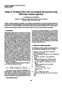
· It took another 20 iterations for the algorithm in phase 2 to converge. The denominator coefficients were found to be d11 = –1.5230137262, d12 = 0.9500000026. The coefficients of numerator a(z) are shown in the figure below. Coeffients of Numerator a(z) 0.07 0.06 0.05 0.04 0.03 0.02 0.01 0 −0.01 −0.02 −0.03
0
5
10
15
20
13
25
30
35
· maximum passband ripple: 0.0325 · minimum stopband attenuation: 29.7270 dB · passband group delay 21 with maximum ripple 0.1818 · magnitude of the two poles: 0.9747 · number of zeros in numerator: 16 ======== Comparison 1 ======= · Compare with an equivalent nonsparse IIR filter of order (n = 19, r = 1) with the same design specifications: · maximum passband ripple: 0.0676 · minimum stopband attenuation: 23.4019 dB · passband group delay 12 with maximum ripple 0.4579 14
Amplitude responses 5 0 −5 −10 −15 −20 −25 −30 −35 −40 −45
0
0.1
0.2
0.3
0.4 0.5 0.6 Normalized frequency 15
0.7
0.8
0.9
1
======== Comparison 2 ======= · Compared with an equiripple linear-phase FIR filter of order of length 88 that was designed using the ParksMcClellan algorithm with the same design specifications · and comparable maximum passband ripple and · comparable minimum stopband attenuation · passband group delay = 43.5 (versus 21) · 44 multiplications versus 18 multiplications per output sample required by the sparse IIR filter.
16
5. Concluding Remarks • The proposed technique works for minimax design of stable
IIR
filters
with
sparse
coefficients.
The
performance of these filters appears to be satisfactory compared with their non-sparse counterparts. • A drawback of these filters is the longer group delay relative to their non-sparse counterparts, thus a topic of future research: sparse filters with low group delay. • Implementation irregularly
techniques
located
zero
investigation.
17
for
sparse
coefficients
filters
seems
with worth