of the numerator as a semi-definite programming problem. Therefore, linear and convex quadratic inequalities such as peak error constraints and prescribed ...
DESIGN OF CONSTRAINED IIR AND INTERPOLATED IIR FILTERS USING A NEW SEMI-DEFINITE PROGRAMMING BASED MODEL REDUCTION TECHNIQUE S. C. Chan, K. M. Tsui and K. W. Tse Department of Electrical and Electronic Engineering, The University of Hong Kong, Pokfulam Road, Hong Kong.
ABSTRACT This paper proposes a new method for designing IIR filter with peak error constraints and prescribed flatness constraints, such as zeros at stopband. It is based on the model reduction of a FIR function that satisfies the specification by extending a method previously proposed by Brandenstein et al. The proposed model reduction method retains the denominator of the conventional techniques and formulates the optimal design of the numerator as a semi-definite programming problem. Therefore, linear and convex quadratic inequalities such as peak error constraints and prescribed number of zeros at the stopband for the IIR filters can be imposed and solved optimally. Moreover, a method is also proposed to facilitate the efficient implementation of the model reduced IIR filters in multirate applications. Design examples show that the proposed method gives better performance, and more flexibility in incorporating a wide variety of constraints than conventional methods.
I. INTRODUCTION The design of approximately linear-phase IIR filters is traditionally being considered as a very difficult problem, because the performance measure such as the least squares or minimax errors and the stability constraint are highly nonlinear functions of the filter coefficients. It usually involves constrained nonlinear optimization, whose performance is rather sensitive to the initial guess. Very often, the optimization software will converge to unsatisfactory local minimum if the initial guess is inappropriately chosen. Another indirect but useful method for designing IIR filters is based on model reduction [1,2] of FIR prototype filters, which can be designed easily and optimally using existing methods such the Remez exchange algorithm and semi- definite or infinite programming. Basically, a FIR prototype filter with the given specifications is first designed. Model reduction is then applied to convert this FIR filter to an IIR filter of reduced order, having a similar characteristic as the original FIR filters. In addition to its simple design procedure, the advantage of the model reduction approach is that the resulting IIR filter is guaranteed to be stable, and the frequency characteristics such as the phase response of the FIR prototype filter is well preserved. However, it does not allow precise control of the frequency response and other constraints, such as prescribed number of zeros at the stopband or peak ripple constraints, to be imposed. One would also expect the performance of the model-reduced filter to be sub-optimal and it can be further improved. In this paper, we propose a new design method for IIR filters using a new constrained model reduction technique, which is a modification of the model reduction method proposed in [2]. Important advantages of the method in [2] are that the numerator and denominator can be determined separately and the stability of the model-reduced filter is guaranteed. More precisely, the denominator is first determined, followed by the numerator. This property allows us to incorporate linear and convex quadratic constraints and shape the frequency response of the final IIR filter by designing the numerator using semi-definite programming (SDP), given the denominator at the first stage. For illustrative purpose, we mainly focus on the incorporation of peak stopband error and prescribed number of zeros at the stopband to the final IIR filters. The former is useful to limit the undesirable sidelobes at the band edges and design results show that it yields
141
considerable better performance compared to conventional model reduction methods. It should be noted that given the denominator, the design of the numerator using SDP with linear and convex quadratic inequalities is a convex optimization problem. In other words, the solution, given the denominator, is guaranteed to be optimal. Owing to the improved frequency characteristics of the proposed design method, further optimization is usually not required. Since the constraints for prescribed number of zeros are just linear equality constraint after the denominator has been determined, they can be incorporated easily under the SDP framework. Interested readers are referred to [3] for more details of SDP in filter design. Moreover, we also proposed a modification of the new model reduction method so that the denominator of the modelreduced filter is of the form Q(zM), where M is an integer. This is very useful in expressing the model-reduced filters in its polyphase representation, which provides efficient implementation of decimation/interpolation filters and other multirate applications [4]. Using these results, the design approach is further extended to the design of interpolated IIR filters, which exhibit comparable implementation complexity and performance but a lower system delay than conventional linear-phase interpolated FIR (IFIR) filters [5]. The paper is organized as follows: The model reduction technique proposed in [2] and the principle of the proposed constrained model reduction are described in Section II. The details of the SDP formulation of the peak design error and magnitude flatness constraints for the IIR filters are given in section III. The method to express the denominator of the model-reduced filter as Q(zM) is also proposed. Design examples, including the design of interpolated IIR filter, are given in Section IV to demonstrate the effectiveness of the proposed approach. Finally, conclusion is drawn in Section V.
II. MODEL REDUCTION To start with, suppose that we have designed the FIR filter H ( z ) = ∑nL=−10 h(n) z − n using any existing methods in the literature, the model reduction technique proposed in [2] is then applied to convert H (z ) to an IIR filter Hˆ ( z ) with the following form: P ( z ) ∑nL=p0−1 p (n) z − n Hˆ ( z ) = , q ( 0) = 1 , L p ≥ Lq , = (2-1) Q( z ) ∑nL=q0−1 q (n) z − n where L p and Lq are respectively the length of numerator and denominator of Hˆ ( z ) . As mentioned earlier, the advantage of this method is that P(z) and Q(z) can be determined separately. More precisely, Q(z) can be found without the knowledge of P(z). Therefore, unlike other model reduction technique, additional constraints can be readily incorporated during the determination of P(z), after Q(z) is found. A. — Determination of denominator In [2], a simple iterative design procedure was proposed to determine Q(z). First of all, let’s consider the following polynomial, which approximates Q(z)in the k-th iteration: (2-2) Q ( k ) ( z ) = 1 + ∑nL=q 1−1 q ( k ) (n) z − n , Q ( 0) ( z ) = 1 . By defining: X ( k ) ( z ) = z − ( L −1) H ( z −1 ) / Q ( k −1) ( z ) = ∑∞n=0 x ( k ) (n) z − n , (2-3)
q ( k ) (n) can be calculated by minimizing the following objective function:
F ( k ) (q ( k ) ) = ( B ( k ) q ( k ) − d ( k ) ) T ⋅ ( B ( k ) q ( k ) − d ( k ) ) ,
B(k )
where
approximate H (z ) with small enough errors using the technique in [2], we found that the length of the denominator of Hˆ ( z ) should satisfy the following condition:
(2-4)
O 0 , x ( k ) (0) L M (k ) L x ( L − Lq )
x ( 0) 0 (k ) (k ) x x ( 1 ) ( 0) M M = (k ) (k ) x ( Lq − 2) x ( Lq − 3) M M (k ) x ( L − 2) x ( k ) ( L − 3) (k )
0 M
L O
Lq ≥ τ + 1 ,
q ( k ) = [q ( k ) ( Lq − 1),..., q ( k ) (1)]T and
d ( k ) = −[0,...,0, x ( k ) (0),..., x ( k ) ( L − Lq − 1)]T .
The basic idea is to find q (k ) such that F ( k ) (q ( k ) ) is the smallest among all the iterations for a sufficiently large k. More importantly, the roots of the resulting Q ( k ) ( z ) , which minimizes F ( k ) (q ( k ) ) for an arbitrarily given X ( k ) ( z ) , are proved to lie strictly inside the unit circle, and thus Hˆ ( z ) is always stable.
(2-9)
where w denotes the integer just larger than or equal to w. (29) tells us that the savings of number of multiplications and additions would be more significant if model reduction is applied to FIR functions with lower system delay. Here, we prefer to choose D such that: τ ≅ L/4 . (2-10) This approximation allows us to reduce the system delay of H ( z ) as much as possible, while keeping a good frequency characteristic of H ( z ) . It should be noted that a dump would appear at the transition band when the group delay is lower than that in (2-10). According to (2-10), the implementation complexity of Hˆ ( z ) would be comparable to its linear phase
Interested readers are referred to [2] for more details.
counterpart, which has similar frequency characteristic as that of Hˆ ( z ) . The system delay on the other hand is considerably
B. — Determination of numerator using SDP
lower.
Once Q(z ) is designed, we want to approximate the response of H (z ) by P (z ) , given Q(z ) , in the least square (LS) sense. That is: π
ELS ( p) = ∫−π | {P(e jω ) Q(e jω )} − H (e jω ) |2 dω ,
(2-5)
where p = [ p (0),..., p ( L p − 1)] . (2-5) can be written as the T
following matrix form: min p T Up + p T g + a ,
(2-6)
p
}
2
where
2
a = ∫−π H (e jω ) dω . This is a standard quadratic programming problem, which can be solved readily. However, large sidelodes are usually encountered at the band-edge of the model-reduced filter. Therefore, additional constraints on the stopband ripple constraints should be imposed to improve the frequency characteristic. Here, we formulate (2-6) as a SDP problem. To start with, one can decompose U as U = G T G so that it can be reformulated, by means of Schur complement [6], as the following linear matrix inequality (LMI): min c T x x
δ − p T g − a subject to Gp
pT G T f 0, 1
(2-7)
where c = [1,0,....0]T and x = [δ pT ]T .The advantage of formulating the objective function as LMI is that the resulting problem is convex and the optimal solution, if it exists, can be found. In addition, additional linear equalities and convex quadratic constraints can also be formulated as LMIs, as we shall illustrate in later sections. C. — Selection of the length of denominator Suppose that the desired passband response of H (z ) , denoted by H p (z ) , is given by: H p (e jω ) = e − jωτ , ω in the passband.
(3-1) (3-2)
γ R (ω ) = p ⋅ Re{e (ω )} , γ I (ω ) = p ⋅ Im{e (ω )} and T
where [g ]n = ∫−ππ Re H (e jω )Q(e jω ) ⋅ e jωn / Q(e jω ) dω and π
constraints are given by: | Hˆ (e jω ) |2 ≤ ε , ω in the stopband.
ε ≥ γ R2 (ω ) + γ I2 (ω ) ,
[U ]n1, n 2 = ∫−π e jω ( n 2 − n1) / Q (e jω ) dω ,
{
A. — Peak stopband error constraint Denote ε as the prescribed peak stopband ripple to be imposed on the model-reduced filter Hˆ ( z ) . These convex quadratic
Substituting (2-1) into (3-1), given Q( z ) , one gets:
2
π
III. DESIGN OF CONSTRAINED IIR FILTER
(2-8)
where τ = ( L − 1) / 2 − D is the passband group delay of H (z ) ; D is the prescribed delay reduction parameter ( D = 0 corresponds to its linear-phase counterpart). In order to
142
T
− j ( L −1)ω
e (ω ) = [1, e − jω ,..., e p ]T / Q(e jω ) . Using Schur complement [6], it can be shown that the constraints in (3-2) are equivalent to: γ R (ω ) γ I (ω ) ε 1 0 f 0. Λ ( p) = γ R (ω ) (3-3) γ I (ω ) 0 1 Digitizing (3-3), these constraints on the peak ripples can be augmented to the existing LMI in (2-7) for determining P( z ) . B. — Imposing linear equality constraint To impose U ω − 1 zeros on Hˆ ( z ) at ω = ω in the stopband, the following relation should be satisfied: du ˆ H (ω ) = 0 , u = 0,1,K,U ω − 1 . (3-4) dz u ω =ω (3-4) is equivalent to: du P(ω ) = 0 , u = 0,1,K,U ω − 1 . dz u ω =ω
(3-5)
Expanding (3-5) and after slight manipulation, one gets a set of linear equality constraints as follows: L −1 u − jω n (3-6) ∑ n =p 0 n e p(n) = 0 , u = 0,1,K,U ω − 1 , and its matrix form is given by: A⋅ p = b , (3-7) where [ A]u , n = nu e − jω n and [b]u = 0 . Here, [ A]m,n denotes the (m, n) − th entry of a ( U ω × L p ) matrix A . Assume that the number of constraints is smaller than the number of variables, part of the variables, called the redundant variables, can be expressed in terms of the remaining variables, called the
independent variables, when solving the SDP. First of all, rewrite (3-7) as follows: p AL p − r Ar ⋅ L p − r = b , (3-8) pr
[
]
where A = [ AL p − r
Ar ] ; p = [ p LT p − r
prT ]T ; and r is the
number of redundant variables in P ( z ) . Using (3-19), p can be written in terms of p L p − r as: O I L p − r p = L−p1− r + pL p −r , −1 Ar b − Ar AL p − r
(3-9)
where I N is an ( N × N ) identity matrix; O N is an N column zero vector. By substituting (3-9) into (2-7), hL p −r can be found optimally by SDP, while satisfying the prescribed constraints. C. — Polyphase decomposition Polyphase representation of digital filters is useful to the efficient implementation of decimation/interpolation filters, as well as other multirate systems [4]. However, expressing the IIR filters in the form of (2-1) is rather inefficient. To do so, one should factorize the denominator Q( z ) as follows [7]:
Q( z ) = ∏kLq=1−1 (1 − λk z −1 ) ,
(3-10)
where λk is the roots of Q( z ) . Using the following identity: (1 − λk z −1 ) ≡ (1 − λMk z − M ) / ∑mM=−01λmk z − m ,
(3-11)
where M is an integer, (3-11) can be written as follows: ~ (∑ L p −1 p (n) z − n )(∏kLq=1−1 (∑mM=−01λmk z − m )) P ( z) Hˆ ( z ) = n =0 = ~ M , (3-12) Lq −1 M −M Q( z ) ∏k =1 (1 − λk z ) ~ ~ It is noticed that the length of P ( z ) and Q ( z ) increases considerably to M ( Lq − 1) − Lq + L p + 1 and M ( Lq − 1) + 1 , respectively. The M-th polyphase decomposition of (3-12) is: (3-13) Hˆ ( z ) = ∑mM=−01 z − m E m ( z M ) , ~ where E m ( z ) = E P~ ,m ( z ) / Q ( z ) is the m-th polyphase component ~ of Hˆ ( z ) ; E P~ ,m ( z ) is the m-th polyphase component of P ( z ) .
The drawback of this approach is that the numerical error of estimating the roots of Q(z ) would be large when Lq is large. ~ ~ Moreover, the length of P ( z ) and Q ( z ) is unnecessarily long when M is large. Since what is required is a denominator polynominal in z M , it is desirable to generate such a representation directly from model reduction. To this end, the design procedure of determining the denominator, as described in section II-A, is modified. Instead of using the rational function as in (2-1), the model-reduced filter is assumed to have the following form: L −1 −n P( z ) ∑ p p(n) z , q(0) = 1 , L ≥ dM + 1 Hˆ ( z ) = = nd=0 (3-14) p − nM M Q ( z ) ∑n = 0 q ( n) z
where d corresponds to the number of non-zero coefficients of Q ( z M ) , excluding q(0) . The vector q ( k ) in (2-4) is modified as follows: q ( k ) = [ q ( k ) ( dM ), q ( k ) ((d − 1) M ),..., q ( k ) ( M )]T , (3-15) which can be solved by considering the corresponding rows of B ( k ) and d ( k ) . According to [2], this modification does not violate the stability theorem, which holds for arbitrarily given X ( k ) ( z ) . Hence, the model-reduced filter in the form of (3-14) is still stable, provided that F ( k ) (q ( k ) ) is the smallest. More importantly, design result shows that the length of numerator and denominator is less than that using the direct expansion as described previously.
143
IV. DESIGN EXAMPLES Example 1: Low-delay IIR lowpass filters In this example, low-delay IIR lowpass filters are designed using the proposed constrained model reduction. The passband and stopband cutoff frequencies are respectively ω p = 0.45π
and ω s = 0.55π . A low-delay FIR prototype filter of length L = 45 and delay reduction parameter D = 11 is first designed using SDP [8] so that its passband group delay is about 11 samples. Model reduction is then applied to convert this prototype filter to an IIR filter. According to section II-C, it is sufficient to choose the length of numerator and denominator of the modelreduced filter as L p = 13 and Lq = 13 , respectively. Model reducing this prototype filter without any constraints gives a passband error of 0.063 dB and a stopband error of 36.74 dB, as shown by the solid line in figure 1a and 1b. To limit the sidelobe at the band edge, peak stopband error constraint of 40 dB is imposed to the model-reduced filter. In addition, one zero at ω = π is also imposed. Figure 1 shows the design results of the IIR filter so obtained. It can be seen from the dash-dotted line in figure 1a and 1b that the maximum stopband attenuation of the proposed IIR filter is now increased to 40dB at the expense of slightly lower performance at the passband. Also, as depicted in figure 1d, the proposed IIR filter has one zero at ω = π . In view of the implementation complexity, the proposed IIR filter requires 25 multipliers and 23 adders, which are about half of those required for this low-delay prototype FIR filter, and are comparable to those of linear-phase FIR filter of length 41. To express the above IIR filter in its polyphase representation with M = 4, the length of the numerator and denominator of the above IIR filter becomes 49 using the identity in (3-11). Therefore, the total number of nonzero coefficients is 62. To illustrate the flexibility of our approach, the denominator is constrained to the form Q ( z 4 ) . The number of non-zero coefficients and length of the denominator are 7 and 25, respectively (i.e. d = 6), and the length of the numerator is chosen to be 25. Its number of non-zero coefficients is only 32. Employing the proposed model reduction without any constraints, the corresponding passband deviation and stopband attenuation are 0.064 dB and 38.38 dB, respectively. Again, additional constraints, including peak stopband error constraint of 40 dB and two zeros at ω = π , are imposed to shape the frequency response of the model-reduced filter. Figure 2 shows the frequency and impulse response of the IIR filter so obtained. As seen from figure 2, all constraints are satisfied. Example 2: Low-delay interpolated IIR (I-IIR) filter Interpolated FIR (IFIR) filters [8] are useful FIR filter structure with significant savings in arithmetic complexities compared to the traditional direct form FIR filters. The basic idea is to implement the FIR filter in the form F ( z ) = G ( z M ) I ( z ) , i.e. a cascade of two FIR filters, where the model filter G(z) is used to meet the narrow transition band of the desired specification and I (z ) is used to eliminate the extra images that are created by G ( z M ) . In general, IFIR filters are applicable to both linearphase and low-delay case. Here, we consider the application of model reduction to the low-delay IFIR filter so that both the system delay and implementation complexity of the resulting filter, which we call the interpolated IIR (I-IIR) filter, can be further reduced. As an illustration, we shall consider the design of a narrowband lowpass filter with the following specifications: ω p = 0.09π , ω s = 0.11π , δ p = 0.02 (0.172 dB), δ s = 0.01 (40
dB) and M = 5 . To meet the above specifications, the lowdelay model filter G(z) has a length of 45 and passband group delay of 11 samples. While for the image suppressor I (z ) , its length and passband group delay are 25 and 6 respectively. As
discussed in section II-C, the lengths of both numerator and denominator of Gˆ ( z ) and Iˆ( z ) are chosen to be respectively 12 and 7. The proposed model reduction with 40 dB peak stopband constraints is then applied to both low-delay FIR filters. Figure 3 (dash-dotted line) shows the frequency and group delay responses of the I-IIR filter so obtained. The passband deviation is 0.117 dB and the stopband attenuation is 40 dB. For comparison purpose, a FIR counterpart of the above I-IIR filter are designed, where G (z ) and I (z ) are linear-phase FIR lowpass filters with lengths 41 and 19, respectively. Its frequency and group delay responses are also plotted as solid line in figure 3a and 3b, respectively. The corresponding passband deviation and stopband attenuation are respectively 0.169 dB and 40 dB, which are comparable to our design. However, this linear-phase IFIR filter has a passband group delay of 109 samples, which is significantly higher than that of the I-IIR filter (about 61 samples). Regarding the implementation complexity, the proposed I-IIR requires 36 multipliers and 34 adders, while the linear-phase IFIR filter requires 30 multipliers and 28 adders. According to the discussion in section III-C, one can express the I-IIR filter in the polyphase representation with reduced implementation complexity compared to the direct expansion of denominator as described from (3-10) to (3-13). However, details are omitted due to page limitation. In summary, one can do so by assuming the model-reduced filter of I (z ) with the following form: (4-1) Iˆ( z ) = P ( z ) / Q ( z M ) . I
[4]
P. P. Vaidyanathan, “Multirate Systems and Filter Banks,” Englewood Cliffs, NJ: Prentice Hall, 1993. [5] Y. Neuvo, D. Cheng-Yu and S. K. Mitra, “Interpolated finite impulse response filters,” IEEE Trans. ASSP, vol. 32, pp. 563-570, June 1984. [6] H. Wolkowicz, R. Saigal and L. Vandenberge, “Handbook of Semidefinite Programming: theory, algorithms, and applications”, Kluwer Academic Publishers, 2000. [7] M. G. Bellanger, G. Bonnerot and M. Coudreuse, “Digital Filtering by Polyphase Network: Application to Sample-rate Alteration and Filter Banks,” IEEE Trans. ASSP, vol. 24, no. 2, pp. 109-114, April 1976. [8] W.-S Lu, “Design of nonlinear-phase FIR digital filters: A semidefinite programming approach”, ISCAS’99, vol. III, pp. 263266, Orlando, FL, May 1999. [9] T. Saramaki, Y. Neuvo and S. K. Mitra, “Design of computationally efficient interpolated FIR filters,” IEEE Trans. Circuits Syst., vol. 35, pp. 70-88, Jan. 1988. [10] Y. C. Lim, “Frequency response masking approach for the synthesis of sharp linear phase digital filters,” IEEE Trans. Circuits Syst., vol. 33, pp. 357-364, April 1986.
1a)
1b)
I
Consequently, the m-th polyphase component of the resulting IIIR is given by: PG ( z ) E PI ,m ( z ) , m = 0,1,K, M − 1 , E F ,m ( z ) = (4-2) QG ( z )QI ( z ) where PG (z ) and QG (z ) are the numerator and denominator of the model-reduced filter of G (z ) ; E PI ,m ( z ) is the m-th 1c) 1d) Figure 1. Design results of low-delay IIR filters in example 1 (peak stopband error constraint ε = 40 dB and one zero at ω = π). a) – c) Frequency response (passband details in smaller figure), stopband details and group delay response of lowpass IIR filters: dash-dotted line – proposed IIR filter; solid line – modelreduced FIR filter. d) Pole-zero plot of proposed IIR filter.
polyphase component of PI (z ) . Finally, the proposed design technique can also be applied to the more generalized IFIR approach [9] and frequency response masking approach [10]. It is expected that the resulting filters will achieve lower implementation complexity in the low-delay case.
V. CONCLUSION A new method for designing IIR filters with peak error and magnitude flatness constraints is proposed. It is based on the model reduction of FIR prototype filters by a new model reduction technique. The proposed model reduction method retains the denominator of the conventional techniques and formulates the optimal design of the numerator as a semidefinite programming problem. Linear and convex quadratic inequalities such as peak error constraints and prescribed number of zeros at the stopband for the IIR filters can be imposed and solved optimally. Moreover, a method to express the denominator of the model-reduced filter in terms of the integer power of z is also proposed. Design examples show that the proposed method gives better performance and more flexibility in incorporating a wide variety of constraints than conventional methods.
2a) 2b) Figure 2: Design results of low-delay IIR filters, in which the denominator is the polynomial in z4, in example 1 (peak stopband error constraint ε = 40 dB and two zeros at ω = π). a) Frequency response. b) Impulse response of the numerator (top) and denominator (bottom).
REFERENCES [1] [2] [3]
B. C. Moore, “Principal component analysis in linear system: Controllability, observability, and model reduction,” IEEE Trans. Automat. Contr., vol. AC-26, pp. 17-31, 1981. H. Brandenstein and R. Unbehauen, “Least-squares approximation of FIR by IIR filters,” IEEE Trans. Signal Processing, vol. 46, no. 1, pp. 21-30, Jan 1998. W.-S Lu and A. Antoniou, “Design of Digital Filters and Filter Banks by Optimization: A state of the Art Review,” in Proc. EUSIPCO’2000, vol. 1, pp. 351-354, Sep. 2000.
3a) 3b) Figure 3. Design results of low-delay interpolated IIR filter in example 2 (peak stopband error constraint ε = 40 dB for both G(z) and I(z)): a) and b) Frequency response (passband details in smaller figure) and group delay response of narrowband lowpass filters: dash-dotted line – proposed I-IIR filter; solid line – linear-phase IFIR filter.
144