Minimax Pointwise Redundancy for Memoryless Models over Large Alphabets Wojciech Szpankowski, Marcelo J. Weinberger HP Laboratories HPL-2012-87 Keyword(s): data compression; redundancy; large alphabets; generating functions; saddle point method.
Abstract: We study the minimax pointwise redundancy of universal coding for memoryless models over large alphabets and present two main results: We first complete studies initiated in Orlitsky and Santhanam deriving precise asymptotics of the minimax pointwise redundancy for all ranges of the alphabet size relative to the sequence length. Second, we consider the minimax pointwise redundancy for a family of models in which some symbol probabilities are fixed. The latter problem leads to a binomial sum for functions with super-polynomial growth. Our findings can be used to approximate numerically the minimax pointwise redundancy for various ranges of the sequence length and the alphabet size. These results are obtained by analytic techniques such as tree-like generating functions and the saddle point method.
External Posting Date: April 23, 2012 [Fulltext] Internal Posting Date: April 23, 2012 [Fulltext]
Approved for External Publication
Copyright 2012 Hewlett-Packard Development Company, L.P.
Minimax Pointwise Redundancy for Memoryless Models over Large Alphabets∗ Wojciech Szpankowski† Department of Computer Science, Purdue University W. Lafayette, IN 47907, U.S.A.,
[email protected] Marcelo J. Weinberger Hewlett-Packard Laboratories Palo Alto, CA 94304, U.S.A.,
[email protected]
Abstract—We study the minimax pointwise redundancy of universal coding for memoryless models over large alphabets and present two main results: We first complete studies initiated in Orlitsky and Santhanam [15] deriving precise asymptotics of the minimax pointwise redundancy for all ranges of the alphabet size relative to the sequence length. Second, we consider the minimax pointwise redundancy for a family of models in which some symbol probabilities are fixed. The latter problem leads to a binomial sum for functions with super-polynomial growth. Our findings can be used to approximate numerically the minimax pointwise redundancy for various ranges of the sequence length and the alphabet size. These results are obtained by analytic techniques such as tree-like generating functions and the saddle point method.
I. I NTRODUCTION The classical universal source coding problem [4] is typically concerned with a known source alphabet whose size is much smaller than the sequence length. In this setting, the asymptotic analysis of universal schemes assumes a regime in which the alphabet size remains fixed as the sequence length grows. More recently, the case in which the alphabet size is very large, often comparable to the length of the source sequences, has been studied from two different perspectives. In one setup (motivated by applications such as text compression over an alphabet composed of words), the alphabet is assumed unknown or even infinite (see, e.g., [2], [9], [12], [16], [18]). In another setup (see, e.g., [15]), the alphabet is still known ∗
The material in this paper was presented in part at the 2010 IEEE International Symposium on Information Theory, Austin, Texas, USA, June 2010. † This author’s contribution was partially made when visiting Hewlett–Packard Laboratories, Palo Alto, CA 94304, U.S.A. This author was also supported by the NSF STC Grant CCF-0939370, NSF Grants DMS-0800568 and CCF-0830140, AFOSR Grant FA865511-1-3076, NSA Grant H98230-08-1-0092, and MNSW grant N206 369739.
and finite (as in applications such as speech and image coding), but the asymptotic regime is such that both the size of the alphabet and the length of the source sequence are very large. Notice that, in this scenario, the optimality criteria and the corresponding optimal codes do not differ from the classical approach; rather, it is the asymptotic analysis that is affected. In this paper, we follow the latter scenario, targeting a classical figure of merit: the minimax (worstcase) pointwise redundancy (regret) [19]. Specifically, we derive precise asymptotic results for two memoryless model families. To recall, the pointwise redundancy of a code arises in a deterministic setting involving individual data sequences, where probability distributions are mere tools for describing a choice of coding strategies. In this framework, given an individual sequence, the pointwise redundancy of a code is measured with respect to a (probabilistic) model family (i.e., a collection of probability distributions that reflects limited knowledge about the data-generating mechanism). The pointwise redundancy determines by how much the code length exceeds that of the code corresponding to the best model in the family (see, e.g., [14] and [23] for an in-depth discussion of this framework). In the minimax pointwise scenario, one designs the best code for the worst-case sequence, as discussed next. A fixed-to-variable code Cn : An → {0, 1}∗ is an injective mapping from the set An of all sequences of length n over the finite alphabet A of size m = |A| to the set {0, 1}∗ of all binary sequences. We assume that Cn satisfies the prefix condition and denote L(Cn , xn1 ) the code length it assigns to a sequence xn1 = x1 , . . . , xn ∈ An . A prefix code matched to a model P (given by a probability distribution P over An ) encodes xn1 with an “ideal” code length − log P (xn1 ), where log := log2 will denote the binary logarithm throughout the paper, and we ignore the integer length constraint. Given a sequence
2
xn1 , the pointwise redundancy of Cn with respect to a model family S (such as the family of memoryless models M0 ) is thus given by Rn (Cn , xn1 ; S) = L(Cn , xn1 ) + sup log P (xn1 ). P ∈S
Finally, the minimax pointwise redundancy Rn∗ (S) for the family S is given by Rn∗ (S) = min max Rn (Cn , xn1 ; S) . n Cn
x1
(1)
This quantity was studied by Shtarkov [19], who found that, ignoring the integer length constraint also for Cn (cf. [5]),
Rn∗ (S) = log
∑ x
n 1
sup P (xn1 )
P ∈S
(2)
and is achieved with a code that assigns to each sequence a code length proportional to its maximum-likelihood probability over S . In particular, for S = M0 , precise asymptotics of Rn∗ (M0 ) have been derived in the regime in which the alphabet size m is treated as a constant [20] (cf. also [23]). The minimax pointwise redundancy was also studied when both n and m are large, by Orlitsky and Santhanam [15]. Formulating this scenario as a sequence of problems in which m varies with n, leading term asymptotics for m = o(n) and n = o(m), as well as bounds for m = Θ(n), are established in [15].1 The goal of this formulation is to estimate Rn∗ (M0 ) for given values of n and m, which fall in one of the above cases. In this paper we first provide, in Theorem 1, precise asymptotics of Rn∗ (M0 ) for all ranges of m relative to n. Our findings are obtained by analytic methods of analysis of algorithms [8], [21]. Theorem 1 not only completes the study of [15] by covering all ranges of m (including m = Θ(n)), but also strengthens it by providing more precise asymptotics. Indeed, it will be shown that the error incurred by neglecting lower order terms may actually be quite significant, to the point that, for m = o(n), the first two terms of the asymptotic expansion for constant m given in [20] is a better approximation to Rn∗ (M0 ) than the leading term established in [15]. In addition, Theorem 1 also enables a precise analysis of the minimax pointwise redundancy in a more general scenario. Specifically, we consider the alphabet A ∪ B , with |A| = m and |B| = M , and a (memoryless) f0 , in which the probabilities model family, denoted M 1 We write f (n) = O(g(n)) if and only if |f (n)| ≤ C|g(n)| for some positive constant C and sufficiently large n. Also, f (n) = Θ(g(n)) if and only if f (n) = O(g(n)) and g(n) = O(f (n)), f (n) = o(g(n)) if and only if limn→∞ f (n)/g(n) = 0, and f (n) = Ω(g(n)) if and only if g(n) = O(f (n)).
of symbols in B are fixed, while m may be large.2 Such constrained model families, which correspond to partial knowledge of the data-generating mechanism, fill the gap between two classical paradigms: one in which a code is designed for a specific distribution in M0 (Shannontype coding), and universal coding in M0 . For example, consider a situation in which data sequences from two different sources (over disjoint alphabets) are randomly interleaved (e.g., by a router), as proposed in [1], and assume that one of the sequences is (controlled) simulation data, for which the generating mechanism is known. If we further assume that the switching probabilities are also known, this situation falls under the proposed setting, where B corresponds to the alphabet of the simulation data. Other constrained model families have been studied in the literature as means to reduce the number of free parameters in the probability model (see [22] for an example motivated in image coding). Given our knowledge of the distribution on B, one would expect to “pay” a smaller price for universality in terms of redundancy. In a probabilistic setting and for m treated as a constant, Rissanen’s lower bound on the (average) redundancy [17] is indeed proportional to the number m − 1 of free parameters. Moreover, it is easy to see that the leading term asymptotics of the pointwise redundancy of a (sequential) code that uses a fixed probability assignment for symbols in B , and one based on the Krichevskii-Trofimov scheme [13] for symbols in A, are indeed the same as those for Rn∗ (M0 ). However, this intuition notwithstanding, notice that the minimax scheme for the combined alphabet does not encode the two alphabets separately. Moreover, the analysis is more complex for unbounded m, especially when we are interested in more precise asymptotics. In this paper, we formalize the above intuition by providing precise asymptotics of the minimax pointwise f0 ), again for all ranges of m (relative redundancy Rn∗ (M to n). We first prove that f0 ) Rn∗ (M
= log
n ∑ k=0
( )
n k ∗ p (1 − p)n−k 2Rk (M0 ) k
(3)
where p = 1−P (B). As it turns out, in order to estimate this quantity asymptotically, we need a quite precise understanding of the asymptotic behavior of Rk∗ (M0 ) for large k and m, as provided by Theorem 1. The study of the minimax pointwise redundancy over A ∪ B expressed in (3) leads to an interesting problem f0 are defined over Note that the model families M0 and M f different alphabets. In addition, the family M0 is constrained in that the probabilities of symbols in B take fixed values. 2
3
for the so called binomial sums, defined in general as ( )
Sf (n) =
∑ n
k
k
pk (1 − p)n−k f (k)
(4)
where 0 < p < 1 is a fixed probability and f is a given function. In [6], [11], asymptotics of Sf (n) were derived for the polynomially growing function f (x) = O(xa ). This result applies to our case when m is a constant, and f0 ) leads to the conclusion that the asymptotics of Rn∗ (M ∗ are the same as those of Rnp (M0 ), an intuitively appealing result since the length of the sub-sequence over A is np with high probability. But when m also grows, we encounter sub-exponential, exponential and super-exponential functions f , depending on the relation between m and n; therefore, we need more precise information about f to extract precise asymptotics of Sf (n). In our second main result, Theorem 2, we use the asymptotics derived in Theorem 1 to deal with the f0 ) binomial sum (3) and extract asymptotics of Rn∗ (M for large n and m. In the remainder of this paper, Section II reviews the analytic methods of analysis of algorithms that were used in [20] for estimating Rn∗ (M0 ) in the constant m case, as well as the saddle point method, whereas Section III presents our main results. These results are proved in Section IV. II. BACKGROUND In the sequel, we will denote dn,m := Rn∗ (M0 ) to emphasize the dependence of Rn∗ (M0 ) on both n and m. We will also denote dn,m := log Dn,m which, by (2), implies ∑ Dn,m = sup P (xn1 ) . (5) P ∈M0 xn 1
Clearly, Dn,m takes the form Dn,m =
∑ k1 +···+km =n
(
n k1 , . . . , km
)(
k1 n
)k1
(
km ··· n
)km
(6) where ki is the number of times symbol i ∈ A occurs in a string of length n. The asymptotics of the sequence of numbers ⟨Dn,m ⟩, (for m constant), are analyzed in [20] through its socalled tree-like generating function, defined as Dm (z) =
∞ ∑ n=0
nn n!
Dn,m z n .
Here, we will follow the same methodology, which we review next. The first step is to use (6) to define an appropriate recurrence on ⟨Dn,m ⟩ (involving both indexes, n and m), and to employ the convolution formula for
generating functions (cf. [21]) to relate Dm (z) to the tree-like generating function of the sequence ⟨1, 1, . . .⟩, namely ∞ ∑ kk k z . B(z) = k! k=0 This function, in turn, can be shown to satisfy (cf. [21]) 1 B(z) = (7) 1 − T (z) for |z| < e−1 , where T (z) is the well-known tree function, which is a solution to the implicit equation T (z) = zeT (z)
(8)
with |T (z)| < 1.3 Specifically, the following relation is proved in [20]. Lemma 1: The tree-like generating function Dm (z) of ⟨Dn,m ⟩ satisfies, for |z| < e−1 , Dm (z) = [B(z)]m − 1
and, consequently, n! n [z ] [B(z)]m (9) nn where [z n ]f (z) denotes the coefficient of z n in f (z). Defining β(z) = B(z/e), |z| < 1, noticing that n [z ]β(z) = e−n [z n ]B(z), and applying Stirling’s formula, (9) yields ( ) √ Dn,m = 2πn 1 + O(n−1 ) [z n ] [β(z)]m . (10) Dn,m =
Thus, it suffices to extract asymptotics of the coefficient at z n of [β(z)]m , for which a standard tool is Cauchy’s coefficient formula [8], [21], that is, I m 1 β (z) [z n ][β(z)]m = dz (11) 2πi z n+1 where the integration is around a closed path containing z = 0 inside which β m (z) is analytic. Now, the constant m case is solved in [20] by use of the Flajolet and Odlyzko singularity analysis [8], [21], which applies because [β(z)]m has algebraic singularities. Indeed, using (7) and (8), the singular expansion of β(z) around its singularity z = 1 takes the form [3] √ √ 1 1 2 β(z) = √ + − (1 − z) + O(1 − z). 24 2(1 − z) 3 The singularity analysis then yields [20]
( √
( )
dn,m =
n m−1 log 2 2
+ log
π
)
Γ( m 2)
√ ( ) Γ( m 1 2 )m log e √ 2 · +O (12) + m 1 n n 3Γ( 2 − 2 )
3 In terms of the standard Lambert-W function, we have T (z) = −W (−z).
4
for large n and constant m, where Γ is the Euler gamma function.4 When m also grows, which is the case of interest in this paper, the singularity analysis does not apply. Instead, the growth of the factor β m (z) determines that the saddle point method [8], [21], which we briefly review next, can be applied to (11). We will restrict our attention to a special case of the method, where the goal is to obtain an asymptotic approximation of the coefficient an := [z n ]g(z) for some analytic function g(z), namely I
I
1 g(z) 1 an = dz = eh(z) dz n+1 2πi z 2πi where h(z) := ln g(z) − (n + 1) ln z , under the assumption that h′ (z) has a real root z0 . The saddle point method is based on Taylor’s expansion of h(z) around z0 which, recalling that h′ (z0 ) = 0, yields 1 h(z) = h(z0 ) + (z − z0 )2 h′′ (z0 ) + O(h′′′ (z0 )(z − z0 )3 ). 2 (13) After choosing a path of integration that goes through z0 , and under certain assumptions on the function h(z), it can be shown (cf., e.g., [21]) that the first term of (13) gives a factor eh(z0 ) in an , the second term – after √ integrating a Gaussian integral – leads to a factor 1/ 2π|h′′ (z0 )|, and finally the third term determines the error term in the expansion of an . The standard saddle point method described in [21, Table 8.4] then yields the following lemma. Lemma 2: Assume the conditions required in [21, Table 8.4] hold and let z0 denote a real root of h′ (z). Then, (
(
eh(z0 ) h′′′ (z0 ) an = √ × 1 + O (h′′ (z0 ))ρ 2π|h′′ (z0 )|
case ρ = 3/2. The modified lemma will be the main tool in our derivation. III. M AIN R ESULTS In this section we present and discuss our main results, deferring their proof to Section IV. A. Model family M0 Theorem 1: For the memoryless model family M0 over an m-ary alphabet, where m → ∞ as n grows, the minimax pointwise redundancy dn,m behaves asymptotically as follows: (i) For m = o(n) √
dn,m =
m−1 n m m log e m log + log e + 2 m 2 ( 3 ) n √ 2 1 log e m m 1 − − +O +√ . (15) 2 4 n n m
(ii) For m = αn + ℓ(n), where α is a positive constant and ℓ(n) = o(n), dn,m = n log Bα + ℓ(n) log Cα − log (
where Cα :=
1 1 + 2 2
Aα := Cα +
and
dn,m
√
1+
4 α
2 α
)
(17) (18)
Bα := αCαα+2 e− Cα . 1
(14) (iii) For n = o(m)
4 As mentioned, Equation (2) ignores the integer length constraint of a code, and therefore O(1) terms in (12) are arguably irrelevant. This issue is addressed in [5]; here, we focus on the probability assignment problem, which unlike coding does not entail an integer length constraint. 5 This expression for the error term in (14) is obtained with the choice δ(n) = h′′ (z0 )−ρ/3 in [21, Table 8.4], provided certain conditions on h(z) are satisfied.
Aα
ℓ(n)2 log e ℓ(n)3 ℓ(n) 1 − + O +√ + 2nα2 Aα n2 n n (16)
))
for any constant ρ < 3/2, provided the error term is o(1).5 In order to control the error term, the conditions stated in [21, Table 8.4] include the requirement that, as n grows, h′′ (z0 ) → ∞. It turns out, however, that more is known for our particular h(z): indeed, it will be further shown that the growth of h′′ (z0 ) is at least linear. This additional property allows us to extend Lemma 2 to the
√
(19) (
)
1 n3 m 3 n(n−1) = n log + log e+O √ + 2 . n 2 m n m (20)
Discussion of Theorem 1 Significance and related work. The formulation of the scenario in which both n and m are large, as a sequence of problems where m varies with n, follows Orlitsky and Santhanam [15]. In a typical application of Theorem 1, for a given pair of values n = n0 and m = m0 , which are deemed to fall in one of the three itemized cases, the formulas are used to approximate the minimax pointwise redundancy dn0 ,m0 . The leading terms of the asymptotic expansions for m = o(n) and n = o(m) (i.e., (15) and (20)) were derived in [15].
5
Fig. 1. Value of the constant log Bα in the Θ(n) term of dn,m in case m = Θ(n).
The asymptotic expansion in (15) reveals that the error incurred by neglecting lower order terms may be significant. Consider the example in which n = 104 and m = 40 (or, approximately, m = n0.4 ). Then, the leading term in (15) is only 5.5 times larger than the second term, and 131 times larger than the third term. The error from neglecting these two terms is thus 15.4% (assuming all other terms are negligible). Even for n = 108 (and m = 1600), the error is still over 8%. It is interesting to notice that (15) is a “direct scaling” of (12): using Stirling’s approximation to replace Γ(x) in (12) by its √ asymptotic value 2π/x(x/e)x , and further approxi√ mating (1 + 1/x)(x+1)/2 with e (1 + 1/(4x)), indeed yields exactly (15), up to the error terms. Thus, our results reveal that the first two terms of the asymptotic expansion for fixed m given by (12) are in fact a better approximation to dn,m than the leading term of (15). For the case m = Θ(n), the methodology of [15] allowed only to extract the growth rate, i.e., dn,m = Θ(n), but not the constant in front of n. The value of this constant, log Bα , where Bα is specified in (19) and (17), is plotted against α in Figure 1. It is easy to see that, when α → 0, log Bα ≈ (α/2) log(1/α), in agreement with (15). Similarly, when α → ∞, log Bα ≈ log α, in agreement with (20). Finally, for the case n = o(m), our results confirm that the leading term is a good approximation to dn,m . The intuition behind this term is that, for large m, the value of the minimax game is achieved when all the symbols in xn1 are roughly different (so that the maximum-likelihood probability of each occurring symbol tends to 1/n) and the code assigns log m bits to each symbol, leading to a pointwise redundancy of, roughly, n log(m/n). Convergence. Observe that the second order term in (15), which is Θ(m), dominates − log(n/m) whenever m = Ω(na ) for some a, 0 < a < 1. Hence, the lead-
ing term in the expansion is rather (m/2) log(n/m) than (m − 1)/2 log(n/m). In the numerical example given √ for this case, the choice of a growth rate m = o( n) is due to the fact that, otherwise, the error term O(m2 /n) may not even vanish, and it may dominate the constant, √ as well as the m/n terms. For any given growth rate m = O(na ), 0 < a < 1, an expansion in which the error term vanishes can be derived; however, no expansion has this property for every possible value of a. The reason is that, as will become apparent in the proof of the theorem, any expansion will include an error term of the form O(m(m/n)j/2 ) for some positive integer j . The same situation can be observed in (20), where one of the error terms becomes O(n(n/m)j ) if a more accurate expansion is used. A similar phenomenon is observed for the error term in (16), which is guaranteed to vanish only if ℓ(n) = o(n2/3 ), and it can otherwise dominate the constant term in the expansion. Again, for any given growth rate ℓ(n) = O(na ), an expansion in which the error term vanishes can be derived. Notice, however, that the case ℓ(n) ̸= 0 is analyzed only for completeness since, as mentioned, a typical application of (16) would in general involve approximating dn0 ,m0 , for a given pair of values n0 , m0 which are deemed to fall in case (ii), by using (16) with α = n0 /m0 and ℓ(n) = 0. f0 B. Model family M
In this subsection we consider the second main topic of this paper, namely, the minimax pointwise redundancy f0 ) relative to the family M f0 of constrained (i.e., Rn∗ (M some parameters are fixed) memoryless models. Recall f0 assumes an alphabet A ∪ that the model family M B , where |A| = m and |B| = M . The probabilities of symbols in A, denoted by p1 , . . . , pm , are allowed to vary (unknown), while the probabilities q1 , . . . , qM of the symbols in B are fixed (known). Furthermore, q = q1 + · · · + qM and p = 1 − q . We assume that 0 < q < 1 is fixed (independent of the sequence length n). To simplify our notation, we also write p = (p1 , . . . , pm ) and q = (q1 , . . . , qM ). The output sequence is denoted x := xn1 ∈ (A ∪ B)n . f0 ) := Our goal is to derive asymptotics of Rn∗ (M dn,m,M for large n and m, where again we introduce notation that emphasizes the dependence on m (the dependence on M will be shown to be indirect, via p, and does not affect the analysis). First, Lemma 3 below relates dn,m,M to the minimax pointwise redundancy dn,m relative to M0 , studied in Theorem 1, and to p. The lemma is stated in terms of Dn,m,M := 2dn,m,M and Dn,m = 2dn,m .
6
Lemma 3: Dn,m,M =
n ∑
( )
n k p (1 − p)n−k Dk,m . k
k=0
f0 . By (2), we have Proof: Let P ∈ M
Dn,m,M =
∑
p
x∈(A∪B)n
(i0 ) If m is constant, then
∑
sup P (x) =
Pen (x) (21)
x∈(A∪B)n
where Pen (x) = supp P (x) is the maximum-likelihood f0 . To simplify (21), (ML) estimator of P (x) over M n consider x ∈ (A ∪ B) and assume that i symbols are from B and the remaining n − i symbols are from A. We denote by z ∈ B i the sub-sequence of x consisting of i symbols from B . Similarly, y ∈ An−i is the subsequence of x over A. For any such pair (y, z), there are (n) ways of interleaving the sub-sequences, all leading i to the same ML probability Pen (x). Now, it is easy to see that Pen (x) takes the form Pen (x) = pn−i Pˆn−i (y)q i Pi (z),
where Pˆn−i (y) is the ML probability of y (over the set M0 of memoryless sources over A), and Pi (z) is the probability of z over B with (given) probabilities q1 /q, . . . , qM /q . In summary, using (21), we obtain Dn,m,M
=
( ) n ∑ n
pn−i q i
∑
∑
fixed probabilities q1 , . . . , qM of the symbols in B, such that q=q1 + . . . +qM is bounded away from 0 and 1. Let p=1−q . Then, the minimax pointwise redundancy dn,m,M takes the form: (
)
m−1 np = log + log 2 2
( √
)
=
m−1 np m 1 log + log e − 2 m 2 ( 2 ) √ m m 1 m2 + log e +O √ + . 3 np m n (24)
Otherwise, dn,m,M
=
√
np m m m m log + log e + log e 2 m 2 3 np ( ) 2 m + O log n+ . (25) n
(ii) If m = Θ(n) then dn,m,M = nK + o(n)
Pˆn−i (y)Pi (z)
)
(
1 dn,m,M +O √ . m Γ( 2 ) n (23) (i) Let m→∞ as n grows, with m=o(n). If m=O(na ) with a < 1/2, then dn,m,M
π
(26)
where log(Bα p)≤ K ≤ log Bα , α= m n , and Bα is ) defined in Theorem 1(ii). n n−i i ∑ ˆ = p q Pn−i (y). (22) (iii) If n=o(m) then i m i=0 y∈An−i dn,m,M = n log + O(n). (27) n The proof is complete by noticing that the inner summation in (22) is precisely Dn−i,m . Discussion of Theorem 2 By Lemma 3, the robust asymptotic expression of Asymptotics. By Lemma 3, dn,m,M depends on B Dn,m derived in Theorem 1 will be our starting point for estimating Dn,m,M .6 As mentioned, the generic form of only through p, and it is given by the logarithm of a the sum in the lemma, given in Equation (4), is known binomial sum, which for a generic function f takes the as the binomial sum [6], [11]. If Dk,m has a polynomial form (4) (in our case, f (k) = Dk,m , where m may grow growth, (i.e., Dk,m = 2dk,m = O(k (m−1)/2 ) when m is with n). Intuitively, when f grows polynomially in k , a constant), then we can use the asymptotic expansion the maximum under the sum occurs around k = np, to asymptotics we need to sum only within the range derived in [6], [11] to conclude that Dn,m,M ∼ Dnp,m . find √ However, when m varies with n as in our study, the ± n around np, and dn,m,M behaves roughly as dnp,m . above expansion does not apply and we need to compute This is indeed the case when m is a constant. While, in asymptotics anew. We state and discuss our second main Case (i), the growth of f is not polynomial, it is still result in Theorem 2 below, whose proof is presented in sub-exponential, and it is possible to extend the above intuition to obtain the asymptotic expansion. When m = Section IV. Θ(n), however, the growth of f (k)=Dk,m is exponential, Theorem 2: Consider a family of memoryless mod- and we need all the terms in the sum in order to extract f0 over the (m + M )-ary alphabet A ∪ B , with els M the asymptotics. As a result, even the (bounded) factor K in front of the main asymptotic term of dn,m,M in (26) 6 Notice, however, that some extra care will be needed in the application of Theorem 1 since, in the generic term Dk,m in the may differ from that in dnp,m , given by p log Bν , where sum, m grows with n, not with k. ν=α/p. The precise behavior of this factor remains an i=0 ( n ∑
i
y∈An−i z∈Bi
7
open question: the difficulty in its determination stems from the fact that, in this case, Dk,m =O(A(k)k ), where A(k) is not a constant. The dependence of A(k) on k is due to the fact that this case assumes a constant ratio between m and n, not between m and k . Finally, for n = o(m), the function f (k) grows super-exponentially, and the asymptotics of the binomial sum are determined by the last term, that is, k = n. In this case, the main asymptotic terms of dn,m,M and dnp,m coincide. It is interesting to notice that the O(log n) term in (25) is the dominating error √ term only when m = Ω(na ) for all a < 1/2 but m = O( n log n). It is an open question whether this term can be avoided using a different proof technique. Alternative model. As mentioned, a natural setup for the asymptotic analysis of dn,m,M is one in which m may grow with n. An alternative model (not motivated by any specific setting) is one in which, in the analysis of the binomial sum for Dk,m , the parameter m grows with k , which enables a more direct application of Theorem 1. As will be discussed in Section IV, this alternative model leads to a more precise expansion in cases (ii) and (iii). IV. P ROOFS OF MAIN THEOREMS In this section we prove Theorem 1 using analytic tools and Theorem 2 using elementary analysis.
The starting point is Equation (10) which, as noted, follows from Lemma 1 and Stirling’s formula, and Cauchy’s coefficient formula (11), which takes the form m
[z ][β(z)]
1 = 2πi
I
h(z)
e
dz,
(28)
where h(z) = m ln β(z) − (n + 1) ln z.
(29)
We will apply a modification of Lemma 2 in the evaluation of (28), for which we need to check that the necessary conditions are satisfied by the function h(z) of (29). We first find an explicit real root, z0 , of the saddle point equation h′ (z) = 0, and show that it is unique in the interval [0, 1). Differentiating (29), we have z0
n+1 . (32) m By (7) and the definition of T (z), the range of β(z) for 0 ≤ z < 1 is [1, +∞). Since the quadratic equation (32) has a unique real root in this range, we have β(z0 )2 − β(z0 ) =
√
1 1 β(z0 ) = + 2 2
4(n + 1) 1 := m γn,m
1+
(33)
and the uniqueness of a real root z0 in [0, 1) follows from the fact that β(z) is increasing in this interval. Moreover, by (7), (33) takes the form (
T
z0 e
)
= 1 − γn,m .
Hence, by (8), we finally obtain the explicit expression z0 = (1 − γn,m )eγn,m
where, since γn,m
√
(34)
m 4(n + 1) 1+ = − 1 2(n + 1) m
(35)
we have 0 < γn,m < 1 and also 0 < z0 < 1. We then see that, by (29), (33), and (34), h(z0 ) takes the form h(z0 ) = −m ln γn,m −(n+1)[ln(1−γn,m )+γn,m ]. (36)
In addition, differentiating (29) twice, we obtain
A. Proof of Theorem 1
n
Thus, (30) takes the form
n+1 β ′ (z0 ) = . β(z0 ) m
(30)
Differentiating Equation (8), and using Equation (7), it is easy to see that β ′ (z) z = β(z)2 − β(z). β(z)
(31)
h′′ (z0 ) = mA(z0 ) +
where
[
n+1 z02
]
[β(z)2 −β(z)] [2β(z)2 −β(z)−1] d β ′ (z) = A(z)= dz β(z) z2 (37) with the second equality in (37) easily seen to follow from further differentiating (31). Thus, using (32), h′′ (z0 ) =
[
]
n + 1 2(n + 1) + β(z0 ) m z02
which, again by (33) and (34), can be expressed in terms of γn,m as n+1 h (z0 ) = (1 − γn,m )2 e2γn,m
[
]
2(n + 1) 1 + . m γn,m (38) Finally, taking another derivative in (37) and further using (31) and (32), after some additional computations, we obtain ′′
[
n + 1 n+1 h (z0 ) = γn,m z03 m ′′′
(
8 γn,m
)
−1 −
5 γn,m
]
+3 .
(39)
8
With these expressions on hand, we can now check the conditions required in Lemma 2 for the evaluation of (28). The most intricate condition to be checked is that of “tail eliminations” (denoted (SP3) in [21, Table 8.4, (8.105)]). This condition is actually shown in [7, Lemma 5] to hold in more general cases than the function h(z) of (29). Also, proceeding along the lines of the proof of [21, Theorem 8.17]), it can be shown that Equation (14) of Lemma 2 holds with ρ = 3/2 if h′′ (z0 ) grows at least linearly and if h′′′ (z0 ) = o((h′′ (z0 ))3/2 ). Thus, (10) and the modified Lemma 2 yield √
(
)
h′′ (z0 ) h′′′ (z0 ) 1 dn,m = h(z0 ) log e−log +O + 3/2 ′′ n n (h (z0 )) (40) provided the error term is o(1) and h′′ (z0 ) grows at least linearly. Consequently, to complete the proof of Theorem 1, we need to evaluate the right-hand side of (40). In view of (36) and (38), which give h(z0 ) and h′′ (z0 ) as functions of γn,m , the solution depends on the possible growth rates of m. We analyze next all possible cases.
C ASE : m = o(n). Letting m/n → 0 in (35), it is easy to see that √
γn,m =
(
m 1 1− n 2
√
m n
(
)
+O
m3/2
Substituting into (36) and (38), we obtain m n m m h(z0 ) = ln + + 2 m 2 3
and
√
m +O n
√
(
(
n3 h (z0 ) = Θ m2 ′′′
where δ(n) := (ℓ(n)−α)/(n+1) = o(1) and Aα is given by (18). With this value of z0 we can then compute, with a Taylor expansion around zα , h(z0 ) = n ln(Cαα zα−1 ) + ℓ(n) ln Cα 1 + O(nδ(n)3 ), − ln zα − nδ(n)2 2 2α Aα h′′ (z0 ) ln = ln(Aα zα−2 ) + O(δ(n)), n h′′′ (z0 ) = O(n).
Substitution into (40) completes the proof of Theorem 1(ii), after observing, again, that the necessary conditions for the modified Lemma 2 hold.
γn,m
n + 1 2(n + 1)2 =1− + +O m m2
(
n3 m3
)
.
Substituting into (36) and (38), we obtain
)
)
.
2 z0 = zα − zα α−1 A−1 α δ(n) + O(δ(n) ),
)
h′′ (z0 ) n 1 m m ln = ln + ln 2 + +O . (41) n m 2 n n From (39), and noticing that, in this case, Equation (34) yields z0 → 1, we further obtain (
where Cα is given by (17). It is is then easy to see that
Letting n/m → 0 in Equation (35), it is easy to see that
.
m2 n
zα = (1 − Cα−1 )e1/Cα = α−1 Cα−2 e1/Cα
C ASE : n = o(m).
)
n3/2
of m/(n + 1), which we expand around α. The value of this function at α is
(42)
Theorem 1(i) follows from substituting these equations into (40), observing that (41) and (42) guarantee that the necessary conditions for the modified Lemma 2 to hold for h(z) are satisfied.7 C ASE : m = Θ(n). Since z0 is given by (34) where, in this case, m = αn+ℓ(n) and ℓ(n) = o(n), we can view z0 as a function 7 Taking more terms in the expansion of γn,m , an O(m(m/n)j/2 ) error term for h(z0 ) can be obtained, where j is as large as desired. Thus, while no value of j guarantees a vanishing error for every m, for each given m = O(na ), a choice of j exists that guarantees o(1) error.
m 3 (n + 1)2 h(z0 ) = (n + 1) ln + +O n+1 2 m
(
n3 m2
)
and h′′ (z0 ) m n+1 = 2 ln +9 +O ln n+1 (n + 1)e m
(
n2 m2
)
.
From (39), and noticing that, in this case, Equation (34) yields z0 = Θ(1 − γn,m ) = Θ(n/m), we further obtain (
m3 h (z0 ) = Θ n2 ′′′
)
.
Putting everything together, substituting into (40), and observing that the necessary conditions for the modified Lemma 2 hold, we prove Theorem 1(iii).8 8 We can take more terms in the expansion of γn,m also in this case, leading to an O(n(n/m)j ) error term for h(z0 ).
9 (2)
B. Proof of Theorem 2 By Lemma 3, in order to prove Theorem 2 we need to evaluate the binomial sum ( ) ∑ n
Sf (n) =
pk (1 − p)n−k f (k)
k
k
(43)
for f (k) = Dk,m that, for m → ∞, grows faster than any polynomial. We observe that Sf (n) = EX [f (X)]
where EX denotes expectation with respect to a binomially distributed random variable X . Since Dk,m is nondecreasing in k (notice that m depends on n, not on k ), the function is maximum at k = n. Therefore, pn Dn,m ≤ Sf (n) ≤ Dn,m
where the lower bound follows from taking only the last term in the summation. Thus, cases (ii) and (iii) follow from taking logarithms and applying Theorem 1, cases (ii) and (iii), respectively. For cases (i0 ) and (i), we need a more accurate evaluation technique, which will rely on the concentration of X around its mean np. To this end, we break the summation (43) into three parts. Let r > 0 denote an arbitrary constant such that r < p, and consider a function g0 (n), to be specified later, such that g0 (n) > np. We consider a first partial sum restricted to the first rn terms, a second partial sum from k = nr to g0 (n), and a third partial sum given by the remaining terms, that is, (1)
Sf (n) :=
∑
g0 (n)
f˜(k),
∑
:=
f˜(k)
k=rp
kg0 (n)
where
To estimate Sf (n), the key idea is to apply Taylor’s theorem to f (x) (the extension of f (n) to the real line) around the mean x = np, and estimate f ′′ (x) at a point close to np. First, we notice that, in the relevant region, m = o(k) and, therefore, in Case (i), f (k) is well approximated using the asymptotic expansion (15) (this would not necessarily be the case for k = o(n)). Second, we notice that the behavior of the derivatives of f (x) could, in principle, be dominated by the error terms in (12) (Case (i0 )) and (15) (Case (i)). To deal with this situation, we define a new function, f1 (k), which differs from f (k) in that it does not include error terms, namely, in Case (i0 ), m−1 f1 (k) = C(m)k 2
(48)
By the definition of f1 , for k = Θ(n), we have log f (k) − log f1 (k) = O(f2 (k)) which, since f2 (k) = o(1), implies f (k) = f1 (k)(1 + O(f2 (k)). Thus, since f2 (k) is decreasing for k > rn and sufficiently large n, max [f (k) − f1 (k)]/f1 (k) = O(f2 (rn)).
so that
rn≤k≤n (1)
(2)
(3)
Sf (n) = Sf (n) + Sf (n) + Sf (n).
Lemma 4: (1) Sf (n)
(
− 12 n(p−r)2
=O e
(45)
)
f (nr) .
Proof: Since Dk,m ia a nondecreasing functions of k , we have (1) Sf (n) ≤ Pr{X < rn}f (rn). (46) The lemma then follows from Hoeffding’s inequality [10], which states that Pr{X < nr} ≤ e− 2 n(p−r) . 1
2
The lemma then follows from (48), observing that f2 (rn) = O(f2 (n)). (2)
Next, we estimate Sf1 (n) for m = O(na ), with a < 1/2, by applying Taylor’s theorem to f1 (x) around x = np, which yields (x − np)2 ′′ ′ f1 (x ) 2 (49) for some x′ that lies between x and np. Noting that, for the binomially distributed random variable X , EX [X] = np and the variance is VarX [X] = npq , and that, for f1 (x) = f1 (np) + (x − np)f1′ (np) +
10
k > rn and n sufficiently large, f1′′ (k) is positive and increasing, (49) implies (
)
Sf1 (n) = f1 (np)+f1′ (np) Snp−x (n)−Sx−np (n) +A (50) where npq ′′ 0≤A≤ f (g0 (n)). 2 1 (2)
(1)
(3)
Proceeding as in the proof of Lemma 4, we obtain
g0 (n) gi (n)}
Pr{X > gi (n)} ≤ e− 2 np
2
and it is easy to see that
nf1′′ (g0 (n))
j−1 ∑
Letting gi (n) := np(1 + ϵi (n)), i = 1, · · · , j−1, we use again Hoeffding’s inequality, to obtain
0 ≤ Snp−x (n) ≤ npe− 2 n(p−r) (1)
a := a0 > a1 > · · · > aj−1 > aj := 0 2 1 − 2ai > a − ai+1 , i = 0, · · · , j − 1.
Since, in addition, m=O(na ), all the exponents are of the form −nb for some positive constant b, and we conclude (3) that Sf (n)/f1 (np) is dominated by the O(m2 /n) error term. To put all the pieces together, we divide (45) by f1 (np), and use Lemma 4 (where f (nr) = O(f1 (np)), Lemma 5, and (53), to conclude, after taking logarithms, that log Sf (n) = log f1 (np) + O(f2 + m2 /n).
Theorem 2(i) for a < 1/2 then follows from (15) and the definitions of f1 and f2 . We need a different approach for the second and third partial sums for the remaining m = o(n) cases, in which m = Ω(na ) for all a < 1/2. Letting g0 (n) = n (thus collapsing the third region), by lemmas 4 and 5, we need (2) to estimate Sf1 (n). Since f1′ and f1′′ are positive for
11 (2)
sufficiently large n, (50) implies that Sf1 (n) ≥ f1 (np). Therefore, (2) f1 (np) ≤ Sf1 (n) ≤ n max f˜1 (k) k
(55)
where we recall the definition of f˜(k) from (44). We need to find k = k ∗ that maximizes the right-hand side of (55), which satisfies f˜1 (k ∗ + 1) ≈ 1. f˜1 (k ∗ )
(56)
By (15), ( ) m−1 f1 (k + 1) = O (1 + 1/k) 2 = 1 + O(m/k). (57) f1 (k)
Thus, (56) takes the form
(
n−k 1−p m = −O k+1 p k
which yields
)
k ∗ = np + O(m).
Applying Stirling’s formula, it can then be shown that log f˜1 (k ∗ ) = log f1 (k ∗ ) + O(log n) + O(m2 /n) (58) √ where the first error term is due to the 1/ n factor in the formula, and the second error term is due to the discrepancy between k ∗ and np. In addition, log f1 (k ∗ ) =
(
)
m−1 np 1 m log + log e − 2 m 2 2 ( ) √ 2 m m m + log e +O (59) 3 np n
where again the error term is due to the discrepancy between k ∗ and np and is easily seen to dominate other terms in (15). Equations (55), (58), and (59), together with lemmas 4 and 5, imply (25) of Theorem 2(i), where the growth rate of m further determines the dominating error terms. Remark 1. Notice that one of the error terms generated by the “sandwich argument” of (55), used in the proof of (25), is O(log n), independently of the value of m. Therefore, this method is not suitable for the m = O(log n) cases (addressed via a Taylor expansion in the proof of (24)) as this error term would dominate one of the other terms. Moreover, for fixed m, the method cannot even provide the main asymptotic term, which is also O(log n). Remark 2. Consider the alternative model mentioned in Section III, where the value of m in the binomial sum grows with k (rather than with n). To analyze this scenario, further assumptions on the growth of
m = m(k) with k are needed in Case (i) since, in the computation of the derivatives in (51), as well as of the ratio in (57), we can no longer assume m to be a constant. Assuming that m(k) and its derivatives, m′ (k) and m′′ (k), are continuous functions of k , and that m(k + 1) − m(k) = O(m′ (k)), m′ (k) = O(m/k), and m′′ (k)=O(m/k 2 ),9 the same proof can be used, and (24) and (25) remain valid with m replaced with m(np) and the O(m2 /n) error terms replaced with error terms which are O((m2 /n) log2 (n/m)), where the additional factor in the error terms is due to the effect of the variability of m in (51) and (57). In Case (ii), it is easy to see that (26) holds with K = log(Bα p+1−p), a constant (in fact, more terms in the asymptotic expansion can be obtained). Indeed, in this case, the main term under the binomial sum is ( )
f˜(k) =
n k p (1 − p)n−k Bαk k
which leads to a closed form expression for the summation, namely (Bα p+1−p)n (thus, we avoid the difficulty mentioned in the discussion in Section III regarding the variability of the ratio m/k when m is assumed to grow with n). Finally, if n=o(m), we can also obtain a more precise estimate, under the assumption that m(k)/k is a nondecreasing sequence (which is also natural, since k/m(k) = o(1) in this case): indeed, it is easy to see that the main redundancy term is n log(pm/n). R EFERENCES [1] T. Batu, S. Guha, and S. Kannan, “Inferring mixtures of Markov chains,” in Computational Learning Theory—COLT, 2004, pp. 186–199. [2] S. Boucheron, A. Garivier and E. Gassiat, “Coding on countably infinite alphabets,” IEEE Trans. Information Theory, 55, pp. 358–373, 2009. [3] R. Corless, G. Gonnet, D. Hare, D. Jeffrey and D. Knuth, “On the Lambert W function,” Adv. Computational Mathematics, 5, pp. 329–359, 1996. [4] L. D. Davisson, “Universal noiseless coding,” IEEE Trans. Information Theory, 19, pp. 783–795, 1973. [5] M. Drmota and W. Szpankowski, “Precise minimax redundancy and regret,” IEEE Trans. Information Theory, 50, pp. 2686– 2707, 2004. [6] P. Flajolet, “Singularity analysis and asymptotics of Bernoulli sums,” Theoretical Computer Science, 215, pp. 371–381, 1999. [7] P. Flajolet and W. Szpankowski, “Analytic variations on redundancy rates of renewal processes,” IEEE Trans. Information Theory, 48, pp. 2911–2921, 2002. [8] P. Flajolet and R. Sedgewick, Analytic Combinatorics, Cambridge University Press, Cambridge, 2008. [9] L. Gy¨orfi, I. Pali and E. der Meulen, “There is no universal source code for an infinite source alphabet,” IEEE Trans. Information Theory, 40, pp. 267–271, 1994. 9
These assumptions hold if, e.g., m(k)/k monotonically decreases for sufficiently large k (which is natural since m(k)/k = o(1) in this case) and under natural convexity assumptions.
12
[10] W. Hoeffding, “Probability inequalities for sums of bounded random variables,” Amer. Stat. Assoc. J., pp. 13–30, 1963. [11] P. Jacquet and W. Szpankowski, “Entropy computations via analytic depoissonization,” IEEE Trans. Information Theory, 45, pp. 1072–1081, 1999. [12] J. Kieffer, “A unified approach to weak universal source coding,” IEEE Trans. Information Theory, 24, pp. 674–682, 1978. [13] R. E. Krichevskii and V. K. Trofimov, “The performance of universal encoding,” IEEE Trans. Information Theory, 27, pp. 199–207, 1981. [14] N. Merhav and M. Feder, “Universal prediction,” IEEE Trans. Information Theory, 44, pp. 2124–2147, 1998. [15] A. Orlitsky and N. Santhanam, “Speaking of infinity,” IEEE Trans. Information Theory, 50, pp. 2215–2230, 2004. [16] A. Orlitsky, N. Santhanam, and J. Zhang, “Universal compression of memoryless sources over unknown alphabets,” IEEE Trans. Information Theory, 50, pp. 1469–1481, 2004. [17] J. Rissanen, “Universal coding, information, prediction, and estimation,” IEEE Trans. Information Theory, 30, pp. 629–636, 1984. [18] G. Shamir, “Universal lossless compression with unknown alphabets: The average case,” IEEE Trans. Information Theory, 52, pp. 4915–4944, 2006. [19] Y. Shtarkov, “Universal sequential coding of single messages,” Problems of Information Transmission, 23, pp. 175–186, 1987. [20] W. Szpankowski, “On asymptotics of certain recurrences arising in universal coding,” Problems of Information Transmission, 34, pp. 55–61, 1998. [21] W. Szpankowski, Average case analysis of algorithms on sequences, Wiley, New York, 2001. [22] M.J. Weinberger and G. Seroussi, “Sequential prediction and ranking in universal context modeling and data compression,” IEEE Trans. Information Theory, 43, pp. 1697–1706, 1997. [23] Q. Xie, A. Barron, “Asymptotic minimax regret for data compression, gambling, and prediction,” IEEE Trans. Information Theory, 46, pp. 431–445, 2000.