Minimax Robust Quickest Change Detection - arXiv

1

Minimax Robust Quickest Change Detection Jayakrishnan Unnikrishnan, Venugopal V. Veeravalli, Sean Meyn Department of Electrical and Computer Engineering, and Coordinated Science Laboratory

arXiv:0911.2551v2 [cs.IT] 1 Jun 2010

University of Illinois at Urbana-Champaign

Abstract The popular criteria of optimality for quickest change detection procedures are the Lorden criterion, the Shiryaev-Roberts-Pollak criterion, and the Bayesian criterion. In this paper a robust version of these quickest change detection problems is considered when the pre-change and post-change distributions are not known exactly but belong to known uncertainty classes of distributions. For uncertainty classes that satisfy a specific condition, it is shown that one can identify least favorable distributions (LFDs) from the uncertainty classes, such that the detection rule designed for the LFDs is optimal for the robust problem in a minimax sense. The condition is similar to that required for the identification of LFDs for the robust hypothesis testing problem originally studied by Huber. An upper bound on the delay incurred by the robust test is also obtained in the asymptotic setting under the Lorden criterion of optimality. This bound quantifies the delay penalty incurred to guarantee robustness. When the LFDs can be identified, the proposed test is easier to implement than the CUSUM test based on the Generalized Likelihood Ratio (GLR) statistic which is a popular approach for such robust change detection problems. The proposed test is also shown to give better performance than the GLR test in simulations for some parameter values.

Keywords: Quickest change detection, Minimax robustness, Least favorable distributions, CUSUM test, Shiryaev test.

I. I NTRODUCTION The problem of detecting an abrupt change in a system based on observations is a dynamic hypothesis testing problem with a rich set of applications. Such problems of change detection were first studied The authors are with the Department of Electrical and Computer Engineering and the Coordinated Science Laboratory, University of Illinois at Urbana-Champaign, Urbana, IL. Email: {junnikr2, vvv, meyn}@illinois.edu. This work was supported by NSF Grants CCF 07-29031 and CCF 08-30169, through the University of Illinois. Portions of the results presented here were published in abridged form in [1].

June 2, 2010

DRAFT

2

by Page over fifty years ago in the context of quality control [2]. In its standard formulation there is a sequence of observations whose distribution changes at some unknown point in time, referred to as the ‘change-point’. The goal is to detect this change as soon as possible, subject to a false alarm constraint. Some applications of change detection are intrusion detection in computer networks and security systems, detecting faults in infrastructure of various kinds, and spectrum monitoring for opportunistic access to wireless networks. Most of the past work in the area of change detection has been restricted to the setting where the distributions of the observations prior to the change and after the change are known exactly (see, e.g., [3], [4], [5], [6]; for an overview of the work in this area, see [7], [8] and [9].). The three most popular criteria for optimizing the tradeoff between detection delay and false alarm rate are the Lorden criterion [4] and the Shiryaev-Roberts-Pollak criterion, in which the change-point is a deterministic quantity, and Shiryaev’s Bayesian formulation [10], in which the change-point is modeled as a random variable with a known prior distribution. In this paper we study all these three versions of change detection, under the setting where the pre-change and post-change distributions are not known exactly but belong to known uncertainty classes. We pose a minimax robust version of the standard quickest change detection problem wherein the objective is to identify the change detection rule that minimizes the maximum delay over all possible distributions. This minimization should be performed while meeting the false alarm constraint for all possible values of the unknown distributions. We obtain a solution to this problem when the uncertainty classes satisfy some specific conditions. Under these conditions we can identify Least Favorable Distributions (LFDs) from the uncertainty classes, and the optimal robust change detection rule is then the optimal (non-robust) change detection rule for the LFDs. These conditions are similar to those given by Huber [11] for robust hypothesis testing problems. We also discuss related results on robust sequential detection [11] [12] later in the paper. Although there has been some prior work on robust change detection, these approaches are distinctly different from ours. The maximin approach of [13] is similar in that they also identify LFDs for the robust problem. However, their result is restricted to asymptotic optimality (as the false alarm constraint goes to zero) under the Lorden criterion. A similar formulation is also discussed in [14, Sec.7.3.1]. Some other approaches to this problem (e.g. [15], [16]) are aimed at developing algorithms for quickest change detection with unknown distributions. These works study the asymptotic performance of the proposed tests under different distributions but do not seek to guarantee minimax robustness over a given class of distributions. A closely related problem is the composite quickest change detection problem. In general, these June 2, 2010

DRAFT

3

problems also address the setting where the pre-change and post-change distributions are unknown. However, unlike the robust problem, in composite problems one seeks to identify a change detection procedure that is simultaneously optimal under all possible values of the unknown distributions. Exact solutions to these problems are often intractable and hence most results are restricted to asymptotic optimality. One such solution to a composite change detection problem is discussed in [4] when only the post-change distribution is unknown. In [4] a test is given that is asymptotically optimal under the Lorden criterion for all possible values of the unknown post-change distribution in a one-dimensional exponential family of distributions. This test is also referred to as the Generalized Likelihood Ratio Test (GLR Test), and was also studied in [17] and [18]. An alternate asymptotically optimal solution for the setting in which both pre-change and post-change distributions are unknown was studied in [19]. We provide a performance comparison of our proposed robust test with the GLR test. Although the GLR test asymptotically performs as well as the optimal test with known distributions, we show via simulations that our robust test can give improved performance over the GLR test for moderate values of the false alarm constraint. The GLR test is also often prohibitively complex to implement in practice, while the proposed robust CUSUM test admits a simple recursive implementation. For the asymptotic version of the problem, we also provide an analytical upper bound on the delay incurred by our robust test and use it to provide an upper bound on the drop in performance of our test relative to the optimal non-robust test. The rest of the paper is organized as follows. We first state the problem that we are studying in Section II. In Section III we describe the robust solution and present some analysis. We discuss some examples in Section IV and conclude in Section V. II. P ROBLEM S TATEMENT In the online quickest change detection problem we are given observations from a sequence {Xn : i = 1, 2, . . .} taking values in a set X . There are two known distributions ν0 , ν1 ∈ P(X ) where P(X )

is the set of probability distributions on X . Initially, the observations are drawn i.i.d. under distribution ν0 . Their distribution switches abruptly to ν1 at some unknown time λ so that Xn ∼ ν0 for n ≤ λ − 1

and Xn ∼ ν1 for n ≥ λ. The observations are stochastically independent conditioned on the changepoint. The objective is to identify the occurrence of change with minimum delay subject to false alarm constraints. We use Eνm to denote the expectation operator and Pνm to denote the probability law when the change happens at m and the pre-change and post-change distributions are ν0 and ν1 respectively. The symbols are replaced with Eν∞ and Pν∞ when the change does not happen. Similarly, if the pre-change June 2, 2010

DRAFT

4

and post-change distributions are some µ and γ , respectively, and the change happens at time m, we use µ,γ Eµ,γ m to denote the expectation operator and Pm the probability law. We further use Fm to denote the

sigma algebra generated by (X1 , X2 , . . . , Xm ). A sequential change detection procedure is characterized by a stopping time τ with respect to the observation sequence. The design of the quickest change detection procedure involves optimizing the tradeoff between two performance measures: detection delay and frequency of false alarms. There are various standard mathematical formulations for the optimal tradeoff. In the minimax formulation of [4] the change-point is assumed to be an unknown deterministic quantity. The worst-case detection delay is defined as, WDD(τ ) = sup ess sup Eνλ [(τ − λ + 1)+ |Fλ−1 ] λ≥1

where x+ = max(x, 0). This quantity captures the worst-case value of the expected detection delay over all possible locations of the change-point and all possible realizations of the pre-change observations. The false alarm rate is defined as, FAR(τ ) =

1 Eν∞ [τ ]

.

Here Eν∞ [τ ] can be interpreted as the mean time to false alarm. Under the Lorden criterion, the objective is to find the stopping rule that minimizes the worst-case delay subject to an upper bound on the false alarm rate: Minimize WDD(τ ) subject to FAR(τ ) ≤ α

(1)

It was shown by Moustakides [3] that the optimal solution to (1) is given by the cumulative sum (CUSUM) test proposed by Page [2]. We describe this test later in the paper. An alternate formulation of the change detection problem was studied by Pollak [5]. Even here the change point is modeled as a deterministic quantity. But the delay to be minimized is no longer the worst-case delay but a worst-case average delay (also referred to as supremum average detection delay by some authors) defined by, JSRP (τ ) = sup Eνλ [τ − λ|τ ≥ λ]. λ≥1

The Shiryaev-Roberts-Pollak criterion of optimality of a stopping rule τ for change detection is given by, Minimize JSRP (τ ) subject to FAR(τ ) ≤ α

(2)

where the minimization is over all stopping times τ such that JSRP (τ ) is well-defined. Pollak [5] established the asymptotic optimality of the Shiryaev-Roberts-Pollak (SRP) stopping rule for (2). June 2, 2010

DRAFT

5

Another approach to change detection is the Bayesian formulation of [6], [10]. Here the change-point is modeled as a random variable Λ with prior probability distribution, πk = P(Λ = k), k = 1, 2, . . . . The performance measures are the average detection delay (ADD) and probability of false alarm (PFA) defined by: ADD(τ ) = Eν [(τ − Λ)+ ],

PFA(τ ) = Pν (τ < Λ)

where Eν represents the expectation operator and Pν the probability law when the pre-change and postchange distributions are ν0 and ν1 respectively. For a given α ∈ (0, 1), the optimization problem under the Bayesian criterion is: Minimize ADD(τ ) subject to PFA(τ ) ≤ α

(3)

When the prior distribution on the change-point follows a geometric distribution, the optimal solution to the above problem is given by the Shiryaev test [10]. The robust versions of (1), (2) and (3) are relevant when one or both of the distributions ν0 and ν1 are not known exactly, but are known to belong to uncertainty classes of distributions, P0 , P1 ⊂ P(X ). The objective is to minimize the worst-case delay amongst all possible values of the unknown distributions, while satisfying the false-alarm constraint for all possible values of the unknown distributions. Thus the robust version of the Lorden criterion is to identify the stopping rule that solves the following optimization problem: min

sup

WDD(τ )

(4)

ν0 ∈P0 ,ν1 ∈P1

s.t.

sup FAR(τ ) ≤ α. ν0 ∈P0

Similarly, the robust version of the SRP criterion is: min

sup

JSRP (τ )

(5)

ν0 ∈P0 ,ν1 ∈P1

s.t.

sup FAR(τ ) ≤ α. ν0 ∈P0

and the robust version of the Bayesian criterion is: min

sup

ADD(τ )

(6)

ν0 ∈P0 ,ν1 ∈P1

s.t.

sup PFA(τ ) ≤ α ν0 ∈P0

The optimal stopping rule τ under each of the robust criteria described above has the following minimax interpretation. For any other stopping rule τ ′ that guarantees the false alarm constraint for all values of unknown distributions from the uncertainty classes, there is at least one pair of distributions such that June 2, 2010

DRAFT

6

the delay obtained under τ ′ will be at least as high as the maximum delay obtained with τ over all pairs of distributions from the uncertainty classes. In the rest of this paper we provide solutions to the robust problems (4), (5) and (6) when the uncertainty classes satisfy some specific conditions. III. ROBUST

CHANGE DETECTION

A. Least Favorable Distributions The solution to the robust problem is simplified greatly if we can identify least favorable distributions (LFDs) from the uncertainty classes such that the solution to the robust problem is given by the solution to the non-robust problem designed with respect to the LFDs. LFDs were first identified for a simpler problem - the robust hypothesis testing problem - by Huber et al. in [11] and [20]. It was later shown in [21] that if the uncertainty classes satisfy a joint stochastic boundedness condition, one can identify these LFDs. Before we introduce this condition, we need the following notation. If X and X ′ are two real-valued random variables defined on a probability space (Ω, F, P) such that, P(X ≥ t) ≥ P(X ′ ≥ t), for all t ∈ R,

then we say that the random variable X is stochastically larger than [21] the random variable X ′ . We denote this relation via the notation X ≻ X ′ . Equivalently if X ∼ µ and X ′ ∼ µ′ , we also denote µ ≻ µ′ . Definition 1 (Joint Stochastic Boundedness) [21]: Consider the pair (P0 , P1 ) of classes of distributions defined on a measurable space (X , F). Let (ν 0 , ν 1 ) ∈ P0 ×P1 be some pair of distributions from this pair of classes such that ν 1 is absolutely continuous with respect to ν 0 . Let L∗ denote the log-likelihood ratio between ν 1 and ν 0 defined as the logarithm of the Radon-Nikodym derivative log

dν 1 dν 0 .

Corresponding

to each νj ∈ Pj , we use µj to denote the distribution of L∗ (X) when X ∼ νj , j = 0, 1. Similarly we use µ0 (respectively µ1 ) to denote the distribution of L∗ (X) when X ∼ ν 0 (respectively ν 1 ). The pair (P0 , P1 ) is said to be jointly stochastically bounded by (ν 0 , ν 1 ) if for all (ν0 , ν1 ) ∈ P0 × P1 , µ0 ≻ µ0 and µ1 ≻ µ1



Loosely speaking, the LFD from one uncertainty class is the distribution that is nearest to the other uncertainty class. This notion can be made rigorous in terms of Kullback-Leibler divergence and other Ali-Silvey distances between distributions in the uncertainty classes, as shown in [22, Corollary 1]. Huber and Strassen [20] have established a procedure to obtain robust solutions to the Neyman-Pearson hypothesis testing problem provided the uncertainty classes can be described in terms of 2-alternating capacities. As pointed out in [21], any pair of uncertainty classes that can be described in terms of

June 2, 2010

DRAFT

7

2-alternating capacities also satisfy the joint stochastic boundedness (JSB) condition (see [20, Theorem 4.1]). This observation suggests that we can identify examples of uncertainty classes which satisfy the joint stochastic boundedness condition using the results in [20], [21], and [23]. These include ǫ-contamination classes, total variation neighborhoods, Prohorov distance neighborhoods, band classes, and p-point classes. In general it is difficult to identify the distributions ν 0 and ν 1 . However, for ǫ-contamination classes, total variation neighborhoods, and L´evy metric neighborhoods, the method suggested in [23, pp. 241-248] can be used to identify these distributions. We show that under certain assumptions on P0 and P1 , the pair of distributions (ν 0 , ν 1 ) are LFDs for the robust change detection problem in (4), (5) and (6). Thus the optimal stopping rules designed assuming known pre-change and post-change distributions ν 0 and ν 1 , respectively, are optimal for the robust problems (4), (5) and (6). We use E∗m to denote the expectation operator and P∗m to denote the probability law when the change happens at m and the pre-change and post-change distributions are ν 0 and ν 1 , respectively. We need the following straightforward result. For completeness we provide a proof in the appendix. Lemma III.1. Suppose {Ui : 1 ≤ i ≤ n} is a set of mutually independent random variables, and {Vi : 1 ≤ i ≤ n} is another set of mutually independent random variables such that Ui ≻ Vi , 1 ≤ i ≤ n.

Now let h : Rn 7→ R be a continuous real-valued function defined on Rn that satisfies, h(x1 , . . . , xi−1 , a, xi+1 , . . . , xn ) ≥

h(x1 , . . . , xi−1 , xi , xi+1 , . . . , xn ),

for all xn1 ∈ Rn , a > xi , and i ∈ {1, . . . , n}. Then we have, h(U1 , U2 , . . . , Un ) ≻ h(V1 , V2 , . . . , Vn )

B. Lorden criterion When the distributions ν0 and ν1 are known, the solution to (1) is given by the CUSUM test [3]. The optimal stopping time is given by, τC = inf{n ≥ 1 : max

1≤k≤n

n X

Lν (Xi ) ≥ η}

(7)

i=k

where Lν is the log-likelihood ratio between ν1 and ν0 , and the threshold η is chosen so that, Eν∞ (τC ) = α1 . The following theorem provides a solution to the robust Lorden problem when the distributions are unknown.

June 2, 2010

DRAFT

8

Theorem III.2. Suppose the following conditions hold: (i) The uncertainty classes P0 , P1 are jointly stochastically bounded by (ν 0 , ν 1 ). (ii) All distributions ν0 ∈ P0 are absolutely continuous with respect to ν 0 . i.e., ν0 ≪ ν 0 ,

ν0 ∈ P0 .

(8)

(iii) The function L∗ (.), representing the log-likelihood ratio between ν 1 and ν 0 is continuous over the support of ν 0 . Then the optimal stopping rule that solves (4) is given by the following CUSUM test: ( ) n X τC∗ = inf n ≥ 1 : max L∗ (Xi ) ≥ η 1≤k≤n

(9)

i=k

where the threshold η is chosen so that, E∗∞ (τC∗ ) = α1 .

⊔ ⊓

We prove the theorem in the appendix. Two brief remarks are in order. Firstly, the discussion in [14, p. 198] suggests that when LFDs exist under our formulation, they also solve the asymptotic problem, as expected. Secondly, the robust CUSUM test admits a simple recursive implementation similar to the ordinary CUSUM test. Clearly, Sn+1 = Sn+ + L∗ (Xn+1 ).

where Sn = max1≤k≤n test statistic recursively.

Pn

i=k

(10)

L∗ (Xi ) is the test statistic appearing in (9). Thus it is easy to compute the

1) Asymptotic analysis of the robust CUSUM: In general, for any pair of pre-change and post-change distributions (ν0 , ν1 ) from the uncertainty classes, we expect the performance of the robust CUSUM test to be poorer than that of the optimal CUSUM test designed with respect to the correct distributions. The drop in performance can be interpreted as the cost of robustness. Although it is not easy to characterize this cost in general, some insight can be obtained by performing an asymptotic analysis in the setting where the false alarm constraint α goes to zero. Our analysis uses the result of [4, Theorem 2] (also see [14, Theorem 6.16]). We use WDDν (τC∗ ) to denote the worst-case delay obtained by employing the stopping rule τC∗ when the pre-change and post-change distributions are given by ν0 and ν1 . Similarly, WDD∗ (τC∗ ) is used to denote the same quantity when the pre-change and post-change distributions are the LFDs. As mentioned in the remark following Theorem 2 in [4], we can interpret the robust CUSUM test as a repeated one-sided sequential probability ratio test (SPRT) between ν 1 and ν 0 . Let τSPRT denote the

June 2, 2010

DRAFT

9

stopping rule of the SPRT. We apply [4, Theorem 2] to τSPRT when the true distributions are the LFDs. It follows that E∗∞ (τC∗ ) ≥

where B =

1 α

1 α

is used as the upper threshold in the SPRT given by τSPRT . From (30), we know that Eν∞ (τC∗ ) ≥ E∗∞ (τC∗ ) ≥

1 . α

We again apply the theorem to τSPRT , but with the true distributions given by any ν0 ∈ P0 and ν1 ∈ P1 . We now have, WDDν (τC∗ ) ≤ E(τSPRT ) where the expression on the right hand side denotes the expected stopping time of the SPRT when the observations follow distribution ν1 . Now, by applying the well-known Wald’s identity [24] as suggested in the remark following [4, Theorem 2], we obtain E(τSPRT ) =

| log α| (1 + o(1)), Iν 1

as α → 0

where o(1) → 0 as α → 0 and Iν 1 =

Z

L∗ (x)dν1 (x) = D(ν1 kν 0 ) − D(ν1 kν 1 ).

Thus WDDν (τC∗ ) ≤

| log(α)|(1 + o(1)) . D(ν1 kν 0 ) − D(ν1 kν 1 )

It is also known from [4, Theorem 3] that any stopping rule τ that satisfies the false alarm constraint FAR(τ ) ≤ α must satisfy the lower bound WDDν (τ ) ≥

| log(α)|(1 + o(1)) D(ν1 kν0 )

and that this lower bound is achieved by the optimal CUSUM test between ν1 and ν0 . Thus, the worst-case delay of the robust test is asymptotically larger by a factor no more than D(ν1 kν0 ) D(ν1 kν 0 ) − D(ν1 kν 1 )

when compared with the delay incurred by the optimal test. This factor is thus an upper bound on the asymptotic cost of robustness.

June 2, 2010

DRAFT

10

C. Shiryaev-Roberts-Pollak (SRP) criterion The SRP stopping rule is asymptotically optimal for (2). Let R0ν be a random variable with distribution ψ supported on R+ and define, ν Rnν = Lν (Xn )(1 + Rn−1 ),

n ≥ 1.

(11)

When the distributions ν0 and ν1 are known the SRP stopping rule is given by ν,η,ψ τSRP = inf {n ≥ 0 : Rnν ≥ η} .

(12)

Asymptotic optimality property: The SRP test of (12) is asymptotically optimal for (2) in the following sense [5]: For every 0 < α < 1 there exists threshold η and probability measure ψη such that the stopping ν,η,ψη

rule τSRP := τSRP

satisfies FAR(τSRP ) = α and for any other stopping rule τ that satisfies the false

alarm constraint FAR(τ ) ≤ α, we have JSRP (τ ) ≥ JSRP (τSRP ) + o(1)

(13)

where o(1) → 0 as α → 0. The following theorem identifies a stopping rule that extends the above asymptotic optimality property to the setting where the post-change distribution is unknown. Theorem III.3. Suppose the following conditions hold: (i) The uncertainty class P0 is a singleton P0 = {ν0 } and the pair (P0 , P1 ) is jointly stochastically bounded by (ν0 , ν 1 ). (ii) The function L∗ (.), representing the log-likelihood ratio between ν 1 and ν0 is continuous over the support of ν0 . ν ∗ ,η,ψη

∗ Let τSRP := τSRP

denote the SRP stopping rule defined with respect to the LFDs (ν0 , ν 1 ), with

parameters η and ψη chosen such that the asymptotic optimality property of (13) is satisfied. Then the ∗ is also asymptotically optimal for (5) in the following sense: For every 0 < α < 1 stopping rule τSRP

and for any stopping rule τ that satisfies the false alarm constraint FAR(τ ) ≤ α, we have ν ν ∗ sup JSRP (τ ) ≥ sup JSRP (τSRP ) + o(1)

ν 1 ∈P1

where o(1) → 0 as α → 0.

(14)

ν 1 ∈P1

⊔ ⊓

The result of (14) can be interpreted as follows: The difference between the worst-case values of the ∗ delays incurred by the stopping rule τSRP and any other stopping rule τ approaches zero as the false

alarm constraint α approaches zero. June 2, 2010

DRAFT

11

Our proof, provided in the appendix, is useful only when P0 is a singleton. It is possible that the asymptotic optimality result may still hold even for general P0 , although the current proof is not applicable. We elaborate on this further in the discussion in the next section on the Bayesian criterion, and also in the appendix following the proof of the theorem. We also note that in some cases our proof can be adapted to obtain tests that are exactly optimal for the robust SRP criterion of (5). Polunchenko et al. [25] study the Shiryaev-Roberts procedure (SR-r) which is identical to the SRP procedure described earlier, except for the fact that R0 is not random but fixed at some constant r . Theorem 2 of [25] shows the exact non-asymptotic optimality of the SR-r procedure for detecting a change in distribution from Exp(1) to Exp(2) where Exp(θ) refers to an exponential distribution with mean θ −1 . Using that result, the proof of Theorem III.3 can be adapted to obtain the exact robust solution to the optimization problem in (5). In particular it can be shown that the SR-r procedure for detecting change from Exp(1) to Exp(2) given in [25, Theorem 2] is also optimal for (5) when P0 = {Exp(1)} and P1 = {Exp(θ) : θ ≥ 2}. D. Bayesian criterion When the distributions ν0 and ν1 are known and the prior distribution of the change-point is geometric, the solution to (3) is given by the Shiryaev test [10]. Denoting the parameter of the geometric distribution by ρ, we have, πk = ρ(1 − ρ)k−1 ,

k ≥ 1.

The Shiryaev stopping rule is based on comparing the posterior probability of change to a threshold η ′  τS = inf n ≥ 1 : Pν (Λ ≤ n|Fn ) ≥ η ′ .

It can be equivalently expressed as, ( τS = inf

n n X X n ≥ 1 : log( πk exp( Lν (Xi ))) ≥ η k=1

i=k

)

(15)

where the threshold η is chosen such that PFA(τS ) = Pν (τS < Λ) = α. The following theorem, proved in the appendix, identifies a solution to the robust Shiryaev problem (6). Theorem III.4. Suppose the following conditions hold: (i) The uncertainty class P0 is a singleton P0 = {ν0 } and the pair (P0 , P1 ) is jointly stochastically bounded by (ν0 , ν 1 ). (ii) The prior distribution of the change-point is a geometric distribution. June 2, 2010

DRAFT

12

(iii) The function L∗ (.), representing the log-likelihood ratio between ν 1 and ν0 , is continuous over the support of ν0 . Then the optimal stopping rule that solves (6) is given by the following Shiryaev test: ( ) n n X X ∗ ∗ τS = inf n ≥ 1 : log( πk exp( L (Xi ))) ≥ η k=1

where the threshold η is chosen so that

P∗ (τ ∗ S

(16)

i=k

< Λ) = α.

⊔ ⊓

We note that our results under the Bayesian and SRP criteria are applicable only when the pre-change distribution is known exactly and hence these results are weaker than our result under the Lorden criterion. Suppose P0 is not a singleton and (P0 , P1 ) is jointly stochastically bounded by (ν 0 , ν 1 ). In this case, the stopping rule τS∗ defined with respect to (ν 0 , ν 1 ) is not optimal for the robust Bayesian criterion (6). In particular, when the pre-change distribution is ν0 6= ν 0 and the post-change distribution is ν1 = ν 1 , it can be shown that the average detection delay ADDν (τS∗ ) of the stopping rule τS∗ is in general higher than the average detection delay ADD∗ (τS∗ ) when the pre-change and post-change distributions are (ν 0 , ν 1 ). This is because the likelihood ratios of the pre-change observations appearing in (16) are stochastically larger under ν 0 than under ν0 . This leads to a stopping time that is stochastically smaller under (ν 0 , ν 1 ) than under (ν0 , ν 1 ). Hence there is no reason to believe that τS∗ solves the robust problem (6). Even in the case of the SRP criterion studied in Section III-C, our robust result holds only when P0 is a singleton and the JSB condition holds. However, unlike in the Bayesian case, we do not have a simple explanation for why the result cannot be extended to the setting where the pre-change distribution is not known exactly. It is possible that for some specific choices of the uncertainty classes, the stopping rule designed with respect to (ν 0 , ν 1 ) may be asymptotically optimal for the robust problem of (5), although we do not expect this to be true in general. However, such a problem does not arise for the robust CUSUM test we studied in Section III-B, since the worst-case detection delay WDDν (τC∗ ) of the robust CUSUM depends only on the support of the pre-change distribution when post-change distribution is kept fixed at ν1 = ν 1 . Comparison with robust sequential detection

It is interesting to compare our results with some known

results on robust sequential detection. We have shown that ptovided the JSB condition and other regularity conditions hold, change detection tests designed with respect to the LFDs exactly solve the minimax robust change detection problem under the Lorden and Bayesian criteria. However, the known minimax optimality results in robust sequential detection are all for the asymptotic settings - as error probabilities go to zero [11] or as the size of the uncertainty classes diminishes [12]. Huber [11] showed that an June 2, 2010

DRAFT

13

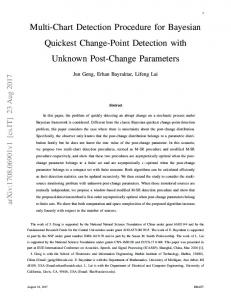
60

Optimal Shiryaev Robust Shiryaev

50

ADD →

40 30 20 10 0 0

Fig. 1.

0.5

1

1.5 θ→

2

2.5

3

Comparison of robust and non-robust Shiryaev tests for α = 0.001 for the Gaussian mean shift example.

exact minimax result does not hold for the robust sequential detection problem in general. He provided examples where the expected stopping times of the SPRT designed with respect to the LFDs are not least favorable under the LFDs. This is similar to the reason why the robust Shiryaev test is not optimal for the Bayesian problem when P0 is not a singleton as explained above. IV. S OME

EXAMPLES AND SIMULATION RESULTS

A. Gaussian mean shift Here we consider a simple example to illustrate the results. Assume ν0 is known to be a standard Gaussian distribution with mean zero and unit variance, so that P0 is a singleton. Let P1 be the collection of Gaussian distributions with means from the interval [0.1, 3] and unit variance. P0 = {N (0, 1)} P1 = {N (θ, 1) : θ ∈ [0.1, 3]}

(17)

It is easily verified that (P0 , P1 ) is jointly stochastically bounded by (ν 0 , ν 1 ) given by ν 0 ∼ N (0, 1),

ν 1 ∼ N (0.1, 1).

1) Bayesian criterion: We simulated the Bayesian and robust Bayesian change detection tests for this problem assuming a geometric prior distribution for the change-point with parameter 0.1 and a false alarm constraint of α = 0.001. From the performance curves plotted in Figure 1, we can see that the

June 2, 2010

DRAFT

14

robust Shiryaev test gives the same average detection delay (ADD) as the optimal Shiryaev test at ν 1 which corresponds to θ = 0.1 in the figure. This is expected since the robust test is identical to the optimal test at ν 1 . For all other values of ν1 ∈ P1 , the performance of the robust test is strictly better than the performance at ν 1 and hence this test is indeed minimax optimal. We also see in Figure 1 that the average delays obtained with the robust test are much higher than those obtained with the optimal test, especially at high values of the mean θ . The probability of false alarm and average detection were estimated via Monte-Carlo simulations with a standard deviation of 0.1% for the estimates. 2) Lorden criterion and comparison with GLR test: Under the Lorden criterion, we compared the performances of three tests - the optimal CUSUM test with known θ , the robust CUSUM test designed with respect to the LFDs, and the CUSUM test based on the Generalized Likelihood Ratio (GLR test) suggested in [4]. The stopping time under the GLR test is given by τGLR = inf{n ≥ 1 : max sup

1≤k≤n ν1 ∈P1

n X

Lν (Xi ) ≥ η}

(18)

i=k

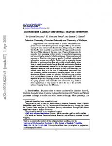
where η is chosen so that the false alarm constraint is met with equality. The GLR test does not require knowledge of θ but still achieves the same asymptotic performance as the optimal CUSUM test with known θ when the false alarm constraint goes to zero for some choices of the uncertainty classes including the example considered above. Figure 2 and Table I shows estimates of the worst-case detection delay (WDD) obtained under the these tests designed for a false alarm constraint of α = 0.001, for various values of θ . These values are estimated using Monte-Carlo simulations. The delay values have a standard deviation lower than 1% and the false alarm value has a standard deviation lower than 3%. From the performance curves in Figure 2 and the values in Table I we see that the GLR test gives better performance than our robust solution at higher values of θ , and is close to optimal at these high values of θ . However, the robust test gives much better performance than the GLR test at the low values of θ . This is expected since the robust solution is minimax optimal and hence is expected to perform better at the unfavorable values of θ . An important difference between the two solutions is that although the robust CUSUM test based on the LFDs admits a simple recursive implementation like we described in (10), the GLR test is in general very complex to implement. This is because the supremum in (18) may be achieved at different values of ν1 for different n. Furthermore, the optimization in (18) may not be easy to solve for general uncertainty

classes - particularly non-parametric classes like the ǫ-uncertainty classes considered next.

June 2, 2010

DRAFT

15

500

Optimal CUSUM Robust CUSUM GLR test

WDD →

400

300

200

100

0 0

Fig. 2.

0.2

0.4

0.6

θ→

0.8

1

Comparison of various tests for false alarm rate of α = 0.001 for the Gaussian mean shift example. TABLE I

D ELAYS OBTAINED USING VARIOUS TESTS UNDER THE L ORDEN CRITERION FOR A

FALSE ALARM RATE OF

θ

Optimal CUSUM

Robust CUSUM

GLR test

0.1

242.7

242.7

496

0.2

111.5

116.8

184

0.4

43.2

55.6

57.2

0.6

23.5

36.3

28.6

1.0

10.5

21.5

12.35

α = 0.001.

B. ǫ-contamination classes We now discuss an example in which the uncertainty class P0 is no longer a singleton. For some scalar ǫ ∈ (0, 1), consider the following ǫ-contamination classes: P0 = {ν0 : ν0 = (1 − ǫ)N (0, 1) + ǫH0 ,

H0 ∈ P(R)}

(19)

P1 = {ν1 : ν1 = (1 − ǫ)N (1, 1) + ǫH1 ,

H1 ∈ P(R)}

(20)

where P(R) is the collection of all probability measures on R and N (µ, σ) denotes the probability measure corresponding to a Gaussian random variable with mean µ and variance σ 2 . In other words, the distributions in uncertainty class Pi are mixtures of a Gaussian distribution with mean i and unit variance, and an arbitrary probability distribution on R with weights given by 1 − ǫ and ǫ respectively. Following the method outlined in [11], we identified LFDs for these uncertainty classes and evaluated

June 2, 2010

DRAFT

16

the performance of the robust test. Let pi denote the density function of a N (µ, 1) random variable and let qi denote the density function of the least favorable distribution from Pi . It is established in [11] that the densities of the LFDs have the following structure,   (1 − ǫ)p (x) if L(x) ≤ b 0 q0 (x) =  1−ǫ p (x) if L(x) > b 1 b   (1 − ǫ)p (x) if L(x) > a 1 q1 (x) =  a(1 − ǫ)p (x) if L(x) ≤ a 0 where L(x) =

(21)

(22)

p1 (x) p0 (x) .

The scalars a and b are identified by the following relation: Z Z 1−ǫ p0 (x)dx + (1 − ǫ) p1 (x)dx = 1 b {x:L(x)≤b} {x:L(x)>b} Z Z p0 (x)dx = 1. p1 (x)dx + a(1 − ǫ) (1 − ǫ) {x:L(x)≤a}

{x:L(x)>a}

In order to compare the performance of the robust test with that of the optimal test we chose the following distributions for H0 and H1 : H0 = N (0, σ0 ), σ0 ∈ [0.1, 10]

H1 = N (1, σ1 ), σ1 ∈ [0.1, 10].

Table II shows the values of the worst-case delay (WDD) obtained when σ0 is kept fixed at σ0 = 1 and σ1 is varied. Shown are the results obtained using the robust CUSUM test as well as the optimal CUSUM test for ǫ = 0.05 and for ǫ = 0.005. We notice that the difference in performance between the robust test and the optimal test is larger for larger values of ǫ. This matches the intuition that the cost of robustness would be higher for a larger uncertainty class of distributions. The delay values and false alarm rates were estimated to have standard deviations lower than 0.1% and 1% respectively. Table III shows the values of worst-case delay obtained under the optimal CUSUM tests when σ1 is kept fixed at σ1 = 1 and σ0 is varied. The delay values and false alarm rates were estimated to have standard deviations lower than 0.1% and 1% respectively. We have not included the delays obtained under the robust test, since the delay of the robust test is invariant with σ0 . The delay obtained under the robust test for ǫ = 0.05 and ǫ = 0.005 are respectively 15.09 and 11.27 as shown in the third row of Table II corresponding to σ1 = 1. V. C ONCLUSION We have shown that for uncertainty classes that satisfy some specific conditions, the optimal change detectors designed for the least favorable distributions are optimal in a minimax sense. This is shown for June 2, 2010

DRAFT

17

TABLE II D ELAYS OBTAINED USING VARIOUS TESTS UNDER THE L ORDEN CRITERION FOR ǫ- UNCERTAINTY CLASSES WITH α = 0.001 AND σ0 = 1. ǫ = 0.05

ǫ = 0.005

σ1

Robust CUSUM

Optimal CUSUM

Robust CUSUM

Optimal CUSUM

0.1

14.77

9.17

11.27

10.38

0.5

14.86

9.12

11.27

10.39

1

15.09

9.08

11.27

10.35

5

15.52

8.78

11.29

10.33

10

15.59

8.65

11.29

10.34

TABLE III D ELAYS OBTAINED USING THE OPTIMAL CUSUM TEST FOR ǫ- UNCERTAINTY CLASSES WITH α = 0.001 σ0

Optimal CUSUM for ǫ = 0.05

Optimal CUSUM for ǫ = 0.005

0.1

10.56

10.55

0.5

10.50

10.52

1

10.44

10.56

5

10.02

10.58

10

9.85

10.59

AND

σ1 = 1.

the Lorden criterion, the Shiryaev-Roberts-Pollak criterion, and Shiryaev’s Bayesian criterion. However, robustness comes at a potential cost. The optimal stopping rule designed for the LFDs may perform quite sub-optimally for other distributions from the uncertainty class when compared with the optimal performance that can be obtained in the case where these distributions are known exactly. Using an asymptotic analysis, we have also obtained an analytic upper bound on this cost of robustness for the robust solution under the Lorden criterion. Nevertheless for some parameter ranges our robust test obtains significant performance improvement over the CUSUM test designed for the Generalized Likelihood Ratio statistic, which is a benchmark for the composite quickest change detection problem. Our robust solution also has the added advantage that it can be implemented in a simple recursive manner, while the GLR test does not admit a recursive solution in general, and may require the solution to a complex non-convex optimization problem at every time instant.

June 2, 2010

DRAFT

18

A PPENDIX A. Proof of Lemma III.1 We prove this claim by induction. For n = 1, the claim holds because if h : R 7→ R is a non-decreasing continuous function we have, P(h(U1 ) ≥ t) = P(U1 ≥ sup{x : h(x) < t} ≥ P(V1 ≥ sup{x : h(x) < t} = P(h(V1 ) ≥ t). N Assume the claim is true for n = N and now consider n = N + 1. For any fixed xN 1 ∈ R , since the

function h is non-decreasing in each of its components, it follows by the proof for n = 1 that, h(x1 , x2 , . . . , xN , UN +1 ) ≻ h(x1 , x2 , . . . , xN , VN +1 ).

(23)

We further have, P(h(U1 , U2 , . . . , UN +1 ) ≥ t) Z N = fU1N (xN 1 )P(h(x1 , x2 , . . . , xN , UN +1 ) ≥ t)dx1 Z N ≥ fU1N (xN 1 )P(h(x1 , x2 , . . . , xN , VN +1 ) ≥ t)dx1 ˜2 , . . . , U ˜N , VN +1 ) ≥ t) = P(h(U˜1 , U Z ˜2 , . . . , U ˜N , y) ≥ t)dy = fVN +1 (y)P(h(U˜1 , U Z ≥ fVN +1 (y)P(h(V1 , V2 , . . . , VN , y) ≥ t)dy

(24) (25)

(26)

= P(h(V1 , V2 , . . . , VN +1 ) ≥ t).

˜i appearing in (25) are random variables with exact where (24) is obtained via (23). The variables U

same statistics as Ui and independent of Vi ’s. The inequality of (26) is obtained by using the induction hypothesis for n = N . Thus we have shown that, h(U1 , U2 , . . . , UN +1 ) ≻ h(V1 , V2 , . . . , VN +1 )

which proves the lemma by the principle of mathematical induction.

June 2, 2010

⊔ ⊓

DRAFT

19

B. Proof of Theorem III.2 Proof: Suppose P0 and P1 satisfy the conditions of the theorem. Since the CUSUM test is optimal for known distributions, it is clear that the test given in (9) is optimal when the pre- and post-change distributions are ν 0 and ν 1 , respectively. Hence, it suffices to show that the values of WDD(τC∗ ) and FAR(τC∗ ) obtained under any ν0 ∈ P0 and any ν1 ∈ P1 , are no higher than their respective values when the pre- and post-change distributions are ν 0 and ν 1 . We use Yi∗ to denote the random variable L∗ (Xi ) when the pre-change and post-change distributions of the observations from the sequence {Xi : i = 1, 2, . . .} are ν 0 and ν 1 , respectively, and Yiν to denote the random variable L∗ (Xi ) when the pre- and post-change distributions are ν0 and ν1 , respectively. We first prove the theorem for a special case. Case 1: P0 is a singleton given by P0 = {ν0 }. Clearly, in this case ν 0 = ν0 and (8) is met trivially. Furthermore, in this case, the false alarm constraint is also met trivially since the false alarm rate obtained by using the stopping rule τC∗ is independent of the true value of the post-change distribution. Fix the change-point to be λ. Now, to complete the proof for the scenario where P0 is a singleton, we will show that for all λ ≥ 1, E∗λ [(τC∗ − λ + 1)+ |Fλ−1 ] ≻ Eνλ [(τC∗ − λ + 1)+ |Fλ−1 ]

(27)

which will establish that the value of WDD(τC∗ ), obtained under any ν1 ∈ P1 , is no higher than the value when the true post-change distribution is ν 1 . Since we now have ν 0 = ν0 , both Yi∗ and Yiν have the same distributions for i < λ and hence we assume without loss of generality that for all i < λ, Yi∗ = Yiν with probability one. Under this assumption, we will show that for all integers N ≥ 0, the following relation holds with probability one, P∗λ ((τC∗ − λ + 1)+ ≤ N |Fλ−1 ) ≤

(28)

Pνλ ((τC∗ − λ + 1)+ ≤ N |Fλ−1 ),

which will then establish (27). Since τC∗ is a stopping time, the event {(τC∗ − λ + 1)+ ≤ 0} is Fλ−1 measurable. Hence, with probability one, (28) holds with equality for N = 0. Now it suffices to verify (28) for N ≥ 1. We know by the stochastic ordering condition on P1 that, Yiν ≻ Yi∗ , for all i ≥ λ

June 2, 2010

(29)

DRAFT

20

Now we have the following equivalence between two events: ( ) n X {τC∗ ≤ N } = max max L∗ (Xi ) ≥ η 1≤n≤N 1≤k≤n

=

(

max

1≤k≤n≤N

It is easy to see that the function, f (x1 , . . . , xN ) ,

n X

i=k ∗

L (Xi ) ≥ η

i=k

max

1≤k≤n≤N

n X

)

.

xi

i=k

is continuous and non-decreasing in each of its components as required by Lemma III.1. Hence for N ≥ 1, the following hold with probability one: P∗λ ((τC∗ − λ + 1)+ ≤ N |Fλ−1 ) =

P∗λ (τC∗ ≤ N + λ − 1|Fλ−1 )

=

Pλ (f (Y1∗ , . . . , YN∗ +λ−1 ) ≥ η|Fλ−1 )

≤

Pλ (f (Y1ν , . . . , YNν +λ−1 ) ≥ η|Fλ−1 )

=

Pνλ (τC∗ ≤ N |Fλ−1 )

=

Pνλ ((τC∗ − λ + 1)+ ≤ N |Fλ−1 )

where the inequality follows from Lemma III.1 and (29), using the fact that f is a non-decreasing function with respect to its last N arguments and the fact that Yiν = Yi∗ for i < λ. Thus, for all integers N ≥ 0, (28) holds with probability one and hence (27) is satisfied. This proves the result for the case where P0 is a singleton. Case 2: P0 is any class of distributions satisfying (8). Suppose that the change does not occur. Then we know by the stochastic ordering condition on P0 that, Yi∗ ≻ Yiν for all i. It follows by Lemma III.1 that, P∗∞ (τC∗ ≤ N ) = P∞ (f (Y1∗ , . . . , YN∗ ) ≥ η) ≥ P∞ (f (Y1ν , . . . , YNν ) ≥ η) = Pν∞ (τC∗ ≤ N )

Since the above relation holds for all N ≥ 1, we have Eν∞ (τC∗ ) ≥ E∗∞ (τC∗ ) =

1 α

(30)

and hence the value of FAR(τC∗ ) is no higher than α for all values of ν0 ∈ P0 and ν1 ∈ P1 . June 2, 2010

DRAFT

21

Now suppose the change-point is fixed at λ. A useful observation is that for any given stopping rule τ and fixed post-change distribution ν1 , the random variable Eνλ0 ,ν1 [(τ − λ + 1)+ |Fλ−1 ] is a fixed deterministic function of the random observations (X1 , . . . , Xλ−1 ), irrespective of the distribution ν0 . Thus the essential supremum of this random variable depends only on the support of ν0 . Applying this observation to the stopping rule τC∗ , and using the relation (8), we have for all ν0 ∈ P0 , ν1 ∈ P1 , ess sup Eλν0 ,ν1 [(τC∗ − λ + 1)+ |Fλ−1 ] ess sup Eλν 0 ,ν1 [(τC∗ − λ + 1)+ |Fλ−1 ].

≤

We also know from Case 1 above that for all ν1 ∈ P1 , ess sup Eλν 0 ,ν1 [(τC∗ − λ + 1)+ |Fλ−1 ] ≤

ess sup E∗λ [(τC∗ − λ + 1)+ |Fλ−1 ].

Taking the supremum over λ ≥ 1, it follows from the above two relations that the value of WDD(τC∗ ) under any pair of distributions (ν0 , ν1 ) ∈ P0 × P1 is no larger than that under (ν 0 , ν 1 ). Thus τC∗ solves the robust problem (4). C. Proof of Theorem III.3 ν ∗ ,η,ψη

∗ := τ Proof: Let τSRP SRP

denote the SRP stopping rule defined with respect to the LFDs (ν0 , ν 1 )

satisfying the asymptotic optimality property of (13) as mentioned in the statement of the theorem. It is easy to see that for any integers λ ≥ 1 and N ≥ 1, we have ∗ ∗ − λ ≤ N |τSRP ≥ λ, R0∗ = r) Pνλ (τSRP

=

∗ − λ ≤ N } ∩ {τ ∗ ≥ λ}|R∗ = r) Pνλ ({τSRP SRP 0 ∗ ≥ λ|R∗ = r) Pνλ (τSRP 0

where R0∗ denotes the random variable with distribution ψη used for initializing the iteration in (11). We follow the same steps as in the proof of Theorem III.2. Let Yiν denote the random variable L∗ (Xi ) when ∗ is a stopping time the the pre-change and post-change distributions are ν0 and ν1 respectively. Since τSRP ∗ ≥ λ} is measurable with respect to the pre-change observations and hence we can represent event {τSRP

this event as, ∗ ν {τSRP ≥ λ} = {(Y1ν , Y2ν , . . . , Yλ−1 ) ∈ T} ∗ where T is the set of pre-change trajectories corresponding to the event {τSRP ≥ λ}. Hence, for any

r ∈ R+ , we can express the conditional probability as ∗ ∗ Pνλ (τSRP − λ ≤ N |τSRP ≥ λ, R0∗ = r) R ∗ ∗ ν ν ν ν ν ν (31) T Pλ (ft (Yλ , Yλ+1 , . . . , YRλ+N ) ≥ g(t, N, η)|R0 = r)Pλ ((Y1 , Y2 , . . . , Yλ−1 ) ∈ dt|R0 = r) = ν ν ν ∗ T Pλ ((Y1 , Y2 , . . . , Yλ−1 ) ∈ dt|R0 = r) June 2, 2010

DRAFT

22

such that for all t ∈ T , the function ft : RN −λ+1 7→ R satisfies the requirements of Lemma III.1, and g(t, N, η) is some real-valued function. The exact form of function ft can be obtained from the iterations

of (11) used to define the SRP stopping rule of (12). We note that in (31) the post-change distribution ν1 affects only the first term under the integral in the numerator. Thus, it follows by applying Lemma

III.1 that ∗ ∗ ≥ λ, R0∗ = r) − λ ≤ N |τSRP P∗λ (τSRP

(32)

∗ ∗ ≤ Pνλ (τSRP − λ ≤ N |τSRP ≥ λ, R0∗ = r)

for all ν1 ∈ P1 . Hence it further follows that, ∗ ∗ ∗ ∗ sup Eνλ (τSRP ≥ λ). − λ|τSRP ≥ λ) = E∗λ (τSRP − λ|τSRP

(33)

ν1 ∈P1

We also observe that for any stopping rule τ that satisfies the false alarm constraint FAR(τ ) ≤ α, we have, sup sup Eνλ (τ − λ|τ ≥ λ)

ν1 ∈P1 λ≥1

≥ sup E∗λ (τ − λ|τ ≥ λ) λ≥1

∗ ∗ ≥ sup E∗λ (τSRP − λ|τSRP ≥ λ) + o(1) λ≥1

∗ ∗ = sup sup Eνλ (τSRP − λ|τSRP ≥ λ) + o(1) ν1 ∈P1 λ≥1

∗ satisfies the asymptotic optimality of (13) when where the second relation follows from the fact that τSRP

the true post-change distribution is ν 1 , and the last equality follows from (33). This completes the proof of the theorem. ∗ is used when P is not a singleton, the crucial step We note that if the robust SRP stopping rule τSRP 0

of (32) does not hold for ν0 6= ν 0 and ν1 = ν 1 . Thus our proof of optimality of the robust SRP stopping rule does not hold when the pre-change distribution is unknown. D. Proof of Theorem III.4 Proof: The proof is very similar to that of Case 1 in Theorem III.2. Since the Shiryaev test is optimal for known distributions, it is clear that the test given in (16) is optimal under the Bayesian criterion when the post-change distribution is ν 1 . Also from the definition of PFA(τS∗ ) it is clear that the probability of false alarm depends only on the pre-change distribution and hence the constraint in (6) is met by the stopping time τS∗ . Hence, it suffices to show that the value of ADD(τS∗ ) obtained under any ν1 ∈ P1 , is no higher than the value when the true post-change distribution is ν 1 . June 2, 2010

DRAFT

23

Let us first fix Λ = λ. We know by the stochastic ordering condition that conditioned on Λ = λ, for all i ≥ λ, we have Yiν ≻ Yi∗ where Yi∗ and Yiν are as defined in the proof of Theorem III.2. As before, the function, f ′ (x1 , . . . , xN ) , max log 1≤n≤N

n X k=1

! n X πk exp( xi ) i=k

is continuous and non-decreasing in each of its components as required by Lemma III.1. Using these facts, we can show the following by proceeding exactly as in the proof of Theorem III.2: Conditioned on Λ = λ, E∗λ ((τS∗ − λ)+ |Fλ−1 ) ≻ Eνλ ((τS∗ − λ)+ |Fλ−1 ).

Thus, we have E∗λ ((τS∗ − λ)+ ) ≥ Eνλ ((τS∗ − λ)+ ) and by averaging over λ, we get, E∗ ((τS∗ − Λ)+ ) ≥ Eν ((τS∗ − Λ)+ ).

R EFERENCES [1] J. Unnikrishnan, V. V. Venugopal, and S. Meyn, “Least favorable distributions for robust quickest change detection,” in Proc. of 2009 IEEE International Symposium on Information Theory, Seoul, Korea, 2009. [2] E. S. Page, “Continuous inspection schemes,” Biometrika, vol. 41, pp. 100–115, 1954. [3] G. V. Moustakides, “Optimal stopping times for detecting changes in distributions,” Ann. Statist., vol. 14, no. 4, pp. 1379–1387, Dec. 1986. [4] G. Lorden, “Procedures for reacting to a change in distribution,” Ann. Math. Statist., vol. 42, no. 6, pp. 1897–1908, 1971. [5] M. Pollak, “Optimal detection of a change in distribution,” Ann. Statist., vol. 13, no. 1, pp. 206–227, 1985. [6] A. N. Shiryaev, Optimal Stopping Rules.

New York: Springer-Verlag, 1978.

[7] A. G. Tartakovsky, Sequential Methods in the Theory of Information Systems.

Moscow: Radio i Svyaz’, 1991.

[8] M. Basseville and I. Nikiforov, Detection of Abrupt Changes: Theory and Applications. Englewood Cliffs, NJ: PrenticeHall, 1993. [9] B. E. Brodsky and B. Darkhovsky, Nonparametric Methods in Change-Point Problems.

Dordrecht: Kluwer, 1993.

[10] A. N. Shiryaev, “On optimum methods in quickest detection problems,” Theory of Prob. and App., vol. 8, pp. 22–46, 1963. [11] P. J. Huber, “A robust version of the probability ratio test,” Ann. Math. Statist., vol. 36, pp. 1753–1758, 1965. [12] P. X. Quang, “Robust sequential testing,” Ann. Statist., vol. 13, no. 2, pp. 638–649, June 1985. [13] R. Crow and S. Schwartz, “On robust quickest change detection procedures,” in Proc., IEEE International Symposium on Information Theory, Trondheim, Norway, 1994, p. 258. [14] H. V. Poor and O. Hadjiliadis, Quickest Detection.

Cambridge, UK: Cambridge University Press, 2009.

[15] A. G. Tartakovsky and A. Polunchenko, “Quickest changepoint detection in distributed multisensor systems under unknown parameters,” in Proc., 11th International Conference on Information Fusion, Cologne, Germany, July 2008. [16] L. Gordon and M. Pollak, “A robust surveillance scheme for stochastically ordered alternatives,” Ann. Statist., vol. 23, no. 4, pp. 1350–1375, 1995. June 2, 2010

DRAFT

24

[17] T. Lai, “Sequential analysis: some classical problems and new challenges,” Stat. Sin., vol. 11, pp. 303–408, 2001. [18] D. Siegmund and E. S. Venkatraman, “Using the generalized likelihood ratio statistic for sequential detection of a changepoint,” Ann. Statist., vol. 23, no. 1, pp. 255–271, 1995. [19] B. Brodsky and B. Darkhovsky, “Asymptotically optimal sequential change-point detection under composite hypotheses,” in Decision and Control, 2005 and 2005 European Control Conference. CDC-ECC ’05. 44th IEEE Conference on, Dec. 2005, pp. 7347–7351. [20] P. J. Huber and V. Strassen, “Minimax tests and the neyman-pearson lemma for capacities,” Ann. Statist., vol. 1, no. 2, pp. 251–263, 1973. [21] V. V. Veeravalli, T. Bas¸ar, and H. V. Poor, “Minimax robust decentralized detection,” IEEE Trans. Inform. Theory, vol. 40, no. 1, pp. 35–40, Jan. 1994. [22] H. Poor, “Robust decision design using a distance criterion,” IEEE Transactions on Information Theory, vol. 26, no. 5, pp. 575–587, Sept. 1994. [23] B. C. Levy, Principles of Signal Detection and Parameter Estimation. [24] A. Wald, Sequential Analysis.

New York: Springer, 2008.

New York: Wiley, 1947.

[25] A. S. Polunchenko and A. G. Tartakovsky, “On optimality of the shiryaev-roberts procedure for detecting a change in distribution,” December 2009, to appear in the Annals of Statistics.

June 2, 2010

DRAFT