Nov 6, 2017 - and (a) is due to the Boole's inequality [19] and (b) is due to Markov's inequality [20] and the fact that Eâ[Î(k, v1,d)] = 1. By choosing m = b α.
Quickest Change Detection under Transient Dynamics: Theory and Asymptotic Analysis Shaofeng Zou*, Georgios Fellouris*† , Venugopal V. Veeravalli*♮ † *Coordinated Science Lab,
♮
ECE Department, † Department of Statistics
University of Illinois at Urbana-Champaign
arXiv:1711.02186v1 [math.ST] 6 Nov 2017
Email: {szou3, fellouri, vvv}@illinois.edu Abstract The problem of quickest change detection (QCD) under transient dynamics is studied, where the change from the initial distribution to the final persistent distribution does not happen instantaneously, but after a series of transient phases. The observations within the different phases are generated by different distributions. The objective is to detect the change as quickly as possible, while controlling the average run length (ARL) to false alarm, when the durations of the transient phases are completely unknown. Two algorithms are considered, the dynamic Cumulative Sum (CuSum) algorithm, proposed in earlier work, and a newly constructed weighted dynamic CuSum algorithm. Both algorithms admit recursions that facilitate their practical implementation, and they are adaptive to the unknown transient durations. Specifically, their asymptotic optimality is established with respect to both Lorden’s and Pollak’s criteria as the ARL to false alarm and the durations of the transient phases go to infinity at any relative rate. Numerical results are provided to demonstrate the adaptivity of the proposed algorithms, and to validate the theoretical results.
1
Introduction
In the problem of quickest change detection (QCD), a decision maker obtains observations sequentially, and at some unknown time (change-point), an event occurs and causes the distribution of the subsequent observations to undergo a change. The objective of the decision maker is to find a stopping rule that detects the change as quickly as possible, subject to a constraint on the false alarm rate. In classical QCD formulations [3–6], the statistical behavior of the samples is characterized by one pre-change distribution and one post-change distribution, which generate the samples before and after the change-point respectively. However, there are many practical applications with more involved statistical behavior after the change-point. For example, when a line outage occurs in a power system, the system goes through multiple transient phases before entering a persistent phase [2]. Motivated by this type of applications, in this work we study the problem of QCD under transient post-change dynamics, in which the pre-change distribution does not change to the persistent The material in this paper was presented in part at the IEEE International Symposium on Information Theory (ISIT), Aachen, Germany, June 2017 [1]. The work of S. Zou and V. V. Veeravalli was supported in part by the National Science Foundation (NSF) under grants CCF 16-18658 and ECCS 14-62311, and by the Air Force Office of Scientific Research (AFOSR) under grant FA9550-16-1-0077, through the University of Illinois at Urbana-Champaign. The work of G. Fellouris was supported by the NSF under grant CIF 15-14245, through the University of Illinois at Urbana-Champaign.
1
distribution instantaneously, but after a number of transient phases. Within the transient and persistent phases, the observations are generated by distributions different from the initial one, and the problem is to detect the change as soon as possible, either during a transient phase or during the persistent phase. As a result, this problem is fundamentally different from the problem of detecting transient changes, studied in [7] and [8], in which the system goes back to its pre-change mode after a single transient phase, and where it is only possible to detect the change within the transient phase. A special case of the QCD problem under transient dynamics is studied in [9], where there is only one transient phase that lasts for a single observation. For this problem, a generalization of Page’s Cumulative Sum (CuSum) algorithm [10] is proposed and shown to be optimal under Lorden’s criterion [11]. A Bayesian formulation is proposed in [12], in which it is assumed that there is an arbitrary, yet known, number of transient phases, whose durations are geometrically distributed. The proposed algorithm in [12] is a generalization of the Shiryaev-Roberts rule [13, 14]. A nonBayesian formulation is considered in [2], where it is assumed that the durations are deterministic and completely unknown. The proposed algorithm in [2] is a generalization of Page’s CuSum test, called the dynamic CuSum (D-CuSum) algorithm. The algorithms in [2] and [12] are shown to admit a recursive structure, but are not supported by any theoretical performance analysis. In this paper, as in [2], we do not make any prior assumptions regarding the transient phases, and we assume that the change-point is deterministic and unknown. We consider the average run length (ARL) to false alarm when the system is operating under the pre-change mode. In the post-change mode, we are interested in the worse-case average detection delay (WADD) as defined by Lorden [11] and Pollak [15]. Our goal is to find a stopping rule that minimizes the WADD subject to a constraint on the ARL. We analyze the performance of the D-CuSum algorithm in [2]. In addition to the D-CuSum algorithm, we further construct a weighted modification of it, which also admits a recursive structure, and analyze its performance. More specifically, we establish the asymptotic optimality of the two algorithms with respect to both Lorden’s [11] and Pollak’s [15] criteria. We note that the post-change distribution in our formulation is composite, as it is determined by the unknown durations of the transient phases. As a result, the proposed problem falls into the framework of QCD with composite post-change distributions [16–18]. However, our work differs from this setup in three major ways. First, thanks to the special structure of our problem, the proposed detection statistics enjoy recursions, which is not typically the case in [16–18]. Second, our asymptotic analysis is novel in that it requires not only the ARL to false alarm, but also the parameters of the post-change distribution (transient durations) to go to infinity. Third, the distribution of the samples within each phase can be arbitrary (may not belong to an exponential family), and the parameters of the post-change distribution (transient durations) are discrete and do not belong to a compact parameter space. The D-CuSum algorithm in [2] was derived by reformulating the QCD problem as a dynamic composite hypothesis testing problem, which conducts a hypothesis test at each time instant k, for 1 ≤ k ≤ ∞, until a stopping criterion is met. At each time k, the null hypothesis corresponds to the case that the change from the pre-change distribution has not occurred yet, and the alternative hypothesis corresponds to the case that the change has occurred. Under the null hypothesis, all samples are distributed according to the pre-change distribution; under the alternative hypothesis, the distribution of the samples up to time k depends on the unknown change-point and durations of the transient phases, and is thus composite. The test statistic at time k is the generalized likelihood
2
ratio between the two hypotheses, and the corresponding stopping rule is obtained by comparing the test statistic against a pre-specified threshold. In this paper, we revisit this algorithm and analyze its performance. However, it is difficult to obtain a lower bound on its ARL in general, and one has to numerically choose the threshold to control the ARL. Motivated by the need for a control of the ARL without resorting to simulations, we propose the weighted D-CuSum (WD-CuSum) algorithm. This algorithm is a variation of the D-CuSum algorithm. The test statistic at time k is a weighted generalized likelihood ratio between the two hypotheses described above. The key idea is that instead of taking a maximum likelihood approach with respect to the unknown composite alternative hypothesis as in the D-CuSum algorithm, we take a mixture approach, and then replace the sum in the mixture with a max in order to obtain a recursive structure for the resulting algorithm. For this test, we derive a lower bound on the ARL, which may be used to set the threshold to satisfy any prescribed lower bound on the ARL. To analyze the asymptotic performance of the D-CuSum and the WD-CuSum algorithms, we consider an asymptotic regime in which the durations of the transient phases go to infinity with the prescribed lower bound on the ARL. We note that if the durations of the transient phases are treated as finite as the ARL goes to infinity, then the information from the transient phases is asymptotically negligible. We first develop an asymptotic universal lower bound on the WADD. Then, we derive asymptotic upper bounds on the WADD for both the D-CuSum and the WD-CuSum algorithms, which match with the asymptotic lower bound and demonstrate that both algorithms are adaptive to the unknown transient durations. This further implies that the WD-CuSum algorithm is optimal with respect to both Lorden’s and Pollak’s criteria [11,15], up to a first-order asymptotic approximation, as the ARL and the transient durations go to infinity at any possible relative rate. The same results are also obtained for the D-CuSum algorithm, under a certain condition that allows for the control of the ARL to false alarm. Numerical results are provided to demonstrate the performance of the proposed algorithms and to validate our theoretical assertions. We show that both the D-CuSum and the WD-CuSum algorithms utilize the information collected from the transient phases to make a timely decision about the change. Furthermore, both algorithms are adaptive to the unknown transient durations. A comparison of the D-CuSum and the WD-CuSum algorithms suggests that they perform similarly. For the issue of choosing weights for the WD-CuSum algorithm, we propose a heuristic approach, based on balancing the performance within the transient and persistent phases. The remainder of this paper is organized as follows. In Section 2, we formulate the problem mathematically. In Section 3, we introduce the D-CuSum and the WD-CuSum algorithms, and establish lower bounds on their ARL to false alarm. In Section 4, we demonstrate the asymptotic optimality of both algorithms. In Section 5, we present the numerical results and propose a heuristic approach of choosing weights for the WD-CuSum algorithm. Finally, in Section 6, we provide some concluding remarks.
2
Problem Model
Consider a sequence of independent random variables {Xk }∞ k=1 , observed sequentially by a decision maker. At an unknown change-point v1 , an event occurs and {Xk }∞ k=v1 undergoes a change in distribution from the initial distribution, f0 . It is assumed that this change goes through L − 1 3
transient phases before entering a persistent phase. Each phase i begins with an unknown starting point vi , and the observations within this phase are generated by a known distribution fi , for 1 ≤ i ≤ L. The duration of i-th transient phase is denoted by di = vi+1 − vi , for 1 ≤ i ≤ L − 1. More specifically, the observations are distributed as follows: Xk ∼ fi , if vi ≤ k < vi+1 ,
(1)
for 0 ≤ i ≤ L, where v0 = 1, v1 ≤ v2 ≤ · · · ≤ vL , and vL+1 = ∞. We assume that L is known in advance and so are the densities fi , 0 ≤ i ≤ L. The change point v1 and the vector of transient durations d = {di , 1 ≤ i ≤ L − 1} are assumed to be deterministic and completely unknown. The goal is to detect the change reliably and quickly based on the sequentially acquired observations. That is, if Fk is the σ-algebra generated by the first k observations, i.e., Fk = σ(X1 , . . . , Xk ), where k = 1, 2, . . ., we want to find a {Fk }k∈N -stopping time that achieves “small” detection delay, while controlling the rate of false alarms. We use Pdv1 to denote the probability measure with the change-point at v1 and the vector of transient durations d, and Edv1 to denote the corresponding expectation. Moreover, we use P∞ and E∞ to denote the probability measure and the corresponding expectation when v1 = ∞, i.e., there is no change. For any stopping time τ , we define the ARL to false alarm and the WADD under Pollak’s criterion [15] as follows: ARL(τ ) =E∞ [τ ], JPd (τ )
= sup v1 ≥1
(2)
Edv1 [τ
− v1 |τ ≥ v1 ].
(3)
We are interested in stopping times that control the expected time to false alarm above a userspecified level, γ > 1, i.e., in Cγ = {τ : ARL(τ ) ≥ γ}. The goal is to design stopping rules that minimize JPd (τ ) subject to this constraint on the ARL: inf JPd (τ ).
(4)
τ ∈Cγ
We are also interested in Lorden’s criterion [11], where the WADD is defined as JLd (τ ) = sup ess sup Edv1 [(τ − v1 )+ |X1 , . . . , Xv1 −1 ],
(5)
v1 ≥1
where (τ − v1 )+ = max{τ − v1 , 0}. R dfi to denote the Kullback-Leibler (KL) divergence between fi and f0 , which We use Ii = fi log df 0 is assumed to be positive and finite, for i = 1, . . . , L. We set Zi (Xk ) = log
fi (Xk ) , f0 (Xk )
(6)
i.e., Zi (Xk ) the log-likelihood ratio between fi and f0 for sample Xk , i = 1, . . . , L, k = 1, 2, . . .. Moreover, we set Λi [k1 , k2 ] =
kY k2 2 −1 Y fi (Xj ) fi (Xj ) and Λi [k1 , k2 ) = . f0 (Xj ) f0 (Xj )
(7)
j=k1
j=k1
We denote the largest integer P 2that is smaller than Qn2x as ⌊x⌋, and the smallest integer that is larger than x as ⌈x⌉. We define nj=n X = 0 and j j=n1 Xj = 1 if n1 > n2 . We denote x = o(1), 1 as c → c0 if ∀ǫ > 0, ∃δ > 0, s.t., |x| ≤ ǫ if |c − c0 | < δ. We denote g(c) ∼ h(c) as c → c0 , if (c) = 1. limc→c0 fg(c) 4
3
The Algorithms
In this section, we introduce the proposed algorithms, show that they admit simple recursive structures, and further obtain (non-asymptotic) lower bounds on their ARL to false alarm. The QCD problem can be reformulated as a dynamic composite hypothesis testing problem as in [2], which is to distinguish the following two hypotheses at each time instant k: H0k : k < v1 , H1k : k ≥ v1 .
(8)
This process stops once a decision in favor of the alternative hypothesis is reached; otherwise, a new sample is taken. Under H0k , the samples X1 , . . . , Xk are distributed according to f0 . The alternative hypothesis H1k is composite, since it depends on v1 , d, which are unknown. Let Γ(k, v1 , d) denote the likelihood ratio of the first k observations, X1 , . . . , Xk , for fixed v1 , d, i.e., Γ(k, v1 , d) =
Pdv1 (X1 , . . . , Xk ) . P∞ (X1 , . . . , Xk )
(9)
When vi ≤ k < vi+1 for some 1 ≤ i ≤ L, Γ(k, v1 , d) = Λi [vi , k] ·
i−1 Y
Λj [vj , vj+1 ).
(10)
j=1
For the special case with L = 2, ( Λ1 [v1 , k], Γ(k, v1 , d1 ) = Λ1 [v1 , v1 + d1 )Λ2 [v1 + d1 , k],
if v1 + d1 > k, if v1 + d1 ≤ k.
(11)
This implies that for a given pair of (v1 , k), there are k − v1 + 2 possible values of Γ(k, v1 , d1 ). Indeed, if we set Aj (k, v1 ) = {j}, for 0 ≤ j ≤ k − v1 , Ak−v1 +1 (k, v1 ) = {k − v1 + 1, k − v1 + 2, . . .},
(12)
then Γ(k, v1 , d1 ) has the same value for every d1 in the same Aj (k, v1 ), and if we denote this value by λ(k, v1 , j), then d1 ∈ Aj (k, v1 ) ⇒ Γ(k, v1 , d1 ) = λ(k, v1 , j),
(13)
where 0 ≤ j ≤ k − v1 + 1. In general, when L ≥ 2, for a given pair of (k, v1 ), there are finitely many possible values of Γ(k, v1 , d), the number of which we denote by n(k, v1 ). Indeed, there is a partition of NL−1 , {Aj (k, v1 ), 0 ≤ j ≤ n(k, v1 ) − 1}, so that Γ(k, v1 , d) has the same value for every d ∈ Aj (k, v1 ), and if we denote this value by λ(k, v1 , j), then d ∈ Aj (k, v1 ) ⇒ Γ(k, v1 , d) = λ(k, v1 , j), where 0 ≤ j ≤ n(k, v1 ) − 1. 5
(14)
3.1
D-CuSum
The D-CuSum [2] detection statistic at time k is the generalized log-likelihood ratio with respect to both v1 and d, for the above hypothesis testing problem: c [k] = max W
max log Γ(k, v1 , d).
(15)
1≤v1 ≤k d∈NL−1
As we explained above, there are finitely many subhypotheses under H1k , which implies that Γ(k, v1 , d) has finitely many values, and the maximization in (15) is over finitely many terms. More specifically, equation (15) is equivalent to the one which takes maximization over {(v1 , . . . , vL ) : 1 ≤ v1 ≤ k, v1 ≤ v2 ≤ · · · ≤ vL ≤ k + 1},
(16)
in which, each tuple of (v1 , . . . , vL ) corresponds to a distinct value of Γ(k, v1 , d). In view of (14), we also have c [k] = max W
max
1≤v1 ≤k 0≤j≤n(k,v1 )−1
log λ(k, v1 , j).
(17)
c [k] against a pre-determined positive The corresponding stopping time is given by comparing W threshold: c [k] > b}. τb(b) = inf{k ≥ 1 : W
(18)
c [k] as the detection Since b > 0, without loss of generality we can adopt the positive part of W statistic. It can be shown that � QL �Qmin{vi+1 −1,k} f (X ) i j j=vi i=1 c [k])+ = (W max log Qk 1≤v1 ≤···≤vL ≤k+1 j=v1 f0 (Xj ) min{v2 −1,k}
=
max
1≤v1 ≤···≤vL ≤k+1
X
Z1 (Xj ) + · · · +
j=v1
k X
ZL (Xj ).
(19)
j=vL
c [k])+ has a recursive structure: It is shown in [2] that (W n o c [k])+ = max Ω b (1) [k], Ω b (2) [k], . . . , Ω b (L) [k], 0 , (W
b (i) [0] = 0 and where for 1 ≤ i ≤ L, we set Ω n o b (i) [k] = max 0, Ω b (1) [k − 1], . . . , Ω b (i) [k − 1] + Zi (Xk ). Ω
(20)
(21)
b (1) [k], . . . , Ω b (L) [k]} depends on X1 , . . . , Xk−1 only Remark 1. The L-dimensional random vector {Ω (1) (L) b b through {Ω [k − 1], . . . , Ω [k − 1]}, thus, it is a Markov process, and regenerates whenever all c [k])+ equals 0 at some k. its components are simultaneously non-positive, or equivalently when (W Moreover, the recursion in (21) implies that the worse-case scenario for the observations up to the c [v1 ] = 0, and consequently for every b > 0 and d we have change-point v1 is when W JLd (b τ (b)) = JPd (b τ (b)) = Ed1 [b τ (b)]. 6
(22)
It is also interesting to point out that unlike the classical CuSum statistic, which we recover by b (1) [k], . . . , Ω b (L) [k]} does not always regenerate under P∞ . Denote by Y the first setting L = 1, {Ω regeneration time, i.e., c [k])+ = 0}. Y = inf{k ≥ 1 : (W
(23)
The following example shows that Y is not always finite.
Example 1. Suppose that L = 2 and f0 , f1 , f2 are chosen such that f0 (x) = 0.5 × 1{x∈[0,2]} , f1 (x) = 0.8 × 1{x∈[0,1]} + 0.2 × 1{x∈(1,2]} , f2 (x) = 0.2 × 1{x∈[0,1]} + 0.8 × 1{x∈(1,2]} .
(24)
Then, max {Z1 (x), Z2 (x)} > 0, ∀x ∈ [0, 2], which implies that for all k ≥ 1, we have pathwise n o c [k])+ = max Ω b (1) [k], Ω b (2) [k], 0 > 0. (W (25) If we assume that the pre- and post-change distributions satisfy the following condition: P∞ (Y > m) ≤ e−αm ,
∀m ≥ 1,
(26)
c [k])+ is regenerative, and the ARL of the D-CuSum where α is any positive constant, then (W algorithm is lower bounded as in the following proposition. See Example 2 for sufficient conditions for (26) to hold. Proposition 1. Consider the QCD problem under transient dynamics described in Section 2. Assume that the pre- and post-change distributions satisfy condition (26). If the D-CuSum algorithm is applied with a threshold b, then the ARL is lower bounded as follows: E∞ [b τ (b)] ≥ o n c [k])+ Proof. Under (26), (W
k≥1
eb 1+
� b L+1 α
.
(27)
is regenerative, which implies that
E∞ [b τ (b)] =
1 E∞ [Y ] ≥ . P∞ (b τ (b) < Y ) P∞ (b τ (b) < Y )
(28)
For any m ≥ 1, P∞ (b τ (b) < Y ) = P∞ (b τ (b) < Y, Y ≤ m) + P∞ (b τ (b) < Y, Y > m) ≤ P∞ (b τ (b) < m) + P∞ (Y > m) ≤ mL+1 e−b + e−αm ,
(29)
7
where the last inequality is due to condition (26) and the following fact: P∞ (b τ (b) < m) � � c [k] > b = P∞ max W 1≤k0 θ(t) + tEf0 [Φ(Xj )] < 0, where h � ��i , θ(t) = log Ef0 exp t Φ(Xj ) − Ef0 [Φ(Xj )]
(32)
(33)
then (26) holds.
For any (v1 , d, k), it follows from (9) and (32) that log Γ(k, v1 , d) ≤
k X
Φ(Xj ).
(34)
j=v1
This further implies that c [k] ≤ max W
1≤v1 ≤k
8
k X
j=v1
Φ(Xj ).
(35)
n o P Let Y ′ = inf k ≥ 1 : max1≤v1 ≤k kj=v1 Φ(Xj ) ≤ 0 . Then by (35), Y ′ ≥ Y . It then follows that P∞ (Y > m)
≤ P∞ (Y ′ > m)
= P∞ max
1≤v1 ≤k
k X
j=v1
Φ(Xj ) > 0, ∀1 ≤ k ≤ m
k X (a) = P∞ Φ(Xj ) > 0, ∀1 ≤ k ≤ m
≤ P∞
= P∞
j=1
m X j=1
Φ(Xj ) > 0
m � X j=1
(b)
≤ e−αm ,
� Φ(Xj ) − E∞ [Φ(Xj )] > −mE∞ [Φ(Xj )]
(36)
where (a) is by applying the following argument recursively: �! \� [ P∞ Φ(X1 ) > 0 Φ(X2 ) > 0 Φ(X1 ) + Φ(X2 ) > 0 = P∞ �
�
Φ(X1 ) > 0
= P∞ Φ(X1 ) > 0
\
\
�[� �! \ Φ(X2 ) > 0 Φ(X1 ) > 0 Φ(X1 ) + Φ(X2 ) > 0
� Φ(X1 ) + Φ(X2 ) > 0 ,
(37)
and (b) is by applying the Chernoff bound [21].
3.2
WD-CuSum
If we take a mixture approach with respect to d, combined with a maximum likelihood approach with respect to v1 , this suggests the following stopping rule: τ ′ (b) = inf{k ≥ 1 : W ′ [k] ≥ b}, where b is a positive threshold and the detection statistic is X Γ(k, v1 , d)g(d) , W ′ [k] = max log 1≤v1 ≤k
(38)
(39)
d∈NL−1
and g is a pmf on NL−1 . In view of (13) and (14), for fixed k and v1 , this mixture is equivalent to a sum over finitely many terms, since there are finitely many values of Γ(k, v1 , d): n(k,v1 )−1 X (40) λ(k, v1 , j)g(Aj (k, v1 )) , W ′ [k] = max log 1≤v1 ≤k
j=0
9
where g(A) =
P
d∈A g(d).
Replacing the sum with a maximum, we obtain
f [k] = max W
max
1≤v1 ≤k 0≤j≤n(k,v1 )−1
which leads to the following stopping rule:
� log λ(k, v1 , j)g(Aj (k, v1 )) ,
f [k] ≥ b}. τe(b) = inf{k ≥ 1 : W
(41)
(42)
We refer to this stopping rule in (42) as the WD-CuSum algorithm. In the following, we focus on τe for a particular choice of g, which yields a recursive structure for f . In particular, if we choose W g(d) =
L−1 Y
ρi (1 − ρi )di ,
(43)
i=1
f [k] (since b > 0), then for some ρi ∈ (0, 1), 1 ≤ i ≤ L − 1, and consider the positive part of W ! QL B i + i=1 f [k]) = (W max log Qk , (44) 1≤v1 ≤···≤vL ≤k+1 j=v1 f0 (Xj ) where for i = 1, . . . , L,
Bi =
min{vi+1 −1,k}
Y
1
{k≥vi+1 } , fi (Xj )(1 − ρi ) ρi
j=vi
with vL+1 = ∞ and ρL = 0.
Following steps similar to those in [2, Appendix], it can be shown that n o f [k])+ = max Ω e (1) [k], . . . , Ω e (L) [k], 0 , (W
where
e (i) [k] = max e Ω(j) [k − 1] + Ω 0≤j≤i
i−1 X ℓ=j
e (0) [k] = 0, for all k, and ρ0 = 1. with Ω
log ρℓ + Zi (Xk ) + log(1 − ρi ), for 1 ≤ i ≤ L,
(45)
(46)
(47)
P Example 3. When L = 2, setting G(x) = k>x g(k), we have ) ( k−ν X1 ′ g(d1 )Λ1 [v1 , v2 )Λ2 [v2 , k] + G(k − ν1 )Λ1 [v1 , k] , W [k] = max log 1≤v1 ≤k
f [k] = max log W 1≤v1 ≤k
(
d1 =0
max
�
max
0≤d1 ≤k−ν1
�) . g(d1 )Λ1 [v1 , v2 )Λ2 [v2 , k], G(k − ν1 )Λ1 [v1 , k]
(48)
Theorem 1. Consider the QCD problem under transient dynamics described in Section 2. Assume that the WD-CuSum algorithm in (42) is applied with threshold b and any ρi ∈ (0, 1), 1 ≤ i ≤ L − 1. Then, the ARL of the WD-CuSum algorithm is lower bounded as follows: 1 E∞ [e τ (b)] ≥ eb . 2 10
(49)
Proof. For every k ∈ N we have f [k] ≤ W ′ [k] W = max log 1≤v1 ≤k
≤ log
k X
X
d∈NL−1
X
v1 =1 d∈NL−1
≡ log R[k],
Γ(k, v1 , d)g(d)
Γ(k, v1 , d)g(d)
(50)
where W ′ [k] is as in (39), and the first inequality follows by the construction of the detection statistics. Note that R[k] is a mixture Shiryaev-Roberts statistics, and therefore {R[k] − k}k≥1 is a martingale under P∞ [22]. Thus, for every b > 0 and k ∈ N we have by Doob’s submartingale inequality [19] that P∞ (e τ (b) ≤ k) � � f = P∞ max W [s] ≥ b 1≤s≤k � � b ≤ P∞ max R[s] ≥ e 1≤s≤k
−b
≤ ke ,
(51)
which implies that E∞ [e τ (b)] = ≥
∞ X
P∞ (e τ (b) > k)
k=0 ∞ X
(1 − ke−b )+
k=0 b
e � � X 1 − ke−b =
≥
k=0 eb
2
.
(52)
Remark 2. The lower bound can be further tightened to eb by using Doob’s optional sampling theorem [23] instead of the submartingale inequality. However, this does not provide order-level improvement. Corollary 2. To guarantee E∞ [e τ (b)] ≥ γ, it suffices to choose b = log γ + log 2 ∼ log γ. Proof. The result follows from Theorem 1.
11
(53)
4
Asymptotic Analysis
In this section we study the asymptotic performance of the proposed algorithms and demonstrate their asymptotic optimality. For our asymptotic analysis to be non-trivial, we let not only the prescribed lower bound on the ARL, γ, go to infinity, but also the transient durations. Indeed, if the latter are fixed as γ goes to infinity, then the CuSum algorithm that detects the change from f0 to fL , completely ignoring the transient phases, can be shown to be asymptotically optimal using the techniques in [16]. Therefore, in order to perform a general and relevant asymptotic analysis, we let d1 , . . . , dL−1 go to infinity with γ. Specifically, we assume that di ∼ ci
log γ , Ii
(54)
where ci ∈ [0, ∞] for every i = 1, . . . , L − 1 and cL = ∞. We start with the case with L = 2, since it captures the essential features of the analysis, and then present the generalization to L > 2.
4.1
Asymptotic Universal Lower Bound on the WADD
Consider the case with L = 2, for which d = d1 . As will be shown in the following, the optimal asymptotic performance depends on whether c1 ≥ 1 or c1 < 1. This dichotomy can be seen in the following asymptotic universal lower bound on the WADD. Theorem 2. Consider the QCD problem under transient dynamics described in Section 2 with L = 2. Suppose that (54) holds, i.e., d1 ∼ c1 log γ/I1 . (i) If c1 ≥ 1, then as γ → ∞, inf JLd1 (τ ) ≥ inf JPd1 (τ ) τ ∈Cγ
τ ∈Cγ
≥
log γ (1 − o(1)); I1
(55)
(ii) if c1 < 1, then as γ → ∞, inf JLd1 (τ ) ≥ inf JPd1 (τ ) τ ∈Cγ τ ∈Cγ � � 1 − c1 c1 ≥ log γ + (1 − o(1)). I2 I1
(56)
Proof. See Appendix B. Theorem 2 suggests that to meet the asymptotic universal lower bound on the WADD, an algorithm should be adaptive to the unknown d1 . The proof of the asymptotic universal lower bound is based on a change-of-measure argument and the Weak Law of Large Numbers for log-likelihood ratio statistics, similarly to [16]. However, a major difference is that when changing measures, the post-change statistic is more complicated, due to the cascading of the transient and persistent distributions. In the proof, a decomposition of the sum of the log-likelihood of the samples is necessary before the application of the Weak Law of Large Numbers. 12
4.2
Asymptotic Upper Bounds on the WADD
We now establish asymptotic upper bounds on the WADD of the proposed algorithms for a threshold b. By the construction of the D-CuSum and the WD-CuSum algorithms in (18) and (42), for any k ≥ 1, f [k] ≤ W c [k], W
(57)
which is due to the fact that the weights in the WD-CuSum algorithm are less than one. Therefore, with the same threshold b, the WD-CuSum algorithm will always stop later than the D-CuSum algorithm. Recall that the WD-CuSum algorithm depends on the parameter ρ1 . When L = 2, f [k])+ = max{Ω e (1) [k], Ω e (2) [k], 0}, (W
where
� �+ e (1) [k] = Ω e (1) [k − 1] + Z1 (Xk ) + log(1 − ρ1 ), Ω n o e (2) [k] = max log ρ1 , Ω e (1) [k − 1] + log ρ1 , Ω e (2) [k − 1] + Z2 (Xk ). Ω
(58)
(59)
As we can observe from (59), the drift of the WD-CuSum algorithm for the samples within the e (2) [k]. To meet transient phase is I1 + log(1 − ρ1 ), and there is a negative constant log ρ1 added to Ω the asymptotic universal lower bound on the WADD (which does not depend on ρ1 ), we need to mitigate the effect of ρ1 on the performance. If we choose ρ1 such that as b → ∞, ρ1 → 0 and
log ρ1 → 0, b
(60)
e.g., ρ1 = 1/b, then the “effective drift” within the transient phase is I1 (1 − o(1)), and the “effective threshold” is b(1 + o(1)), asymptotically. In this way, the effect of the weights on the upper bound is asymptotically negligible. We further assume that there is a constant c′1 ∈ [0, ∞], such that d1 ∼ c′1
b . I1
(61)
If we choose b ∼ log γ, then c1 = c′1 , where c1 is defined in (54). The following theorem characterizes asymptotic upper bounds on the WADD for the WD-CuSum and D-CuSum algorithms. Theorem 3. Consider the QCD problem under transient dynamics described in Section 2 with L = 2. Suppose that (60) and (61) hold. Consider the WD-CuSum algorithm in (42), and the D-CuSum algorithm in (18). (i) If c′1 > 1, then as b → ∞, b (1 + o(1)), I1 b JLd1 (b τ (b)) = JPd1 (b τ (b)) ≤ (1 + o(1)); I1 JLd1 (e τ (b)) = JPd1 (e τ (b)) ≤
13
(62) (63)
(ii) if c′1 ≤ 1, then as b → ∞, � 1 − c′1 c′1 + (1 + o(1)), = ≤b I1 I2 � ′ � c 1 − c′1 JLd1 (b τ (b)) = JPd1 (b τ (b)) ≤ b 1 + (1 + o(1)). I1 I2
JLd1 (e τ (b))
JPd1 (e τ (b))
�
(64) (65)
Proof. See Appendix C. By arguments similar to those in Remark 1, it is clear that the WADD for the D-CuSum and the WD-CuSum algorithms is achieved when v1 = 1 under both Lorden’s and Pollak’s criteria. In f [k] ≤ W c [k], we have addition, since W JLd1 (b τ (b)) = JPd1 (b τ (b)) ≤ JLd1 (e τ (b)) = JPd1 (e τ (b)).
(66)
Thus, in the proof, it suffices to upper bound Ed11 [e τ (b)]. The proof of the asymptotic upper bounds on WADD is based on an argument of partitioning the samples into independent blocks and the Law of Large Numbers for log-likelihood ratio statistics similar to those in [16, Theorem 4]. The major difficulty is due to the more complicated post-change statistic, which is a cascading of the transient and persistent distributions. In the proof, a novel approach of partitioning samples is needed to guarantee large probability of crossing the threshold within each block. Moreover, a decomposition of the sum of log-likelihood of the samples from f1 and f2 , respectively, is also necessary before the application of the Law of Large Numbers. The WADD is upper bounded differently in two regimes, depending on c′1 , which determines the scaling behavior between d1 and b. If d1 is “large”, then the WD-CuSum algorithm stops within the transient phase with high probability, such that the asymptotic upper bound only depends on I1 ; if d1 is “small”, then the WD-CuSum algorithm stops within the persistent phase with high probability, such that the asymptotic upper bound depends on a mixture of I1 and I2 . This is consistent with the insights gained from the asymptotic universal lower bound in Theorem 2.
4.3
Asymptotic Optimality
We are now ready to establish the asymptotic optimality of the proposed rules with respect to both Lorden’s and Pollak’s criteria under every possible post-change regime. Theorem 4. Consider the QCD problem under transient dynamics described in Section 2 with L = 2. (i) If ∃b ∼ log γ so that E∞ [b τ (b))] ≥ γ. Then, as γ, d1 → ∞ according to (54), τ (b)) ∼ inf JPd1 (τ ) JLd1 (b τ (b)) ∼ inf JLd1 (τ ) ∼ JPd1 (b τ ∈Cγ τ ∈Cγ log γ if c1 > 1, I , 1 � � ∼ 1 − c1 c log γ 1 + , if c1 ≤ 1. I1 I2 14
(67)
(ii) Let b ∼ log γ so that E∞ [e τ (b)] ≥ γ. Then, as γ, d1 → ∞ and ρ1 → 0 according to (54) and (60) respectively, τ (b)) ∼ inf JPd1 (τ ) JLd1 (e τ (b)) ∼ inf JLd1 (τ ) ∼ JPd1 (e τ ∈Cγ τ ∈Cγ log γ if c1 > 1, I , 1 � � ∼ c 1 − c1 log γ 1 + , if c1 ≤ 1. I1 I2
(68)
WADD
Proof. The results follow from Proposition 1 and Theorems 1, 2, and 3.
log
Figure 1: A heuristic explanation for the dichotomy in Theorem 4. A heuristic explanation for the dichotomy in Theorem 4 is as follows (see also Fig. 1). If we wish to detect a change from f0 to f1 with ARL γ, we have WADD∼ log γ/I1 (see, e.g., Theorem 1 in [16]). However, we only have d1 samples from f1 within the transient phase. If d1 ≥ log γ/I1 , i.e., c1 ≥ 1, then the problem is similar to one of testing the change from f0 to f1 , and WADD increases when log γ increases with slope 1/I1 , i.e., WADD ∼
log γ . I1
(69)
If d1 < log γ/I1 , i.e., c1 < 1, we then need further information from f2 , and WADD increases when log γ increases with slope 1/I2 . To obtain the overall slope, it then follows that d1 I1 + (WADD − d1 )I2 ≈ log γ,
15
(70)
which implies that log γ − d1 I1 I2 � � 1 − c1 c1 ∼ log γ + . I2 I1
WADD ≈ d1 +
4.4
(71)
Generalization to Arbitrary L
The asymptotic universal lower bound on the WADD can be extended to the case with arbitrary L. Theorem 5. Consider the QCD problem under transient dynamics Pjdescribed in Section 2 with an arbitrary L ≥ 2. Suppose that (54) holds. If h = min{1 ≤ j ≤ L : i=1 ci ≥ 1}, then as γ → ∞ inf JLd (τ ) ≥ inf JPd (τ )
τ ∈Cγ
τ ∈Cγ
≥ log γ
h−1 X i=1
! P ci 1 − h−1 i=1 ci (1 − o(1)). + Ii Ih
(72)
Proof. The proof is a cumbersome but straightforward generalization of the case with L = 2, and is omitted. We further assume that there is a constant c′i ∈ [0, ∞], such that di ∼ c′i
b , I1
(73)
for 1 ≤ i ≤ L − 1. If we choose b ∼ log γ, then ci = c′i , 1 ≤ i ≤ L − 1. Similar to the case with L = 2, we design ρi for the WD-CuSum algorithm such that the effect of the additionally introduced weights is asymptotically negligible. We choose ρi such that as b → ∞, ρi → 0, and
− log ρi → 0, b
(74)
for i = 1, . . . , L − 1. We then obtain the following theorem characterizing asymptotic upper bounds on the WADD of the D-CuSum and the WD-CuSum algorithms. Theorem 6. Consider the QCD problem under transient dynamicsP described in Section 2 with an arbitrary L. Suppose (73) and (74) hold. Let h = min{1 ≤ j ≤ L : ji=1 c′i ≥ 1}, then as γ → ∞ JLd (b τ (b)) = JPd (b τ (b)) ≤ JLd (e τ (b)) = JPd (e τ (b)) ! P h−1 ′ X c′ 1 − h−1 i i=1 ci + (1 + o(1)). ≤b Ii Ih
(75)
i=1
Proof. The proof is a cumbersome but straightforward generalization of the case with L = 2, and is omitted.
16
We are then ready to establish the asymptotic optimality of the proposed algorithms with respect to both Lorden’s and Pollak’s criteria under every possible post-change regime for L ≥ 2. Theorem 7. Consider the QCD problem under transient dynamics described Pj in Section 2 with L ≥ 2. Assume that (54) is satisfied, as γ, d → ∞. Let h = min{1 ≤ j ≤ L : i=1 ci ≥ 1}. (i) If ∃b ∼ log γ such that E∞ [b τ (b))] ≥ γ. Then, as γ → ∞,
τ (b)) ∼ inf JPd (τ ) JLd (b τ (b)) ∼ inf JLd (τ ) ∼ JPd (b τ ∈Cγ τ ∈Cγ ! P h−1 h−1 X ci 1 − c i i=1 ∼ log γ . + Ii Ih
(76)
i=1
(ii) Choose ρi for 1 ≤ i ≤ L − 1 such that (74) is satisfied and b ∼ log γ such that E∞ [e τ (b)] ≥ γ. Then, as γ → ∞, τ (b)) ∼ inf JPd (τ ) JLd (e τ (b)) ∼ inf JLd (τ ) ∼ JPd (e τ ∈Cγ τ ∈Cγ ! P h−1 X ci 1 − h−1 ci i=1 . + ∼ log γ Ii Ih i=1
Proof. The results follow from Proposition 1 and Theorems 1, 5 and 6. A heuristic explanation for the polychotomy for the general case with arbitrary L in Theorem 7 is as follows (see also Fig. 2). If we wish to test a change from f0 to f1 with ARL γ, we have WADD∼ log γ/I1 . If d1 < log γ/I1 , we further need samples from f2 . If d1 I1 + d2 I2 is still less than log γ, we then use samples from f3 . Up to the h-th transient phase, we have collected sufficient number of samples such that h X
di Ii > log γ.
(77)
i=1
To obtain the overall slope, it then follows that h−1 X
di Ii +
WADD −
h−1 X
di
i=1
i=1
!
Ih ≈ log γ,
(78)
which implies that WADD ≈
log γ −
∼ log γ
Ph−1 i=1
di Ii
Ih
1−
Ph−1 i=1
Ih
17
+
ci
h−1 X
di
i=1 h−1 X
+
i=1
ci Ii
!
.
(79)
WADD
Figure 2: A heuristic explanation for the results of the general case with arbitrary L in Theorem 7.
5
Numerical Studies
In this section, we present some numerical results. We focus on the case with L = 2 to illustrate the performance of the algorithms and demonstrate our theoretical assertions. Together with the insights gained from the theoretical results, we also propose a heuristic approach to assign the weights for the WD-CuSum algorithm. In Fig. 3, we plot the evolution paths of the WD-CuSum and D-CuSum algorithms. We choose f0 = N (0, 1), f1 = N (3, 1) and f2 = N (1, 1). We assume that the change happens at v1 = 20 and the persistent phase starts at v2 = 40. We choose ρ1 = 1/1000 for the WD-CuSum algorithm, which is small enough compared to I1 . It can be seen that the values of both the WD-CuSum and D-CuSum algorithms stay close to zero before the change-point v1 and grow after the change-point v1 with different drifts in the transient and persistent phases. Both algorithms are seen to be adaptive to the unknown transient duration d1 . Furthermore, within the transient phase, the WD-CuSum and D-CuSum algorithms have close evolution paths. After v2 , there is a gap of roughly | log ρ1 | between the two evolution paths. These observations reflect the difference between the WD-CuSum and D-CuSum algorithms. For the D-CuSum algorithm, the drift is I1 within the transient phase, and I2 within the persistent phase. Recall that for the WD-CuSum algorithm, the drift within the transient phase is reduced from I1 by | log(1 − ρ1 )|. Since ρ1 is chosen to be small compared to I1 , the change of drift is not significant in the figure. Furthermore, the value of the WD-CuSum statistic is reduced by | log ρ1 | within the persistent phase. Therefore, the difference between the values of the D-CuSum and the WD-CuSum statistics is roughly | log ρ1 | as shown in the figure. We next compare the performance of the WD-CuSum algorithms with different ρ1 and the DCuSum algorithm. The goal is to check how different choices of ρ1 affect the performance of the WD-CuSum algorithm relative to the D-CuSum algorithm. We choose f0 = N (0, 1), f1 = N (0.3, 1) 18
120 D-CuSum WD-CuSum
100
Test Statistic
|log
1
|
80 60 v1=20
40
v2=40
20 0 0
10
20
30
40
50
60
k
Figure 3: Evolution paths of the WD-CuSum and D-CuSum algorithms and f2 = N (−0.3, 1). For the WD-CuSum algorithm, we consider three different choices of ρ1 , i.e., ρ1 = 0.01, 0.02 and 0.04. We choose d1 = 40 and d1 = ∞, and plot the WADD versus the ARL in Fig. 4 and Fig. 5, respectively. Fig. 4 and Fig. 5 show that if the algorithms stop within the transient phase, i.e., WADD≤ d1 , the WD-CuSum algorithm has a better performance than the D-CuSum algorithm. Fig. 4 also shows that if the algorithms stop within the persistent phase, i.e., WADD> d1 , the D-CuSum and the WD-CuSum algorithms have similar performance. In Fig. 4, when the algorithms stop within the persistent phase, i.e., WADD> d1 , the WD-CuSum algorithm has a better performance if ρ1 is larger. This is due to the fact that the value of the WD-CuSum statistic is reduced by | log ρ1 | in the persistent phase, which slows down the detection. With a larger ρ1 , this effect is mitigated, which results in better performance for the WD-CuSum algorithm in the persistent phase. In Fig. 4 and more clearly in Fig 5, when the algorithms stop within the transient phase, i.e., WADD≤ d1 , the WD-CuSum algorithm has a better performance if ρ1 is smaller. This is due to the fact that the drift of the WD-CuSum algorithm is reduced by | log(1 − ρ1 )| in the transient phase, which also slows down the detection. With a smaller ρ1 , this effect is reduced, which results in better performance for the WD-CuSum algorithm in the transient phase. As can be observed in Fig. 4 and Fig. 5, the performance of the WD-CuSum algorithm depends on the choice of ρ1 , but not monotonically. A smaller ρ1 yields a better performance for the WD-CuSum algorithm in the transient phase, and a larger ρ1 yields a better performance for the WD-CuSum algorithm in the persistent phase. However, since d1 is not known in advance, it is not clear in which regime the WD-CuSum algorithm will stop. Therefore, we propose a moderate way to choose ρ1 that balances the performance within the transient and persistent phases. Since the lower bound on the ARL in Theorem 1 does not depends on ρ1 , we choose b ∼ log γ. We choose ρ1 to be small but not too small such that the WD-CuSum algorithm is robust to
19
120
100
WD-CuSum with 1 =0.01 WD-CuSum with 1 =0.02 WD-CuSum with 1 =0.04 D-CuSum
WADD
80
60 D1=40 40
20
0 10 0
10 1
10 2
10 3
10 4
ARL
Figure 4: WADD versus ARL for the WD-CuSum and D-CuSum algorithms with d1 = 40. the unknown d1 , i.e., the WD-CuSum algorithm has a good performance in both the transient and persistent phases. Recall that the drift within the transient phase is reduced from I1 by | log(1−ρ1 )|. From our asymptotic analysis, we would like to have − log(1 − ρ1 ) → 0, as b → ∞. I1
(80)
− log(1 − ρ1 ) ≤ δ1 I1 ,
(81)
Therefore, we let
for some δ1 ∈ (0, 1), such that the drift is reduced by a small fraction of I1 . Furthermore, within the persistent phase the value of the WD-CuSum statistic is reduced by | log ρ1 |. From our asymptotic analysis, we would like to have − log ρ1 → 0, as b → ∞. b
(82)
− log ρ1 ≤ δ2 b,
(83)
Therefore, we let
for some δ2 ∈ (0, 1), such that | log ρ1 | is a small perturbation compared to b. Therefore, ρ1 is chosen such that e−δ2 b < ρ1 < 1 − e−δ1 I1 .
(84)
For example, we let δ1 = δ2 = 0.3. Assume that I1 = 0.045 (as in Fig. 4 and Fig. 5) and the required ARL is 107 . Then we can choose b = log(107 ) and ρ1 ∈ [0.008, 0.134]. 20
120
100
WD-CuSum with 1 =0.01 WD-CuSum with 1 =0.02 WD-CuSum with 1 =0.04 DCuSum
WADD
80
60
40
20
0 10 0
10 1
10 2
10 3
10 4
ARL
Figure 5: WADD versus ARL for the WD-CuSum and D-CuSum algorithms with d1 = ∞.
6
Conclusions
In this paper, we studied a variant of the QCD problem that arises in a number of engineering applications. Our problem formulation captures the scenarios with transient dynamics after a change. We studied two algorithms for this formulation, the D-CuSum and the WD-CuSum algorithms. We established bounds on the ARL to false alarm for these algorithms that can be used to set the thresholds of these algorithms in application settings. We also established the asymptotic optimality of the D-CuSum and the WD-CuSum algorithms up to a first-order asymptotic approximation. Both algorithms admit recursions that facilitate implementation and are adaptive to unknown transient dynamics. We have shown that the asymptotic optimal performance follows a polychotomy as illustrated in Fig. 2. In particular, for the case with only one transient phase, the asymptotic optimal performance follows a dichotomy: if the duration of the transient phase is “large”, then the WADD only depends on the distribution associated with the transient phase; otherwise, the WADD depends on the distributions associated with both the transient and the persistent phases. A possible extension of the problem formulation studied in this paper is a generalization to the case where the observations within each transient phase are not i.i.d. as in the observation model studied by Lai [16]. Another extension is the scenario in which prior statistical knowledge of the change-point and durations of the transients is available. In this case, such prior knowledge should be incorporated into the design of algorithms to improve performance, while taking into account computational efficiency. We also note that the generalization to the case in which the distribution within each transient phase is composite is also of interest in practice, an example of which is 21
the sequentially detection of a propagating event with an unknown propagation pattern in sensor networks.
22
Appendix A
A Useful Lemma
We recall the following useful lemma, which is a slight generalization of the Weak Law of Large Numbers. Lemma 1. [24, Lemma A.1] Suppose random variables Y1 , Y2 , . . . , Yk are i.i.d. on (Ω, F, P) with Pk E[Yi ] = µ > 0, and denote Sk = i=1 Yi , then for any ǫ > 0, as n → ∞, � � max1≤k≤n Sk P − µ > ǫ → 0. (85) n
B
Proof of Theorem 2
Recall from (54) that d1 ∼
c1 log γ I1
for some c1 ∈ [0, ∞]. We define Kγ as follows: log γ c1 ∈ [1, ∞]; I , 1 � � Kγ = 1 − c1 c1 + log γ, c1 ∈ [0, 1). I2 I1
(86)
Fix any small enough ǫ > 0. By Markov’s inequality, we have Edv11 [τ − v1 |τ ≥ v1 ]
� ≥ Pdv11 τ − v1 ≥ (1 − ǫ)Kγ |τ ≥ v1 (1 − ǫ)Kγ .
It then suffices to show
sup Pdv11 (τ − v1 < (1 − ǫ)Kγ |τ ≥ v1 ) → 0 as γ → ∞.
(87)
(88)
τ ∈Cγ
We will consider two cases depending on c1 ≥ 1 or c1 < 1. Case 1 : Consider c1 ≥ 1. Then (1 − ǫ)Kγ < d1 for large γ. We first have for every a > 0, Pdv11 (v1 ≤ τ < v1 + (1 − ǫ)Kγ |τ ≥ v1 ) � � d1 = Pv1 v1 ≤ τ < v1 + (1 − ǫ)Kγ , log Λ1 [v1 , τ ] ≥ a τ ≥ v1 � � d1 + Pv1 v1 ≤ τ < v1 + (1 − ǫ)Kγ , log Λ1 [v1 , τ ] < a τ ≥ v1 � � d1 ≤ Pv1 log Λ1 [v1 , v1 + j] ≥ a τ ≥ v1 max 0≤j nb i) .
(114)
i=cǫ +1
i=1
It then suffices to bound Pd11 (e τ (b) > nb i) for the two regimes, i ≤ cǫ and i > cǫ . We note that the event {e τ (b) > nb i} only depends on the samples X1 , . . . , Xnb i . For 1 ≤ i ≤ cǫ , X1 , . . . , Xnb i are i.i.d. generated from f1 under Pd11 . Therefore, Pd11 (e τ (b) > nb i) � � d1 + f = P1 max (W [k]) ≤ b 1≤k≤nb i � � = Pd11 max max w[k1 , k, v2 ] ≤ b 1≤k≤nb i 1≤k1 ≤v2 ≤k+1
≤
Pd11
(w[(u − 1)nb + 1, unb , d1 + 1] ≤ b, ∀1 ≤ u ≤ i) unb X � Z1 (Xj ) + log(1 − ρ1 ) ≤ b, ∀1 ≤ u ≤ i = Pd11 j=(u−1)nb +1
(a)
=
i Y
u=1 (b)
≤ δi ,
1 Pd11 nb
unb X
j=(u−1)nb +1
� b Z1 (Xj ) + log(1 − ρ1 ) ≤ nb
(115)
where δ can be arbitrarily small for large b, (a) is due to the fact that {X1+(u−1)nb , . . . , Xunb } are independent from {X1+(u′ −1)nb , . . . , Xu′ nb } for any u 6= u′ , and (b) is by the Weak Law of Large Numbers. For i > cǫ , nb i > d1 for large b, then the samples X1 , . . . , Xnb i are generated from different distributions, either f1 or f2 . We then define � � I1 t= + 1. (116) min{I1 , I2 }
We note that t is a constant that only depends on I1 and I2 .
Consider any i such that cǫ + (ℓ − 1)t ≤ i ≤ cǫ + ℓt − 1, for any ℓ ≥ 1, then Pd11 (e τ (b) > nb i) � � d1 + f = P1 max (W [k]) ≤ b 1≤k≤nb i
≤
=
Pd11 Pd11
(A ∩ B)
(A) Pd11 (B) , 28
(117)
Figure 6: Illustration of partitioning of samples into blocks. Here cǫ + t ≤ i < cǫ + 2t. We partition the samples up to inb into cǫ blocks with size nb , and one block with size tnb . Then, the probability that the sum of log-likelihood of the samples within each block is less than b is asymptotically small by the Weak Law of Large Numbers. The choice of block size tnb for the samples after cǫ nb is due to the fact that the samples are generated from f1 and f2 , and the need to guarantee an asymptotically small probability that the sum of log-likelihood of the samples within this block is less than b. where A = {w [1 + (u − 1)nb , unb , d1 + 1] ≤ b, ∀1 ≤ u ≤ cǫ } ,
(118)
B = {w [(cǫ + (u − 1)t) nb + 1, (cǫ + ut) nb , d1 + 1] ≤ b, ∀1 ≤ u ≤ ℓ − 1} ,
(119)
and the last equality is due to the fact that the events A and B are independent. See Fig. 6 for an illustration of partitioning the samples up to nb i into blocks with different sizes. Similarly to (115), we obtain that Pd11 (A) ≤ δcǫ .
(120)
Furthermore, by the Weak Law of Large Numbers, ∀1 ≤ u ≤ ℓ − 1, we have that as b → ∞, w [(cǫ + (u − 1)t) nb + 1, (cǫ + ut) nb , d1 + 1] p. −→ I2 . tnb
(121)
w [(cǫ + (u − 1)t) nb + 1, (cǫ + ut) nb , d1 + 1] p. I2 t(1 + ǫ) −→ ≥ 1 + ǫ. b I1
(122)
Pd11 (w [(cǫ + (u − 1)t) nb + 1, (cǫ + ut) nb , d1 + 1] ≤ b) ≤ δ,
(123)
As b → ∞,
Thus,
where δ can be arbitrarily small for large b. Then, it follows from similar arguments of independence that Pd11 (B) ≤ δℓ−1 .
(124)
Combining (120) and (124) further implies that Pd11 (e τ (b) > nb i) ≤ δcǫ +ℓ−1 .
29
(125)
Hence, by (114), (115) and (125), we have Ed11
�
� X ∞ cǫ X τe(b) δi + tδcǫ +ℓ−1 ≤ nb i=0
ℓ=1
1 1 + tδcǫ + (t − 1)δcǫ +1 = 1−δ 1−δ ∆
= 1 + δ′ ,
(126)
where δ′ can be arbitrarily small for large b due to the facts that cǫ ≥ 1 and δ can be arbitrarily small for large b. Therefore, as b → ∞, Ed11 [e τ (b)] ≤
b (1 + o(1)). I1
(127)
Case 2: If c′1 ≤ 1, our goal is to show that as b → ∞, � ′ � c1 1 − c′1 d1 E1 [e τ (b)] ≤ b + (1 + o(1)). I1 I2
(128)
Let n′b
�
b − log ρ1 − d1 (I1 + log(1 − ρ1 )) = d1 + I2 � � ′ c1 1 − c′1 + (1 + ǫ). ∼b I1 I2
�
(1 + ǫ), (129)
Then, we have n′ lim b = b→∞ d1
�
1+
�
� � I1 1 −1 (1 + ǫ) > 1, ′ c1 I2
(130)
which implies that for large b, n′b > d1 , and n′b − d1 → ∞ as b → ∞. To bound Ed11 [e τ (b)], we first obtain Ed11
�
� X ∞ � τe(b) d1 ′ P τ e (b) > n i ≤ b 1 n′b i=0
=1+
∞ X i=1
30
� Pd11 τe(b) > n′b i .
(131)
If i = 1, Pd11 τe(b) > n′b = Pd11
�
f [k])+ ≤ b max (W
1≤k≤n′b
!
� � � ≤ Pd11 w 1, n′b , d1 + 1 ≤ b n′b � d1 � X X = Pd11 Z1 (Xj ) + log(1 − ρ1 ) + log ρ1 + Z2 (Xj ) ≤ b j=1
=
Pd11
d1 � X j=1
j=d1 +1
� X Z1 (Xj ) + log(1 − ρ1 ) + Z2 (Xj ) n′b
j=d1 +1
≤ d1 (I1 + log(1 − ρ1 ))
+ (n′b
− d1 )I2 − ǫC
!
� d1 � X ǫC Z1 (Xj ) + log(1 − ρ1 ) ≤ d1 (I1 + log(1 − ρ1 )) − ≤ Pd11 2 j=1 ′ nb X ǫC Z2 (Xj ) ≤ (n′b − d1 )I2 − + Pd11 2
(a)
j=d1 +1
(b)
≤ δ,
(132)
where C = d1 I2 + b − d1 (I1 + log(1 − ρ1 )) − log ρ1 , δ can be arbitrarily small for large b, (a) is due to the fact that for any random variables X, Y and constants x, y, P(X + Y ≤ x + y) ≤ P(X ≤ x) + P(Y ≤ y), and (b) is due to the Weak Law of Large Numbers. Define
t′ = � c′1 I + 1
1 � ′
1−c1 I2
+ 1, min{I1 , I2 }
(133)
which only depends on c′1 , I1 and I2 . Following arguments similar to those in (117)-(124), we can show that if (ℓ − 1)t + 1 ≤ i ≤ ℓt, for any ℓ ≥ 1, � Pd11 τe(b) > n′b i ≤ t′ δℓ . (134)
Combining (132) with (134) implies that � � ∞ X e(b) d1 τ t′ δj−1 ≤1+δ+ E1 n′b j=2
=
1 δ2 + t′ δ + (t′ − 1) 1−δ 1−δ
∆
= 1 + δ′′ ,
(135)
where δ′′ can be arbitrarily small for large b. Therefore, as b → ∞ � � ′ c1 1 − c′1 d1 + (1 + o(1)). E1 [e τ (b)] ≤ b I1 I2 31
(136)
References [1] S. Zou, G. Fellouris, and V. V. Veeravalli, “Asymptotic optimality of D-CuSum for quickest change detection under transient dynamics,” in Proc. IEEE Int. Symp. Inf. Theory (ISIT), Aachen, Germany, 2017, IEEE, pp. 156–160. [2] G. Rovatsos, J. Jiang, A. D. Dom´ınguez-Garc´ıa, and V. V. Veeravalli, “Statistical power system line outage detection under transient dynamics,” IEEE Trans. Signal Proc., vol. 65, no. 11, pp. 2787–2797, June 2017. [3] V. V. Veeravalli and T. Banerjee, “Quickest change detection,” Academic press library in signal processing: Array and statistical signal processing, vol. 3, pp. 209–256, 2013. [4] H. V. Poor and O. Hadjiliadis, Quickest Detection, Cambridge University Press, 2009. [5] M. Basseville and I. V. Nikiforov, Detection of abrupt changes: Theory and application, vol. 104, Prentice Hall Englewood Cliffs, 1993. [6] A. Tartakovsky, I. Nikiforov, and M. Basseville, Sequential analysis: Hypothesis testing and changepoint detection, CRC Press, 2014. [7] B. K. Gu´epi´e, L. Fillatre, and I. Nikiforov, “Sequential detection of transient changes,” Sequential Analysis, vol. 31, no. 4, pp. 528–547, 2012. [8] E. Ebrahimzadeh and A. Tchamkerten, “Sequential detection of transient changes in stochastic systems under a sampling constraint,” in Proc. IEEE Int. Symp. Inf. Theory (ISIT). IEEE, 2015, pp. 156–160. [9] G. V. Moustakides and V. V. Veeravalli, “Sequentially detecting transitory changes,” in Proc. IEEE Int. Symp. Inf. Theory (ISIT). IEEE, 2016, pp. 26–30. [10] E. S. Page, “Continuous inspection schemes,” Biometrika, vol. 41, pp. 100–115, 1954. [11] G. Lorden, “Procedures for reacting to a change in distribution,” The Annals of Mathematical Statistics, pp. 1897–1908, 1971. [12] G. Rovatsos, S. Zou, and V. V. Veeravalli, “Quickest change detection under transient dynamics,” in Proc. IEEE Int. Conf. Acoust. Speech Signal Process. (ICASSP), New Orleans, USA, Mar. 2017, IEEE, pp. 4785–4789. [13] A. N. Shiryaev, “On optimum methods in quickest detection problems,” Theory of Prob. and App., vol. 8, no. 1, pp. 22–46, 1963. [14] A. N. Shiryaev, Optimal stopping rules, New York: Springer-Verlag, 1978. [15] M. Pollak, “Optimal detection of a change in distribution,” The Annals of Statistics, pp. 206–227, 1985. [16] T. L. Lai, “Information bounds and quick detection of parameter changes in stochastic systems,” IEEE Trans. Inform. Theory, vol. 44, no. 7, pp. 2917–2929, 1998. [17] T. L. Lai, “Sequential changepoint detection in quality control and dynamical systems,” Journal of the Royal Statistical Society. Series B (Methodological), pp. 613–658, 1995. 32
[18] D. Siegmund and E. S. Venkatraman, “Using the generalized likelihood ratio statistic for sequential detection of a change-point,” The Annals of Statistics, pp. 255–271, 1995. [19] R. Durrett, Probability: Theory and Examples, Cambridge University Press, 2010. [20] T. M. Cover and J. A. Thomas, Elements of Information Theory, John Wiley & Sons, 2012. [21] M. Raginsky and I. Sason, Concentration of measure inequalities in information theory, communications, and coding, vol. 10, Now Publishers, 2013. [22] M. Pollak, “Average run lengths of an optimal method of detecting a change in distribution,” The Annals of Statistics, pp. 749–779, 1987. [23] Y. S. Chow, H. Robbins, and D. Siegmund, Great Expectations: The Theory of Optimal Stopping, Houghton-Nifflin, 1971. [24] G. Fellouris and A. Tartakovsky, “Multichannel sequential detection—Part I: Non-iid data,” IEEE Trans. Inform. Theory, vol. 63, no. 7, pp. 4551–4571, 2017.
33