Rosa, Pedro and. Andrade presented an ..... don't increase the dimension */. 18 n = merge nodes ..... Prentice-Hall, 1993. 8] A. Jaramillo-Botero and Y. Miyaka.
Minimization of Fuzzy Systems based on Fuzzy Inference Graphs � Chantana Chantrapornchai Sissades Tongsima Edwin H.-M. Sha Research report: TR-96-6
Dept. of Computer Science and Engineering University of Notre Dame Notre Dame, IN 46556 Abstract In large fuzzy rule-based systems, a great deal of computation time is usually required for a fuzzy inference engine. A given fuzzy rule-based system is modeled as a fuzzy inference graph where each node in the graph corresponds to a relation representing a rule in the rule-based system. Little research has been done previously on designing algorithms to automatically transform a given fuzzy inference graph into a new one with much less computation required during the run-time inference phase. This paper presents an algorithm to minimize a number of nodes in the graph using fuzzy operations as well as their properties. In the algorithm, a graph is sorted into stages and the two major operations, fuzzy union and composition, are applied iteratively. We have also proved the new graph with the minimum number of nodes can be obtained without increasing the dimensionality of each node. Therefore, the computation time of each inference for a given input set can be signi cantly reduced. An example is presented each step of the algorithm and a result nal graph with the minimum number of nodes (reduced from nine nodes to four nodes) and less number of stages (reduced from three stages to two stages) is shown. � This work was supported by NSF grant MIP 95-01006 and Royal Thai Government Scholarship.
1
1 Introduction Fuzzy logic and approximate reasoning [6, 21{24] are widely used in rule-based expert system and especially in control system. A fuzzy knowledge-based system may contain a large number of rules; thus, inferring consequences will require a lot of computational complexity. The process of fuzzy inference can be breakdown into two major steps: computing fuzzy relations and composition of inputs and fuzzy relations. The relations correspond to rules in a rule-based system and do not depend on inputs. As long as the knowledgebase is not altered, fuzzy relations can be computed in advance. We call the process of calculating fuzzy relations as a rule-compiling phase. The rule-compiling phase computes all necessary information, ready to infer when inputs arrive. The second phase, i.e., runtime phase is to compose inputs with all prepared information from the rule-compiling phase in order to infer results. These two phases are similar to compiling and running stages of ordinary programs. Since a fuzzy system, especially a fuzzy controller, can be reused a great number of times to conclude results on di�erent inputs during run-time, it is important to optimize fuzzy system in rule-compiling phase in order to reduce the total running time on each inference. This paper presents algorithms to automatically minimize a given fuzzy system so that computation time can be signi cantly saved during the execution. Several researches have worked on e�cient execution in run-time phase. However, none of them has focused on algorithms to optimize a general fuzzy system in the rulecompiling stage based on a graph model in order that a computation time during the run-time stage can be reduced when inferring using the new transformed system. Many solutions embedded on hardware technologies such as VLSI have been proposed to simplify the complexity of a fuzzy inference engine. Special hardwares are invented to speed up a fuzzy inference [8, 10, 12, 16, 20]. Togai and Watanabe devised a special chip for an inference engine [19] and Fattaruso, Mahant-Shetti and Barton created a mixed analog-digital fuzzy logic inference engine chip [5]. A large e�ort has emphasized on the use of parallel machines on symbolic inference [13,17] and exploiting parallelism for fuzzy inference [1]. For example, Mahmould applied a systolic architecture [9] to reduce computation of fuzzy inference for single input and output rule format [10]. Moraga presents techniques to parallelize fuzzy inference process [11] for two input and one output system and does not consider multi-stage inferences. Zhao and Wang discussed a parallel fuzzy 2
A
A’
B’
A B B
D R1
W
Ri+1
R2
C
Ri+j+1
P
D
W’
J Ri+2 Q
M M M’
Ri+j P
Ri
Rn
Z
Z’
Figure 1: An example of inference graph reasoning model; nonetheless, they consider a single stage inference [25]. Rosa, Pedro and Andrade presented an approach to build a parallel inference engine for a universal fuzzy controller but they used a written formal language description as a model [14]. Eshera and Barash presented a graph model, so called fuzzy inference network, for a multi-stage inference and proposed an algorithm to rearrange a graph into stages and place each rule in each processor [4]. Nevertheless, their work did not distinguish explicitly the two step inference. Efstathiou presented the theory behind rule-based controller but he does not consider a multi-stage inference [3]. In parallel processing, a graph is a commonly used model. The critical path (or the longest path) of the graph determines the lower bound of computation time. In this paper, a rule-base system is modeled as a graph, so called fuzzy inference graph. By given a multiple non-interactive input-output rule-base system in a canonical form, a fuzzy inference can be simply constructed as follows: vertices represent rules in the rulebase and edges represents the dependency between two rules. If rule 1's consequence is required as an input in rule 2, there is an edge between nodes representing rule 1 and 2. Each edge label indicates its required fuzzy set universe(s). Figure 1 shows an example graph. Since inputs and outputs can be multiple non-interactive fuzzy sets, each node can have multiple input and output edges. Besides, each node, corresponding to each rule, implicitly represents a relation formed by applying an implication operator, e.g. Mamdani implication, to all distinct antecedents and consequences. We shall call the number of distinct inputs and outputs as a dimensionality or dimensions of each node. Note that in creating relations, the more dimensions of each node, the more computation time grows. A rule with p non-interactive antecedents and q non-interactive consequences generates a (p + q)-dimension relation. Operations on a (p + q)-dimensional space will take O(N p+q ) time where N is a number of element in each fuzzy set. Thus, time complexity increases drastically when dimensionality of a node grows. 3
Without increasing a dimensionality of any node in a system, we propose an algorithm to minimize a number of nodes in the graph by using the fuzzy union and composition operations we derived. We have also proved that the new graph with the minimum number of nodes can result from our algorithm by only applying these two operations iteratively. This minimization procedure is applied in the rule-compiling phase. We prove that our algorithm yields the graph with the minimum number of nodes. Since each node requires computation in the run-time phase (or inference), the smaller inference graph with less number of nodes will make the evaluation of fuzzy inference output require less computation time for each set of input. Section 2 presents some backgrounds on fuzzy operations and approximate reasoning. A fuzzy graph model as well as the minimization procedure are de ned in Section 3. Section 4 presents our algorithm and its properties based on the operations in Section 3. An example of the minimization procedure is shown in Section 5 and Section 6 gives a brief summary of our work.
2 Backgrounds In this section, we rst describe elementary fuzzy operations and then some foundations of approximate reasoning are introduced.
2.1 Fuzzy Relations Let R� and S� be fuzzy relations on the Cartesian space X� � Y� , T� be a fuzzy relation on the Cartesian space Y� � Z� and W� be a fuzzy relation on the Cartesian space X� � Z� . �R� (x; y) denotes a membership value of a relation R for given elements x and y. We summarize the fuzzy relation de nitions as follows [15]. Table 1: Fuzzy relation de nitions (1) Union (2) Intersection (3) Complement (4) Cartesian Product (5) Composition
�R�[�S (x; y) = max(�R� (x; y); ��S (x; y)) �R�\�S (x; y) = min(�R� (x; y); ��S (x; y)) �R (x; y) = 1 ? (�R (x; y)) � � �R� (x; y) = �X� �Y� (x; y) = min(�X� (x); �Y� (y)) W� = S� � T� : �W (x; z ) = Wy2Y (�S (x; y) V �T (y; z )) �
4
� �
�
where W represents max and V represents min operations. Fuzzy relations also have some important properties such as associativity, distributivity, De Morgan's Law etc. Details can be found in [2,15,18]. We will also apply some of these properties to manipulate relations in the subsequent sections.
2.2 Traditional Approximate Reasoning For simplicity in explanation, we assume that inputs are fuzzy sets and a given set of rules is in a canonical form [7] which contains only conjunctions as well as negations and each rule yields only a single consequence. Each rule can comprise of two or more linguistic variable conjunctive (^) to each other as in the following form: R1 : x1 is X� ^ x2 is X� ^ x3 is X� : : : ^ xm is X� , y is Y� 11 12 13 1m 1 y is Y� R2 : x1 is X� ^ x2 is X� ^ x3 is X� : : : ^ xm is X� , 22 23 2m 2 21 R3 : x1 is X� 31 ^ x2 is X� 22 ^ x3 is X� 33 : : : ^ xm is X� 3m , y is Y� 3 If
Then
If
Then
If
R1 :
If
Then
.. .
x1 is X� n1 ^ x2 is X� n2 ^ x3 is X� n3 : : : ^ xm is X� nm , Then y is Y� n
The above system will require m non-interactive fuzzy set inputs, fX� 1; X� 2; : : : X� m g and produce a single fuzzy set output Y� . X� ij is a fuzzy subset of corresponding universe of discourse Uj and Y� j is a fuzzy subset of the universe of discourse V . An element xj denotes a fuzzy element in the related set X� ij and �X� (xj ) represents its corresponding ij membership value. The two major steps of the inference process, nding relations and compositions are generalized as following. 0
0
0
0
1. Computing relations
Each relation R� i is created from the Cartesian space X� 11 � X� 12 �� � �� X� 1m for each ith rule. Assuming Mamdani implication is used, the n argument fuzzy relation is given by �R (x1 ;x2 ;:::;xm )=min(X� ;X� ;:::;X� ;Y� ) �i
i1 i2
im i
(1)
After that each relation R� i is aggregated to be overall R� using a union operation. Note that now the dimensionality of fuzzy relations can be more than two. 5
2. Composition of inputs and relations
To obtain the result, each input fuzzy set is composed to the fuzzy relation R according to the order [11]: Y�0 =(X�0 (X�0 (X�0 (X�0 R�(x1 ;x2 ; ;xm ;y))))) 1 2 3 m �
�
����
�
���
or by the alternative form[18] Y�0 =(X�0 X�0 1
^
2
(2)
X�0 ) R�(x1 ;x2 ; ;xm ;y) m
^���
�
���
where ^ is min operation and the output Y� will be a row vector fuzzy set. The max ? min operation of n argument fuzzy relation can be generalized as 0
�Y 0 (y)=maxx1 minx2 (�X 0 (x1 );maxx2 minx3 (�X 0 (x2 );::: ;maxxm?1 minxm (�X 0 (xm );�R (x1 ;x2 ;:::;xm ;y)))) �1
�
�m
�2
�
or
(3)
�Y 0 (y)=maxx1 maxx2 ::: maxxm (min(�X 0 (x1 );�X 0 (x2 );::: ;�X 0 (xm );�R (x1 ;x2 ;x3 ;:::;xm ;y))) �
�1
�2
�m
�
If a rule produces more than one distinct output, the rule can be split to be several sub-rules with a single output. Rules with the same output universe are then grouped to be in one rule-based sub-system and the above process can be applied to each sub-system to resolve the inference of the entire system.
3 Graph Model of Rule-based System and Minimization Procedure In this section, we de ne a graph model of the rule-based system described in the previous section.
De nition 3.1 A fuzzy inference graph is a labeled directed acyclic graph (DAG) G =
(V; E ) where V is a set of nodes representing to a relation corresponding to rule R� i in a knowledge base, E is a set of edges representing a relation between two vertices R� i ! R� j where the output of node R� i is required to be an input of node R� j in order to infer the consequence of node R� j and each edge is labeled by its required input antecedent universe. 6
Figure 1 shows an example of an n-node inference graph, corresponding to rules fR1; R2 ; : : : ; Rng. Using Mamdani implication, each relation will be constructed for each Ri. For each node, its input and output edges are labeled the required universes. The system inputs fA� ; B� ; : : : ; M� g are fed to the rst set of rules/nodes and they can infer the next consequence which are fed into the next set of rules and so on. The system outputs fW� ; : : : ; Z� g are the consequence from the last set of rules. 0
0
0
0
0
3.1 A fuzzy graph minimization After obtaining fuzzy relations from an inference graph, we apply the following operations to transform the graph to reduce a number of nodes. This process is to combine the nodes which have certain relationship. While merging the nodes, their relations are combined by using the fuzzy set operations and new fuzzy relations result.
3.1.1 Split Multiple Output Suppose a rule has n non-interactive outputs in the universe V1; V2; : : : ; Vn as in the following form. R1 : If antecedents Then B�
1
_
B� : : : B� _
2
The rule can be breakdown as following. R11 : If antecedents Then B� 1 R12 : If antecedents Then B� 2
.. .
n
_ _
R1n : If antecedents Then B� n
where _ denotes a logical or operation. In its corresponding graph, each node will have only one outgoing edge as in Figure 2. In this paper, we assume that a set of rules which yield a consequence in the same universe are disjunctive since this is a common case in most fuzzy systems. Thus, these split rules are disjunctive with other rules in the set.1 1 If there exists nodes whose outputs are not disjunctive, those nodes will be left as original. The
algorithm will optimize the rest of nodes.
7
D
D R1
R1
R2
R2
E
R1
R3
(a) Before splitting rule
E
R3
(b) After splitting rules
R1
Figure 2: Rule splitting
3.1.2 Sort a fuzzy inference graph From now on, we assume that in our input graph, each rule has single output although its result may feed to more than one rule in the next level. The graph can be sorted and transformed into stages (or levels ). There are many algorithms to sort this special DAG such as a modi ed DAG topological sort. The important condition of this sorting algorithm is that nodes in the graph are ordered as the topological order (stages/levels). This topological order can be brie y described as follows: if u yields a consequence which is required by v in order to re (u ! v), u has to be in the level j and v in level i where j < i. Furthermore, the rules which have the same consequence universe can be placed in the same level in the sorted graph. Thus, some nodes may be shifted to the right.
3.1.3 Apply fuzzy union operation After sorting, for each stage, we combine a set of rules whose consequence universes are the same by disjunction (or). We call this phase as a fuzzy union. Figure 3 shows this process. In this gure, two inputs are given, A from universe A and B from universe B . Intermediate consequences are C from universe C and D from universe D. Output Y belong to universe Y and Z to universe Z . Consider rules R1 and R3 . R1 : A� 1 ^ B� 1 ! C� 1 _ R3 : A� ^ B� ! C� 2 2 2 0
0
0
0
0
0
where ^ represents logical and operation. Since rule 1 and rule 3 produce output in the same universe of discourse and rule 4, 5 and 6 require this as their input, nodes R1 and 8
R3 are combined to be R1 3 . The combined node R1 3 gives output C of universe C to R4; R5 ; R6 and has the same dimensionality of inputs which are from universe A and B . Meanwhile, their corresponding relations R� 1 and R� 3 are joined together using a fuzzy union operation as in Table 1(1) to get a new fuzzy relation R� 1 3 . Figure 3(b) shows a result graph after combining process. [
0
[
[
C R1
A A’
Y
Y’
D
R5
A’
Y
R3
C
R6
A
Z’
R5
R2
(a) Initial graph
Y
Y’
Y Y’
D
B
B’
Z
C
B
Y’
A B
R1∪3 C
R2
B
R4
C A
A B
B’
R4
C
R6
Z
Z’
(b) After combining process
Figure 3: Union rules with the same consequences The nodes whose outputs are in the same universe but inputs are non-interactive in di�erent universes are not combined since the dimensionality of the input of the new rule will increase, resulting in the increase in computation time. Thus, we keep them separated.
3.1.4 Apply fuzzy composition operation This process may reduce the length of a path and a number of nodes in some extent. If we have rules in the following form. R1 : A� ^ B� C� _ R2 :
If
If
Then
C�
Then
D�
In classical logic, we can infer If
A� ^ B� Then D�
In fuzzy logic, fuzzy operations are required to infer a consequence. Assume that we have calculated fuzzy relations R� 1 and R� 2. The inputs A� and B� are ready. D� can be obtained from D� = C� � R� 2 where C� is (A� ^ B� ) � R� 1 from Equation 2. Combining them together, we derive 0
0
0
0
0
0
9
0
0
D� 0 = ((A� 0 ^ B� 0 ) � R� ) � R� by associativity of composition 1 2 D� 0 = (A� 0 ^ B� 0 ) � (R� � R� ) () 1 2 D� 0 = (A� 0 ^ B� 0 ) � R� 1�2
By combining two successive implications, R� 1 2 is introduced. We refer to this phase as a fuzzy composition due to its operations to corresponding fuzzy relations. Figure 4(a) obtained from Figure 3 after grouping the consequence of universe Y , by merging rules R4 and R5 to be R4 5 . Combining rules R1 3 and R6 results in the graph as shown in Figure 4(b). Note that R1 3 and R4 5 should not be joined since R4 5 needs an extra input D from universe D. After this process, the length of a path where a combined node lies will be reduced. �
[
[
[
[
[
0
R4 ∪5
C A A’
Y’
A’
B B R2
R6
Z
B’
Z’
B A
(a) A graph obtained from Figure 3
B
C R4 ∪5
Y
Y’
D R2
B
C
D
R1∪3
A
R1∪3 A
B’
Y
A R(1∪3)ο6
Z
Z’
(b) Combining two successive implications
Figure 4: An example of combining two implications
4 Algorithm Gathering the previous operations, the entire graph can be minimized according to the following algorithm. Algorithm 4.1 1 2 3 4 5 6 7 8
Input: A fuzzy inference graph G = (V; E ) Output: A minimized fuzzy inference graph G0 = (V 0 ; E 0 ) begin foreach node v 2 G do if v has more than one outgoing edge then split v to be v1 : : : vn od G0 := SORT(G)
10
9 10 11 12 13 14
foreach stage j in G0 do
num = number of nodes in stage j /* unum = the last node in stage j */ foreach ui : i = 1 : : : num in at stage j do for v := ui+1 to unum do if nodes ui and v have the same consequence universe then
15 16 17
if (U � V _ V � U ) then
n = merge nodes (ui ; v)
18 19 20
22 23 24 25 26 27 28
od od od
for every parent node u of v in G0 do if u is the only antecedent of node v then
30 31 32 33 34 35 36 37 38 39 41
i
j := stage := STAGE(G0 ) while j > 1 do foreach v in stage j do
29
40
compute the new relation for ui I n = I u [ I v ; On = O u [ O v ui = n i
21
/* don't increase the dimension */
od end
od od
Suppose u is in stage k where k < j n = merge nodes (u; v) compose their relations I n = I u ; On = O v u=n /* replace node u at stage k with n */
Let Iu and Ou denote input and output universe of node u. After sorting a given graph, the rst phase is to combine nodes in each level by using the union operation. All nodes which have the same consequence universe will be grouped together to be the single node. resulting node's input dimension does not increase by the condition U � V _ V � U . New fuzzy relations are obtained by applying a fuzzy union operation 11
to each relation. The second phase is to combine nodes in which a node's consequence is fed as an input to another node. The second phase is to combine nodes in which one node's consequence is fed as an input to another node. This process will combine two successive implications by applying the fuzzy composition operation to two fuzzy relations repeatedly. Starting from the last stage, the node is checked if it has only one parent which implies two successive implications. If so, the algorithm merges the node with its parent, updates input and output edges as well as labels and places the new combined node in its parent stage. Therefore, if there exists two consecutive implications, the number of nodes in the current stage j will be reduced. The algorithm stops when the rst stage is encountered. Finally, the transformed graph with less number of nodes results. Notice that in during this process, each pair of nodes are considered in reverse order and new combined nodes are replaced in the earlier stage, which follows the topological order of the graph in the opposite direction. After careful observation of the algorithm, we can show that after the two phases, union and composition phases, the number of nodes in the new graph is the minimum without increasing the dimensionality of each node. Since the algorithm mainly contains two phases, our proof is breakdown into two parts. First, we de ne a graph has the union-minimum number of node if no fuzzy union operation can make the graph have less number of nodes.
Lemma 4.1 Given a sorted inference graph G , after applying phase 1, the resulting 0
graph has the union-minimum number of nodes.
Proof: Consider a one-level graph and only the union operation, grouping nodes with
the same consequences universe, is allowed in order to minimize the number of nodes. The algorithm iteratively looks for a rule that has the same consequence universe and group them together pairwise as long as it does not increase the dimension of input of the new node. Let the new graph, G , be a result from this process. Suppose there exists another graph called G which has less number of nodes. Then there must be some other rules that have the same consequence universe that were not merged during the union operation which makes G contain more number of nodes that G . This is not true due to the fact that the algorithm iteratively searches for all pairs which have the same 0
00
0
00
12
consequence universe. In other words, those extra pairs could be merged with other nodes in G and G will have a union-minimum number of nodes. Since each rule is disjunctive together and the logical or operator has commutative and associative properties, after some rearrangement, the result graph will be G . If G still had less number of nodes, the only possibility would be that G contains nodes whose dimensionality is increased which contradicts to our assumption. Hence, G = G . For any sorted inference graph G with n levels, it is obvious from the algorithm that the union operation is applied recursively from the rst stage to stage n. At the current stage j , it will not cause any change in stage k where k < j . After nishing this process to the whole graph, the new graph G contains union-minimum number of nodes for each level and, thus, the entire graph G contains the union-minimum number of nodes. 2 0
0
00
00
00
00
0
0
0
The following theorem shows that the whole graph G has the minimum number of nodes when only the two phases, union and composition, are applied. 0
Theorem 4.2 Algorithm 4.1 yields the graph with minimum number of nodes under
the condition that only union and composition phases are applied consecutively and the dimension of each node is not increased.
Proof: To prove this theorem, rst we prove to the following claim. Claim: Finishing phase 2 at level j , the algorithm gives minimum number of nodes at
level j among all possible graphs produced by applying fuzzy union as well as composition to the graph SORT(G). Given a sorted n-level graph G , after phase 1, each level has a union-minimum number of nodes from Lemma 4.1. At each level j , since initially it has the unionminimum number of nodes, and at the second phase it replaces node u at level i by combining the node level v at level j with node u for every u in level i for i < j such that u ! v; thus, the number of nodes will never be increased for level j . Because the algorithm starts working from the last level n, at current level j , the number of nodes in any level k where k > j will never be increased and nor does any other change occur in kth level. The order of u to be picked also does not a�ect the result graph since all nodes in level j are disjunctive. The same graph can be obtained. Therefore, level j has minimum number of nodes after phase 2. 0
13
By tracking the algorithm inductively to the next stage j ? 1 and downto the rst stage, the entire graph G has the minimum number of nodes. If there is another graph G which has less number of nodes, this implies some parents u of v are not considered or G does not have union-minimum number of nodes in each level initially. This is a contradiction to Lemma 4.1 and the fact that the algorithm iteratively seeks for every parent of node v. Thus, G = G after some rearrangement and has the minimum number of nodes. 2 0
00
0
00
After the given graph is minimized, each evaluation of fuzzy inference output will require less computation time. If the inference is executed on a parallel architecture, each node is placed in each processor according to stages and they can be run in a pipeline fashion. The rst input sets arrive and are computed at the rst stage. While the second stage is calculating, the next input sets arrive and keep the rst stage busy and so on. Their consequence are sent to the next stage to computed. Then the computation time will rely on the longest (or critical) path of an inference graph and the number of nodes.
5 An Example In this section, we use the following simple control system as an example to demonstrate how the previous algorithm works. Consider the following alarm system for a steam plant. A steam plant produces steam for propelling conveyors. There are many crucial situations that operators need to know in order to prevent devastation. A simple fuzzy rule-based system has been designed to report alarm signals to the annunciator, sound alarm panel. To simulate this system, the following controls should be considered: � Opening or closing the steam valve � Adjusting the conveyor speed � Controlling how much load the conveyors can convey � Producing the correct alarm tone for operators Assume that two inputs are going to be used and measured: temperature and pressure. Let us characterize the above items as well as input variables linguistically into 6 universes: 14
Valve control
R1
R1
Valve control
Conveyor speed
R7
R4
Alarm tone Alarm
Temp
Valve control
R3
Valve control
R6
Valve control Temp
R1∪R2∪R31
Temp
Alarm tone R9 Alarm
Press
Conveyor speed R7
R4
d
a Lo
Tem
p
R5
R8
Conveyor speed
R6
R9
Alarm tone Alarm
(b) After splitting R3 to be R31 and
R32
Alarm tone Alarm
Conveyor speed
Valve control
R31
R1∪R2∪R31
p
Temp
ss
Pre
mp
R32 Conveyor speed
(a) An initial fuzzy inference graph
Temp
Te
ess
Pr
Press ad
p
Press
Alarm tone Alarm
ad
Alarm tone Alarm
R8
R8
Conveyor speed
R5
Lo
Conveyor speed
R5
Lo
ss Pr e
ess PTr em
Valve control
Pr ess
R2
R2
Alarm tone Alarm
mp
mp
Temp
R7
Te
Temp
Te
Temp
Conveyor speed
R4
Tem ess
Pr
Alarm tone
Press
Alarm
Te
Valve control
R4∪R5∪R6
Conveyor Alarm tone R7 Alarm speed
ad
Lo
m
p
R8
Alarm tone Alarm
R9
Alarm tone Alarm
R32
R32
Alarm tone Conveyor speed R9 R6 Alarm
(c) Combining stage 1
(d) After grouping the same consequence rules of the next stage
Figure 5: A demonstration of minimization procedure on the example on grouping consequences 1. 2. 3. 4. 5. 6.
Valve control: open, half-open and close Conveyor speed: fast, medium and slow Load: heavy, normal and light Alarm tone: high, medium and low Temperature: hot, medium and cool Pressure: high, normal and low
The system consists of the following rules:
15
R1 : If temperature is cool and pressure is low R2 : If temperature is medium and pressure is normal R3 : If temperature is hot R4 : If the valve is open R5 : If the valve is half-open and load is medium R6 : If the valve is close R7 : If conveyor speed is fast R8 : If conveyor speed is medium R9 : If conveyor speed is slow
open the valve Then half-open the valve Then reduce load to medium and close the valve Then set conveyor speed to fast Then set conveyor speed to medium Then set conveyor speed to slow Then set alarm tone to be high Then set alarm tone to be medium Then set alarm tone to be low
Then
From these rules, a fuzzy inference graph can be formed as in Figure 5(a). Assume this graph was previously sorted into stages. We rst split a multiple-output rule which is R3 to be two rules R31 and R32 each of which has a single non-interactive output. The other rules remain the same. The result graph is shown in Figure 5(b). Then, for each stage, we group rules which yield the same consequence universe. For the rst stage, R1 ; R2 and R31 are merged to be a new relation requiring same two input universes and one output universe. That is the new relation R1 2 31 are from universes: temperature, pressure and valve control. Each intermediate consequence is fed to R4; R5 and R6 to perform as in the original inference (see Figure 5(c)). Figure 5(d) shows the result after grouping the second stage to be R4 5 6 . R7 8 9 are combined from R7; R8 and R9 in the last stage. The graphical result of this phase is shown in Figure 6(a). [ [
[ [
[ [
After that the two successive implications are searched if there exists one. In this example, from Figure 6(a), there is a pair of consecutive implications, R4 5 6 and R7 8 9 . Therefore the two fuzzy relations can be composed and become a single relation R4 5 6 � R7 8 9 . Figure 6(b) shows a nal graph. The dash line part represents the subsystem which controls the conveyor speed. Since in this application, we may also need to control conveyor speed, the rule R4 5 6 is still computed. Nonetheless, in some applications, this intermediate system can be ignored if it is not required to process and this computation could be saved. After applying the minimization procedure, the number of nodes in a graph is lessened from 9 to 4. Further, in this example, the total number of stages (3) is less than that of the original graph (2). Therefore, the computation time for each inference is signi cantly reduced. [ [
[ [
[ [
[ [
[ [
16
Valve control R1∪R2∪R31 Temp Temp ess Pr ad Te mp Press Lo
Conveyor R4∪R5∪R6
Alarm tone Alarm
Valve control
R7∪R8∪R9
R1∪R2∪R31
p Tem
speed
Temp Press
s es Pr Tem
R4∪R5∪R6 Ο R7∪R8∪R9
ad
Lo
p
R4∪ R5∪R6
Alarm tone Alarm
Conveyor speed
Speed
R32
R32
(a) After grouping the same consequence rules of the last stage
(b) A nal graph after composing two successive implications
Figure 6: A demonstration of minimization procedure on the example on combining two successive implications
6 Conclusion Most of previous work has been concerned with computational e�ciency of a fuzzy inference engine. Some proposed solutions to speedup an inference engine on hardware and some tried to map operations on parallel processors. Most of them only based on examples of one-stage inference and do not use a graph to model a fuzzy rule-based system. In this paper, we present an algorithm to minimize the number of nodes in a multi-stage fuzzy inference graph modeling a rule-based system. The algorithm can be included in the rule-compiling phase and the new graph with less number of nodes, or equivalently, the smaller rule-based system, will make an inference process faster. A given graph is rst sorted in topological order by stages. Then the union and composition operations are applied iteratively to the graph. We have shown that after the two operations being applied consecutively, a graph with minimum number of nodes can be obtained, implying the reduction in computation time for each input evaluation.
References [1] L. Ding and Z. Shen. Parallel Fuzzy Resolution Inference on Fuzzy Neural Logic Network. In Proceeding of IEEE International Conference on Fuzzy Systems, volume 2. 1993. [2] D. Dubois and H. Prade. Fuzzy sets and systems: Theory and applications. Academic Press, 1980. 17
[3] J. Efstathiou. Rule-based Process Control Using Fuzzy Logic. In E. Sanchez and L. A. Zadeh, editors, Approximate Reasoning in Intelligent Systems, Decision and Control, pages 145{158. Peroamom Press, 1987. [4] M. A. Eshera and S. C. Barash. Parallel Rule-Based Fuzzy Inference on MeshConnected Systolic Arrays. IEEE Expert, (4):27{35, Winter 1989. [5] J. W. Fattaruso, S. S. Mahant-Shetti, and J. B. Barton. A Fuzzy Logic Inference Processor. In IFIS'93: the Third International Conference on Industrial Fuzzy Control and Intelligent Systems, pages 210{14, Houston, Texas, December 1-3 1993. [6] M. M. Gupta et al., editors. The Role of Fuzzy Logic in the Management of Uncertainty in Expert Systems by L.A. Zadeh. Elsvier Science, Amsterdam, Netherlands, 1985. [7] M. Jamshidi, N. Vadiee, and T. J. Ross, editors. Fuzzy Logic and Control: Software and Hardware Applications, chapter 4-5, pages 51{111. Prentice-Hall, 1993. [8] A. Jaramillo-Botero and Y. Miyaka. A High-Speed Parallel Arquitecture for Fuzzy Inference and Fuzzy Control of Multiple Processes. In Proceeding of IEEE International Conference on Fuzzy Systems, volume 3. 1994. [9] H. T. Kung. Why Systolic Architecture? Computer, pages 37{46, 1982. [10] M. A. Manzould and H. A. Serrte. Fuzzy Systolic Arrays. In Proceeding of 18th International Symposium on Multiple-valued Logic, pages 106{112, Palma de Mallorca, Spain, 1988. IEEE-CS-Press. [11] C. M. Moraga, J. Canas, R. Monge, et al. Parallel Processing of Fuzzy Inferences. In Proceeding of 24th International Symposium on Multiple-valued Logic, pages 134{ 139, Boston, Massachusetts, 1994. IEEE-CS-Press. [12] E. Pierzchala, M. A. Perkowski, and S. Grygiel. A Field Programmable Analog Array for Continous Fuzzy and Multi-Valued Logic Applications. In Proceeding of 24th International Symposium on Multiple-valued Logic, pages 148{161. IEEE-CS-Press, Boston, Massachusetts, 1994. [13] Jr. R. H. Halstead. Parallel Symbolic Computing. Computer. 18
[14] R. G. Rosa, M. T. Pedro, and M. T. Andrade. Parallel Inference Engine for Fuzzy Controllers. Cybernetics and Systems, 25(2):359{371, 1994. [15] T. J. Ross. Fuzzy Logic with Engineering Applications. McGrawHill, 1 edition, 1995. [16] M. H. Smith. Parallel Dynamic Switching of Reasoning Methods in a Fuzzy System. In Proceeding of IEEE International Conference on Fuzzy Systems, volume 2, pages 968{973. 1993. [17] H. Tanaka. A Parallel Inference Machine. pages 48{54, 1986. [18] T. Terano, K. Asai, and M. Sugeno. Fuzzy Systems Theory and its Applications. Academic Press, 1992. [19] M. Togai and H. Watanabe. Expert System on a Chip: An Engine for Real-Time Approximate Reasoning. IEEE Expert, 1986. [20] A. P. Ungering and K. Goser. Architecture of a 64-bit Fuzzy Inference Processor. In Proceeding of IEEE International Conference on Fuzzy Systems, volume 3. 1994. [21] L. A. Zadeh. The concept of a linguistic variable and its application to approximate reasoning, Part I. Information Science, 8:199{249, 1975. [22] L. A. Zadeh. The concept of a linguistic variable and its application to approximate reasoning, Part II. Information Science, 8:301{357, 1975. [23] L. A. Zadeh. The concept of a linguistic variable and its application to approximate reasoning, Part III. Information Science, 9:43{80, 1975. [24] L. A. Zadeh. Fuzzy Logic. Computer, 1, 1988. [25] X. Zhao and Z. Wang. A Parallel Fuzzy Reasoning Model for Fuzzy Production Systems on a Multiprocessor. In Proceeding of IEEE International Conference on Fuzzy Systems, volume 2, pages 251{254. 1993.
19