International Journal of Fuzzy Systems, Vol. 16, No. 2, June 2014
173
DRSA-Based Neuro-Fuzzy Inference Systems for the Financial Performance Prediction of Commercial Banks Kao-Yi Shen and Gwo-Hshiung Tzeng Abstract1 This study proposes an integrated inference system to predict the financial performance of banks. The model comprises of two stages. At the first stage, the dominance-based rough set approach (DRSA) method is applied to reduce the complexity of the attributes involved, and the obtained decision rules are further refined by the neuro-fuzzy inference technique to indicate the fuzzy intervals for each attribute. The proposed model not only shows how to explore the implicit patterns regarding the bank’s performance change, but also refines the knowledge by tuning the parameters of membership functions for each attribute. At the second stage, the directional influences among the core attributes are further explored. To examine the proposed model, a group of real commercial banks in Taiwan is analyzed to construct the model, and five sample banks are tested to validate its effectiveness. The result provides understandable insights regarding the performance prediction problem of banks. Keywords: Rough set approach (RSA), dominance-based rough set approach (DRSA), fuzzy inference system (FIS), financial performance (FP), artificial neural network (ANN).
1. Introduction The financial performance (FP) is crucial to the survivorship of a bank, which is monitored by various stakeholders: potential investors, depositors, creditors, management teams of banks, and the central bank of a nation. In addition, there are practical needs to predict and explore the changes of banks’ performances. The Corresponding Author: Gwo-Hshiung Tzeng is with the Graduate Institute of Urban Planning, College of Public Affairs, National Taipei University, 151, University Rd., San Shia District, New Taipei City 23741, Taiwan. E-mail:
[email protected] Kao-Yi Shen is with the Department of Banking and Finance, Chinese Culture University, 55, Hwa-Kang Road, Yang-Ming-Shan, Taipei 11114, Taiwan. E-mail:
[email protected] Manuscript received 20 Aug. 2013; revised 7 Jan. 2014; accepted 8 March 2014.
improvements of FP can be provided to support investment decisions, and the deteriorations can be regarded as warning signs to prevent financial crises. Owing to its importance, numerous studies have been conducted to examine/predict the performance changes of banks [1-3]. Recent studies also extend the analysis of performance to branch-level [4]. While most researchers seem to agree that the FP may be predicted by analyzing historical data (key financial ratios and operational indicators) [5], the selected indicators/criteria and the ways of modeling are divided. Conventional studies mainly apply statistical analyses for modeling the performance changes; this approach often takes the form of regression model, the discriminant analysis [6], and the factor analysis were used to construct the relationship among the criteria and future performance changes. Nevertheless, the statistical approach has obvious limitations in modeling the problem, such as the assumptions of no interrelationship among the considered variables and the linear relationship of the assumed model [7]. Other researchers from the computational intelligence and the multiple-criteria decision making (MCDM) fields, however, leverage the strength of various computational techniques and domain expert’s knowledge [8] to explore the FP prediction problem. Considering the needs of easy-to-understand decision rules and less unrealistic assumptions from the real business world [9], this study takes the computational intelligence approach with the enhanced MCDM analysis to solve the FP prediction problem. The computational intelligence approach has gained interests from researchers recently due to its capability in modeling non-linear data sets and computational efficiency in finding the optimal solution. Among the various methods and techniques, the data envelopment analysis (DEA) might be the most prevailing one for gauging the performance changes of banks [1, 4]. The DEA method does not need to assume the probability distribution of variables, but the researchers have to select the input and output variables subjectively [10]. The other mainstream techniques include the artificial neural network (ANN), decision trees, and certain soft computing techniques [11]: the fuzzy logic, the grey theory [12], and the rough set approach (RSA) [13-15]. The aforementioned techniques have their own strengths and limitations in modeling complex data set. For example, the
© 2014 TFSA
174
ANN has strength in minimizing the target errors of the trained model, but it is difficult to retrieve understandable rules from its trained weights and structure [16]; the RSA is capable of inducting easy-to-understand rules [17], but the subjectively discretized interval for each attribute might cause inferior classification results. Therefore, the mentioned techniques still need further improvements to overcome their limitations. Besides, one problem with applying computational techniques for the FP prediction problem is that most studies were conducted with complicated techniques and advanced algorithms, making it difficult to be understood and applied by management teams or potential investors. Moreover, few studies so far have attempted to integrate various techniques to reduce decision maker’s obstacles in adopting the obtained outcomes. The aim of this study, therefore, is to propose an effective computational model that may gain applicable knowledge for supporting decision makers in business practice. To provide understandable rules for decision makers, the DRSA method is applied to reduce the number of variables without losing the model’s discriminant capability. However, the original decision rules of the DRSA model may only provide vague concept regarding the bank’s performance on each criteria, such as “low,” “mediocre” and “high;” decision makers need more clear guidance to categorize the bank’s performance while adopting the decision rules. In other words, the granule of knowledge from DRSA model could be adjusted by the neuro-fuzzy technique to increase its classification accuracy. Therefore, the neuro-fuzzy technique is incorporated to refine the DRSA decision rules. Although the integration of RSA and ANN techniques has been tried before, those studies [16, 18, 19] mainly focused on using the RSA technique to reduce the redundant variables at first, and the ANN technique was then used to increase the accuracy of classification results. Unlike the previous research, the emphasis of this study is to obtain the refined rules for supporting decision makers in judging a bank’s performance on each criterion. Furthermore, to enrich the findings, the Decision Making Trial and Evaluation Laboratory (DEMATEL) analysis is conducted for the core attributes to explore the directional influences among the criteria. The acquired findings may thus support decision makers to gain the whole picture regarding the addressed problem. This paper is organized as follows. Section 2 reviews the DRSA and neuro-fuzzy techniques used in this study. In Section 3, the proposed DRSA-based neuro-fuzzy inference system and the DEMATEL technique are described. Section 4 demonstrates the model by examining a group of real commercial banks in Taiwan. The experiment results are presented and analyzed in Section 5.
International Journal of Fuzzy Systems, Vol. 16, No. 2, June 2014
And concluding remarks are provided in Section 6.
2. Preliminary The proposed model comprises of DRSA method, neuro-fuzzy inference system and DEMATEL technique. A brief introduction regarding the involved methods and techniques is provided in this section. In addition, the strengths and weaknesses of the involved techniques are also discussed. A. RSA and extended DRSA methods Proposed by Pawlak [20], the RSA aims to discern complex data sets with uncertainty and ambiguity. The classical RSA has been applied in various fields with positive outcomes, and the application for the bankruptcy prediction problem was also included. However, the classical RSA ignored the preferential characteristic of attributes, and the dominance property of attributes is common in most of the business analyses. For example, in the context of evaluating the solvency of a company, higher liquidity is normally preferred. To improve the limitation of the RSA, Greco et al. [21] proposed the DRSA method to consider the dominance property of attributes. The DRSA method can generate a group of decision rules to classify objects. More detail discussions could be found in the previous studies [21, 22]. B. Neuro-fuzzy inference system The neuro-fuzzy inference technique is a combination of the ANN and the fuzzy inference system (FIS). On the one hand, the ANN is capable in learning complex data set with non-linearity; however, the obtained result from ANN cannot help to explain the causal relationship among the considered variables and the target output. On the other hand, the FIS can offer interpretability for imprecise reasoning. The combination of the two complementary techniques can model the fuzzy reasoning with higher accuracy and understandable if-then rules. The neuro-fuzzy inference system often starts from a set of if-then rules, and the ANN technique is used to tune the membership functions (MFs) for gaining higher performance index or minimizing the modeling errors. The applications of the neuro-fuzzy inference system have been applied in various fields, and certain studies have adopted it for detecting business failure [18] and evaluating banks’ loan. Previous studies mainly focused on finding effective rules to identify problematic business or risky loan [19], and relative less attention has been put on analyzing the FP of banks. In other words, a financial analysis based neuro-fuzzy inference system is still underexplored.
K.-Y. Shen and G.-H. Tzeng: DRSA-Based Neuro-Fuzzy Inference Systems
3. DRSA-Based Neuro-Fuzzy Inference System In this section, the involved techniques and how they are integrated are introduced. The FP prediction of banks comprises of multiple aspects (25 requested key ratios in the central bank’s report); thus, it begins with using the DRSA to reduce the dimensionalities and inducting decision rules. In the next, the neuro-fuzzy technique is applied to obtain the refined decision rules with fuzzy intervals for each attribute. Finally, the core attributes may be further analyzed by the DEMATEL technique. A. DRSA method The DRSA method begins with an information table, and instances (objects) are often placed in rows while attributes (variables/criteria) are located in columns. An attribute often has preference-ordered characteristic if it represents a criterion. The data table is in the form of a 4-tuple information system IS U , Q , V , f , where U is a finite set of universe, Q q1 , q2 ,, qm is a finite set of m attributes, Vq is the value domain of attribute q, V qQVq
and f : U Q V is a total function where
f x, q Vq for each q Q and x U . The set Q is
often divided into condition set C and decision set D . The relational operator q can be defined as a complete outranking relation on U with respect to a criterion q Q , in which x q y denotes “ x is at least as good as y regarding criterion q ”. The aforementioned complete outranking relation q means that x and y are always comparable with respect to criterion q . Decision classes of U can be described as , in which t T , and for each x U Cl Clt , t 1,, n belongs to only one class Clt Cl . The DRSA method assumes that classes are preference ordered; therefore, the upward union and downward union of classes of U can be defined as: Clt Cls and Clt Cls . s t
s t
The downward and upward union of classes thus help to define the dominance relation DP for P C , where C belongs to the conditional set. If an instance is described as x P-dominates y with respect to P , then it means x q y for all q P , denoted by xDP y . The P-dominating
set
and
P-dominated
set
DP x y U : yDP x and DP x y U : xDP y .
are
The DP x and DP x represent a collection of upward and download unions of decision classes, and the P-lower and P-upper approximation of an upward union Clt with respect to P C may be defined by P Clt
175
and P Clt as (1) and (2) : P Clt
P Clt x U : DP x Clt
xCl
(1)
DP x x U : DP x Clt
(2)
The P-lower approximation P Clt comprises of all objects x from U whereas all objects y have at least the same evaluation with regard to all criteria P belong to class Clt or better. The P-upper approximation of an upward union Clt with respect to P C is the set of all the objects that might belong to Clt . Also, the P-lower approximation and P-upper approximation of Clt with respect to P C can be defined as (3) and (4): (3) P Clt x U : DP x Clt P Clt
xCl
DP x x U : DP x Clt
(4)
Thus, the P-boundary of Clt and Clt are defined as below to describe the doubtful region: (5) BnP Clt P Clt P Clt BnP Clt P Clt P Clt
(6)
And the classification Cl can be further defined by the ratio P Cl for the criteria P C as (7). BnP Clt t2,,n
P Cl U
(7)
U
In equation (7), denotes the cardinality of a set. The P Cl represents all of the correctly classified objects with respect to P C . With the dominance-based rough approximation of upward and downward unions of decision classes, decision rules may be described in the form as: “if antecedent, then consequence.” For example, given a decision rule r “if f i x ri &…& 1
1
f ip x rip , then x Clt ,” then the y U supports r
if f i y ri &…& f ip y rip . The total number of y 1
1
in the IS is denoted as the SUPPORTs of the decision rule r , which implies the relative strength of a decision rule. Therefore, to construct the DRSA-based model in the first stage, the needed steps are as below: Step 1: Discretize the conditional attributes and the decision attribute. The discretization process helps to identify the target 4-tuple information system for analysis. Step 2: Make induction from the data set (from the IS). The DRSA induction logics are to be implemented. The obtained decision rules and core attributes are to be refined in the next stage.
International Journal of Fuzzy Systems, Vol. 16, No. 2, June 2014
176
B. Neuro-fuzzy inference system At the second stage, to increase the accuracy, the neuro-fuzzy inference technique is adopted by modifying the MFs for each attribute (in each rule) with the corresponding outputs. The training process adjusts the parameters to match the given inputs (attributes in each rule) and output data. This study adopts the neuro-fuzzy inference system, proposed by Jang [23] to conduct the learning processes. The fuzzy if-then rules are the Takagi and Sugeno’s type. To explain the FIS training process in a simple way, assume that there are only two attributes ( a1 and a2 ) and an output function f . Given two rules as below: R1: If a1 is L and a2 is L, then f1 p1a1 q1a2 r1 R2: If a1 is H and a2 is H, then f 2 p2 a1 q2 a2 r2 where p1 , p2 , q1 , q2 , r1 , and r2 denote the parameters of the output functions f1 and f 2 . There are five layers in the architecture of FIS, and the five layers can be defined and explained as below: Layer 1: Every node i in this layer denotes the membership function of Ai, where Ai is the linguistic classes (such as Low and High). If the input are a1 and a2, then the MFs can be described as A a1 and i
B a2 . i
Layer 2: The nodes in this layer multiple the input signals and send the product out as (8): (8) wi A a1 B a 2 i
i
In (8), i=1 and 2, and the output of each node represent the firing strength of a rule. Layer 3: In this layer, the ith rule’s relative firing strengh to the sum of total rules is described as wi , and wi wi
w1 w2 , where i=1, 2.
Layer 4: The output of the node i in this layer can be denoted as wi f i , where i=1, 2. Layer 5: The output of this layer is the overall output, which can be described as (9): (9) wi fi i wi fi i wi , where i=1, 2. i
Briefly speaking, the learning process follows the classical ANN algorithm (back-propagation), and the goal is to minimize the sum of squared errors (from the differences between the target output and actual output) to adjust the parameters for A a1 and B a2 . i
i
Therefore, the steps involved in the second stage are summarized as below: Step 3: Select instances for the training of fuzzy if-then rules. From the Step 2, the decision rules with strong supports can be found, and the instances that support the rule and the instances against the rule can be combined as a training set.
Step 4: Set the number and type of MFs for each attribute to proceed the learning. The number of MFs for each attribute should be the same as the discretization result in the DRSA model. For example, if there are only two discretized classes of attribute a1 (i.e. “L” and “H”), then the number of MFs for a1 in the neuro-fuzzy inference system should be two. Despite the variety of MFs, this study chooses the triangular MF for the attributes involved due to its popularity in financial applications. Step 5: Train the neuro-fuzzy inference system until the sum of squared errors to be stable and minimized. Then, the trained FIS can be examined by the original data or additional data to validate the system. Step 6: Retrieve the parameters for the MFs of each attributes. The steps 1-2 can find the strong decision rules with reduced dimensionality; in addition, the steps 3-6 further refined the rules by adjusting the parameters for all of the MFs of attributes in each rule. C. DEMATEL technique The DEMATEL technique was proposed to solve complex social problems [24], which has been applied in various decision making problems, such as the science park evaluation [25], the analysis of e-learning [26], and the assessment of stocks [8]. The DEMATEL technique is applied to explore the total and net influential weights of core criteria. The following steps are as below: Step 7: Collect domain experts’ opinions for the initial average matrix A . Opinions can be collected through questionnaire, where experts are asked the direct influence that they feel criterion i will have on the other criterion j, indicated as aij . The expected scale ranges from 0 (no influence) to 4 (very high influence), and the average of the expert’s opinions is used in A . a11 a1 j a1n A ai1 aij ain , an1 anj anm
(10)
where n is the number of the considered criteria. Step 8: Normalize A to get the direct influence matrix D , which can be obtained by finding the constant number k. D kA (11) 1 1 , k min n n max i j 1 aij max j i 1 aij where i, j 1,, n .
(12)
Step 9: Find the total influence matrix T , which is calculate by using (13):
K.-Y. Shen and G.-H. Tzeng: DRSA-Based Neuro-Fuzzy Inference Systems
(13) (14)
T D D 2 ... D w D ( I D w )( I D ) 1 T D ( I D ) , when lim D 0 n n 1
w
w
The total influence matrix T is as (15): D1
T
Di
c11 c12 c1 m 1 ci 1 ci 2 c im
i
c n1 Dn cn 2 cnm
D1 c11c1 m1 ...
Dj c j 1c jm j
177
D can be denoted as Ri and Di . If Ri Di is positive, then the ith dimension belong to the cause group; otherwise, the effect group.
Dn cn1cnmn
4. Empirical Case
W11 W1 j W1n Wi1 Wij Win Wn1 Wnj Wnn
(15)
n
In Eq. (15), Di denotes the ith dimension. Take the c1m1 in the cluster W11 for example, it denotes the mjth criterion of dimension D1 . The average of all the elements in each cluster is described as d ij for the element on the ith row and jth column in T D : d11 d1 j d1n Τ D di1 dij din d n1 d nj d nn
(16)
Step 10: Decompose T to calculate the directional influences of criteria. The sum of rows and the sum of columns of the total-influence matrix T are expressed as vectors r and d , where the ith elements of vectors r and d can be denoted as ri and di . If ri di is positive, then the ith criterion belong to the cause group; otherwise, the effect group. Similarly, the sum of rows and the sum of columns of T D are expressed as vectors R and D , where the ith elements of vectors R and
To illustrate the steps involved, a group of real commercial banks in Taiwan was analyzed as an empirical case. The ROA (return on assets) ratio was chosen to indicate the FP of a bank, and the financial data of banks were matched with their ROA changes in the subsequent year to induct the decision rules. The conceptual flow of this study is illustrated as Figure 1. A.
Data The central bank of Taiwan requests all of the domestic banks to report their quarterly financial results and performance indicators in six dimensions: (1) Capital Sufficiency; (2) Asset Quality; (3) Earnings and Profitability; (4) Liquidity; (5) Interest Rate Sensitivity; (6) Growth; in addition, there are 25 attributes (criteria) extended from the six dimensions, and the central bank of Taiwan releases this reports on its website regularly [27]. The brief definitions of the 25 attributes are in Table 1, and this study adopted the released reports from the central bank of Taiwan. The required 25 indicators are officially monitored by the central bank; therefore, the current study includes all of those indicators for the empirical case.
Original Data Set Asset Quality
Capital Sufficiency C2
C1
C3
C4
A1
Liquidity L1
R1
E3
L2
M
L4
M
A3
E1
E2
E3
E4
Interest Rate
L3
L1
A2
Earnings & Profitability
L2
L5
M
S1
E6
G1
R3 L1 M
G2
G1
L
G3
G4
G4
L Bad
Good
R2 C4 H
E3
M
L1
M
G4
H
E7
Growth
S2
G3
E5
R4 E4 L
G1
M
G4
L
DRSA Model ANFIS
L
M
DEMATEL analysis (Directional Influences among criteria/dimensions)
H
Directional Flow Graph (DFG)
Figure 1. Conceptual flow of this empirical case.
Managerial Implications
International Journal of Fuzzy Systems, Vol. 16, No. 2, June 2014
178
Besides, owing to the financial crisis in 2008 and 2009, the performance patterns should be different compared with previous periods. Therefore, the 34 commercial banks’ data were collected from 2008 to 2012 in this study. To validate the proposed model, the data from 2008 to 2011 were used to obtain the decision rules, and the remaining data were examined to test the model. B. DRSA model with decision rules In this study, the FP prediction problem was modeled by matching a bank’s financial variables (the 25 conditional attributes) with its performance change in the subsequent year (decision class), which may be regarded as a one-period lagged model. Before applying the DRSA method, the decision attribute and the 25 attributes need to be discretized at first. As the change of ROA was chosen to indicate the improvement/deterioration of FP, this study ranked the change of ROA for banks in each year; then, we categorized the top performing 1/3 banks (the current ROA must also be positive) as the “Good” decision class and the bottom 1/3 banks as the “Bad” decision class. And the other banks ranked in the middle were not included in the DRSA model. As for the 25 conditional attributes, all of them were ranked from high to low in each year, and the top 1/3, the middle 1/3 and the bottom 1/3 were categorized as “H”, “M” and “L” to represent “High”, “Mediocre” and “Low” respectively. The DRSA modeling was
conducted by using the jMAF software [22], developed by the Laboratory of Intelligent Support System from the Poznan University of Technology. After applying the DRSA technique, the obtained strong decision rules (with more than six supports) are summarized in Table 2. Also, the summary of the selected attributes is shown in Table 3 to indicate the original data ranges (data for constructing the model) of the attributes involved in the strong decision rules. C.
Combined computational intelligence model The aforementioned discretization was done intuitively at first. Both financial attributes and decision classes were discretized by the 3-level ranking method (i.e. rank the top 1/3, middle 1/3 and bottom 1/3 banks as “H”, “M” and “L” for each attribute; also, rank the top 1/3 ROA banks as “Good” and the bottom 1/3 ROA banks as “Bad” decision classes in subsequent year) in the first stage. After obtaining the decision rules from the DRSA model (such as R1: If [E3 M and L1 M and L2 M and G3 H] then [ Good]), the raw financial figures of each criterion (such as E3=2%) were used as inputs, and the Good or Bad decision class was replaced by “1” or “3” as target output for the training of neuro-fuzzy inference system. To minimize the modeling errors for discretization, a neuro-fuzzy technique was
Table 1. Description of variables used in this study. Dimension Capital Sufficiency
Asset Quality Earnings and Profitability
Liquidity
Interest Rate Sensitivity Growth
C1 C2 C3 C4 A1 A2 A3 E1 E2 E3 E4 E5 E6 E7 L1 L2 L3 L4 L5 S1 S2 G1 G2 G3 G4
Description Regulatory Capital to Risk-Weighted Assets Tier 1 Capital to Risk-Weighted Assets Debt-Equity Ratio Net Worth to Total Assets Non-Performing Loan (NPL) Ratio Loan Loss Reserve to NPL Possible Loss of Classified Assets to Reserve Net Income Before Tax to Equity NIBT with Loan Loss Provision to Equity NIBT to Asset NIBT and Loan Loss Provision to Average Assets Net Interest Revenues to NIBT NIBT to Total Net Revenues NIBT per Employee Liquidity ratio Loans to Deposits Time deposits to Deposits NCDs to Time Deposits 180 day’s Accumulated Gap of Assets and Liabilities to Equity Interest rate sensitivity assets to Interest rate sensitivity liabilities Interest Rate Sensitivity Gap to Equity Deposit growth rate Loan growth rate Investment growth rate Guarantee growth rate
Definition Regulatory capital/Risk-weighted assets Tier 1 capital/ Risk-weighted assets Debt/Net worth Net worth/Total assets Non-performing loan/Loan and discount Loan loss reserves/NPLs Possible loss of classified assets/Reserves NIBT/Average equity NIBT with loan loss provision/Equity NIBT/Average asset (NIBT + loan loss provision) / Average asset Net interest revenues / NIBT NIBT / Total net revenues NIBT / Employees Liquidity ratio Loans / Deposits Time deposits / Deposits NCDs / Time deposits Accumulated gap of assets and liabilities(180 days) / Equity Interest rate sensitivity assets /Interest rate sensitivity liabilities Interest rate sensitivity gap/Equity Deposit growth rate Loan growth rate Investment growth rate Guarantee growth rate
K.-Y. Shen and G.-H. Tzeng: DRSA-Based Neuro-Fuzzy Inference Systems
7
same data set. Although the refined rules (Table 4) have provided easy-to-understand guidance regarding the FP prediction of banks, the DEMATEL analysis may further enrich the findings by exploring the directional influences among the core criteria; therefore, a more comprehensive view could be obtained to support the management teams in making business decisions. The initial average matrix A was calculated by averaging the eight domain expert’s opinions, and the result is shown in Table 5. Following Step 9 and Step 10 in Section 3, the total influence matrix of the eight criteria T (Table 6) and the total influence matrix of dimensions T D (Table 7) were obtained.
7 8
Table 5. Initial average matrix A .
incorporated at this stage. The instances that supported each strong decision rule were collected and trained—for gaining the refined ranges for discretization—with the same number of instances that belong to the opposite decision class. Take the training of the rule R1 for example, the input variables are [E3, L1, L2, G3], and the output variable is decision class. The four decision rules were all trained in this approach. Table 2. Decision Rules with more than six supports. Rule If (conditional attributes) then (decision class) R1 If (E3 M and L1 M and L2 M and G3 H) then ( Good) R2 If (C4 H and E3 M and L1 M and G4 H) then ( Good) R3 If (L1 M and G1 L and G4 L) then ( Bad) R4 If (E4 L and G1 M and G4 L) then ( Bad)
Support 8
Table 3. Summary of the attributes used in decision rules. C4
E3
Max 48.87 Min 2.31 AVG 6.95 5.50 SD
1.71 -6.89 -0.01 1.32
Attributes (unit: %) E4 L1 L2 G1
G3
2.94 121.35 242.62 58.96 321.70 -3.84 12.10 20.16 -15.79 -56.51 0.54 27.60 76.09 7.83 41.40 0.82 15.27 24.17 11.86 88.79
179
C4 0.00 3.13 3.13 2.13 2.88 2.75 2.25 1.38
C4 E3 E4 L1 L2 G1 G3 G4
G4 4481.25 -60.84 86.20 543.04
E3 2.25 0.00 3.75 2.25 2.63 3.63 2.50 1.38
E4 2.38 3.71 0.00 1.75 2.88 3.50 2.25 1.25
L1 3.63 3.25 3.14 0.00 2.63 3.25 2.13 1.25
L2 2.13 2.88 3.25 3.57 0.00 3.63 1.50 1.38
G1 2.38 3.63 3.50 1.88 3.71 0.00 1.25 2.25
G3 3.63 3.88 2.75 2.13 2.13 2.71 0.00 1.63
Table 6. Total influence matrix T .
To be in line with the three-level discretization conducted in the initial DRSA modeling, each criterion was assigned three fuzzy intervals to represent “H”, “M”, and “L” respectively, and the commonly applied triangular membership function was adopted for all of the attributes involved in each rule. As there were four decision rules with more than six supports (Table 2), the trained results (the fuzzy inference system with defined “low”, “middle”, “high” intervals for each criterion) for each decision rules are shown in Table 4, and the classification rate for each subset of decision rules (four subsets of training data) all reached 100% correctness by using the
C4 E3 E4 L1 L2 G1 G3 G4 di
C4 0.32 0.53 0.53 0.37 0.46 0.50 0.35 0.25 3.31
E3 0.42 0.43 0.56 0.39 0.46 0.54 0.36 0.26 3.44
E4 0.42 0.55 0.41 0.36 0.46 0.53 0.35 0.25 3.33
L1 0.49 0.57 0.56 0.31 0.48 0.55 0.36 0.27 3.59
L2 0.42 0.54 0.55 0.43 0.37 0.54 0.33 0.26 3.44
G1 0.43 0.57 0.56 0.38 0.50 0.41 0.32 0.29 3.46
G3 0.48 0.58 0.54 0.39 0.45 0.52 0.28 0.28 3.51
Table 4. The five sample banks and the refined decision rules with fuzzy intervals. Conditional Attributes Decision Rule 1
Bank A Bank B Decision Rule 2
Bank C Decision Rule 3
Bank D
E3 M L:[-9.00,-5.53,-2.06]1 M:[-5.53,-2.06,0.39] H:[-1.99,1.43,4.88] E3 =0.70 E3 =0.81 C4 H L:[-2.76,4.80,12.38] M:[4.83,12.37,19.97] H:[12.40,19.97,27.55] C4=42.5 L1 M L:[-11.81,13.35,35.95] M:[12.65,41.61,61.55] H:[37.01,53.86,86.03] L1=15.41
L1 M L:[0.61,14.73,28.86] M:[14.72,28.85,42.89] H:[28.84,42.95,57.05] L1=31.33 L1=28.15 E3 M L:[-0.56,0.09,0.63] M:[0.13,0.75,1.28] H:[0.46,1.21,1.86] E3=1.29 G1 L L:[-46.40,-15.49,13.54] M:[-15.79,15.93,45.53] H:[5.98,44.56,76.04] G1=-9.06
Bank E L1=20.07 G1=3.39 1 The unit of the numbers within the bracket is in %.
G4 1.75 3.13 3.63 2.13 2.13 2.13 2.14 0.00
L2 M L:[60.69,70.30,80.00] M:[70.37,79.94,89.71] H:[79.92,89.69,99.41] L2=80.82 L2=76.24 L1 M L:[-36.36,16.21,68.78] M:[16.21,68.78,121.30] H:[68.78,121.30,173.90] L1=25.02 G4 L L:[-95.49,-51.85,-8.62] M:[-51.97,-9.02,34.31] H:[-11.27,34.02,77.87] G4=-10.10
G4=-27.88
Decision Class G3 H L:[-121.60,-56.50,8.57] M:[-56.51,8.58,73.68] H:[8.58,73.68,138.80] G3=41.59 G3=21.98 G4 M L:[-122.10,-45.73,30.64] M:[-45.73,30.65,107.00] H:[30.64,107.00,183.40] G4=22.23
ROA in 2012 (%)
Good
Good Good Good
209 35
Good Bad
13
N.A.
0
Bad
-185
G4 0.38 0.52 0.53 0.36 0.42 0.46 0.33 0.19 3.20
ri 3.36 4.30 4.24 2.99 3.61 4.06 2.68 2.06
International Journal of Fuzzy Systems, Vol. 16, No. 2, June 2014
180
By the calculations of ri d i and ri d i , the eight criteria could be divided into cause group (if ri d i >0) and effect group (if ri d i