Minimizing Mean Absolute Deviations to Exactly Solve Expected Utility

Minimizing Mean Absolute Deviations to Exactly Solve Expected Utility Problems Donald Johnson and Michael Boehlje Quadratic programming (QP) procedures have been used widely in expected utility analyses. Yet, in a recent research project, we encountered numerous problems obtaining QP solutions. 1 Approximating techniques, such as MOTAD (minimization of total absolute deviations), MRC (marginal risk constrained programming), and separable linear programming (Hazell, Chen, Thomas et al.), were developed to overcome similar problems. Their merits have been determined primarily by comparing solution variances to QP solution variances, with all comparisons made at equal means. Most analysts feel that QP is preferable for small models; approximating techniques are only appropriate in large models when QP is impractical.

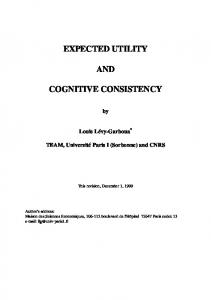
Figure 1 shows two density functions which satisfy the above conditions. Specific functions which will satisfy these conditions include the normal, double exponential, and triangular. Proof The function 11(y) has less weight in its tails than does h (y); so variate Y1 has a smaller variance than does Yz (Rothschild and Stiglitz). Since both variables are symmetric, the following inequality expresses the relationship between variances: (1)

2[(Y -

I

IJ-F fl(Y)

M+ d (y -

dy < 2[(Y - 1J-)2 hey) dy; or

IJ-F fl(Y)

dy

+ J'" (y - IJ-F fl(y) dy ~d

M

Proposition

J

< :+d (y - 1J-)2 h (y) dy + '" (y - 1J-)2 hey) dy ; In our work, we assumed that mean-variance analJ~d ysis (or QP) is a means of solving an expected and finally, utility problem. We argue elsewhere that for certain symmetrically distributed variables, the QP soluJ~d(y - 1J-)2 [(leY) - hey)] dy tion includes those activities with maximum expected utility for that mean value (Johnson and < Joc (y - 1J-)2[f2(Y) - fl(y)]dy. Boehlje l.? In other words, the set of activities with ~d the lowest variance (for a given mean) also has the highest expected utility. Likewise, the validity of Next, two nonnegative functions can be defined using alternate techniques should be based on how g(y) = .ft(y) - hey), JL < Y < JL + d; and well they approximate expected utility solutions, hey) = j;(y) - .ft(y), JL + d < y < 00. not QP solution variances. To that end, we propose the following: if (a) two variates Y1 and Yz are Since symmetric variables have one half their probsymmetrically distributed with the same means, ability in their right tail, the amount by which the and (b) density functions 11 (y) and h(y) are such probability mass ofIl(Y) exceedsfz(y) in the region that.ft(y) 2:fz(y) everywhere in the region JL - d < y JL < Y < JL + d is exactly offset by the amount by < JL + d (with strict inequality for at least one which fz (y) exceeds 11(y) in the region JL + d < interval in the region) and elsewhere fz(y) 2: .ft(y), y < 00, or then 11 (y) will have the smaller variance and also ll- +d g(y) dy = I'" the smaller MAD (mean absolute deviations). h(y) dy. (2)

IM

Donald Johnson is an economist with the Caterpillar Tractor Company; Michael Boehlje is a professor, Department of Economics, Iowa State University. Journal Paper No. 1-9954 of the Iowa Agricultural and Home Economics Experiment Station, Project No. 2064. 1 We used a RAND code which must solve in computer memory. Large models were costly to solve and, in one case, exceeded internal storage capacity. Also we were not able consistently to obtain feasible solutions until we changed default parameter specifications and tolerances. The default parameter values we used are available upon request. 2 This requires that density functions meet the conditions outlined in the proposition and that utility functions have derivatives which alternate in sign, beginning with a positive first derivative.

~d

The above regions can each be subdivided into n smaller regions (indexed by i) such that (3)

for i = 1, ... , n . For each of the regions of equal area, it is also true that (4)

L. (y I

1J-)2 gj(Y) dy