Minimizing Node Churn in Peer-to-Peer Streaming - Semantic Scholar

Minimizing Node Churn in Peer-to-Peer Streaming Constantinos Vassilakis∗ Greek Research & Technology Network, Athens, Greece

Ioannis Stavrakakis∗ Department of Informatics and Telecommunications, National and Kapodistrian University of Athens, Greece

Abstract Several Peer to Peer (P2P) streaming systems have proved by now their ability to deliver live video streams to hundreds of users. However the inherent instability of the distribution environment poses several obstacles for these systems to manage to deliver a high quality experience to the end users. In this paper we explore node churn which independently of the distribution topology adopted, is an “anomaly” to the operation of the system leading to the degradation of playout quality. We argue that node churn is service specific and that churn in a P2P streaming service is highly correlated to the quality experienced at each node. On this basis we contribute a novel churn model to capture this twofold relationship and reveal unknown till now interactions while operating popular peer selection strategies under node churn. We provide evidence that selection strategies aiming solely at either efficiency or stability of a connection, although efficient for other P2P services such as P2P file sharing, lead to the formation of distribution topologies that are highly sensitive to node churn resulting in degraded performance. We propose a peer selection strategy designed to be P2P streaming service specific that takes decisions in short time scales while balances several factors such as connection efficiency, connection stability and content availability. It is proved that this approach achieves a uniform development of the distribution topology and leads to superior performance in terms of both low node churn and increased experienced quality. Keywords: Node churn, peer to peer streaming, node churn model, peer selection strategies

1. Introduction Distributing a live video stream using a Peer to Peer (P2P) streaming system has the advantage over a point-to-point client/server system of offering more resources to clients by effectively turning each one of them into a secondary server that assists in the distribution of the stream. These additional resources yield improved scalability and/or resilience, depending on the design of the system. Node Churn: However, while the main advantage of P2P technology is this high availability of resources, its main drawback is that the distribution network is formed by highly transient peers who join and leave the system (churn) at their own will. This natural instability poses a major problem, especially in the case of P2P streaming where there are strict timing requirements for the delivery of content and an efficient and stable connection to the service is highly desirable. A peer leaving the system either permanently disconnects from the streaming service (node churn) or just leaves the current stream transmission and joins the transmission of another stream (change of channel, zapping, channel churn[1]) when other channels are offered by the service, as commonly are. Either cases have the same effect to the distribution of a specific ∗ Corresponding

author. Email addresses: [email protected] (Constantinos Vassilakis), [email protected] (Ioannis Stavrakakis)

Preprint submitted to Computer Communications

April 15, 2010

stream since the departing peer stops contributing with its resources to the delivery of a stream. In the following when we refer to node churn we refer to channel churn as well. Organizing the nodes into a tree, where the root is the source of the transmission, shoots for scalability while meshes on the other hand shoot for resilience to congestion/churn [2]. Mesh-like distribution [3, 4] attempts to conceal the environment’s instability from the end-user by providing several concurrent connections between peers (multiple-parent systems) providing this way higher reliability compared to treelike distribution [5, 6, 7, 8] (single-parent systems). However, even if multiple-parent systems ideally achieve to always retain some connection to the service, they do not always achieve to effectively retain service quality[9]. This owes to the fact that it is not always possible to have the required for playback chunks delivered on time, especially after the churn of a parent peer who was assigned to commit the delivery of a specific sequence of chunks. This may lead either to a disruption in playback continuity if a single description stream is transmitted or to the degradation of video quality if multiple description coding 1 is employed; in this case loosing a connection results in loosing one of the video descriptions/layers and thus a degraded video is displayed at the end user although playback continuity is sustained. Lifespan-based protocols: Several approaches address the problem of this given instability of the environment providing organizational protocols aiming at avoiding the effects of node churn to the performance. In [10, 11] the authors argue and demonstrate that taking into consideration the expected session times of peers (their lifespans) yield systems with performance characteristics more resilient to the natural instability of their environments. Through active probing of over half-a-million peers in a widely-deployed P2P file sharing system, the authors determined that the session times of peers can be well modeled by a Pareto distribution. In this context, the implication is that the expected remaining session time of a peer is directly proportional to the sessions current length, i.e. the peer’s age. According to [12] for all heavy-tailed distributions (e.g., Pareto, Weibull, and Cauchy) the expected remaining lifetime increases and becomes stochastically larger with age. In contrast, light-tailed distributions (e.g., uniform and Gaussian), exhibit expected residual lifetimes that are decreasing functions of age. Finally, for the exponential distribution, age does not affect residual lifetimes since it does not exhibit memory. Thus, the observation of heavy-tailed peer lifetimes forms the basis for the introduction of a new lifespan-based approach for organizational protocols which by taking into consideration the expected session times of peers may yield more resilient/stable systems. In [13] the authors attempt to minimize node churn in a closed group of peers by appropriately selecting the members of the group. Similarly in [14], first, stable nodes are distinguished from others in a P2P streaming system and then an architecture of two levels with stable and unstable nodes is created in order to improve system’s performance. These works also exploit a peer’s age to infer the stability of a peer, since they adopt Pareto distributed peer lifetimes. Node churn in P2P streaming: None of the presented works has considered of dealing apart from the effects of node churn, with its causes as well, attempting to minimize the phenomenon itself. Recent measurement studies have revealed that node churn in P2P streaming is fundamentally different from node churn in P2P file sharing. Contrary to the user behavior exhibited in a file sharing service, participating users in a streaming service are impatient and terminate their participation into the service either due to loss of interest or due to low observed performance [5, 15]. It is proved that node churn not only affects performance but it is also a function of performance in terms of service quality. The existence of this twofold relation between churn and service quality opens a new perspective to the problem. Node churn in P2P streaming is a phenomenon that exists independently of the service quality but grows with the degradation of the latter. We argue that more elaborate organizational protocols are required for a P2P streaming service that would take into account this observation and head for connection stability and efficiency at the same time. Our contribution: In this work we motivate towards this direction by exhibiting the performance advantages of such an approach. We introduce a churn model that captures the twofold relation between churn and quality without yielding for its accuracy but mainly for its ability to produce this kind of correlation. 1 A layered coding scheme in which each layer/description/substream is independently decodable and full stream quality amounts to obtaining all the layers.

2

However, this model produces a Weibull peers’ lifetime distribution which reaches an agreement with most recent measurement studies in P2P streaming systems [16] and also indicates that a peer’s age is an exploitable measure of stability. This approach is quite different from that followed in several performance evaluations since peer lifetimes are not considered known “a priori” but they are the result of a dynamic process where a peer’s probability to churn depends on the service quality that this peer experiences. At all times during the evaluation of peer selection strategies, the background churn process is governed by the introduced dynamic model which produces churn as a result of the achieved/experienced quality. First, we consider that ideally and unrealistically each peer has knowledge of the underlying churn process, having knowledge of every other peer’s churn probability which reflects that peer’s stability. We make this assumption in order to be able to explore the best a selection strategy can do towards improving overall performance and reach into safe results. Then we consider the realistic case where a peer’s stability is inferred/approximated by considering its age (lifespan, session time). In this context we study peer selection strategies under node churn towards improving the stability of the distribution system as well as the overall quality of experience. We claim that peer selection strategies should be service specific taking into account the distinct characteristics of a service. Thus, we introduce a new approach in designing peer selection strategies for P2P streaming systems considering that selection and optimization should be performed considering short time scales in contradiction to the long time scales considered in a P2P file sharing service. It is proved that such an approach is beneficial in highly dynamic environments due to node churn and network congestion and leads to a remarkable performance improvement. The explanation to this is quite simple. In a P2P file sharing service it is meaningful to achieve stability of a connection over time and a high average connection rate. A user requires from this service to be able to obtain the requested files within a reasonable time period. Thus, a high variability in connection rate does not have a negative effect if the average download rate is high enough to ensure the delivery of the requested files in relatively short time. However, in P2P streaming, although we are interested in the stability of the connection, we are also interested in achieving a high connection rate in shorter time scales and not on the average over connection time. The rate at which new frames become available to the client must be adequate to support continuous video playout. A congestion period which may not be concealed with the consumption of frames that already exist in the client’s playout buffer which keeps frames ahead of playback, is considered to have the same effects as those of a broken connection due to churn of the parent node that was supplying the client with new frames. Furthermore, we show that popular approaches in peer selection that shoot either for efficiency or stability of a connection, although appropriate for services like P2P file sharing, they are not appropriate for a P2P streaming system under node churn. The topology of the overlay network formed as a result of the selection strategy is crucial for the overall performance. Selection strategies aiming at efficiency tend to create long distribution chains while strategies aiming at stability tend to create hotspots. Both topologies are highly sensitive to node churn. On the contrary, a random selection strategy tends to achieve load balancing and uniformly expands the topology but since it doesn’t take into account either efficiency or stability exhibits a degraded performance as the dynamics of the environment increase. In our evaluation we consider a single tree distribution topology in order to exhibit the maximum damage from a wrong design approach. Our initial intuition suggests that our results also extend to the more resilient mesh-like distribution systems but admittedly this requires further exploration and proof. Based on our findings we come up with design directives and propose a new peer selection strategy. The latter performs in short time scales balancing at the same time connection efficiency and stability requirements while taking into account content availability. The result of this approach is to achieve distribution topologies less sensitive to node churn while giving performance gains in the entire spectrum of the underlying network conditions. The remainder of the article is structured as follows. In Sect. 2 we present the proposed churn model. In Sect. 3 we present the peer selection policies considered. The details of the system adopted to assist us towards evaluating the selection strategies under node churn are presented in 4. Several simulation scenarios on multiple metrics and control parameters are presented in Sect. 5. Finally, Sect. 6 concludes the article.

3

Table 1: Quality rating scheme

MOS 5 4 3 2 1

Quality Excellent Good Fair Poor Bad

Impairment Imperceptible Perceptible but not annoying Slightly annoying Annoying Very annoying

2. A model for node churn in P2P streaming In this section we introduce a novel churn model which attempts to capture the correlation between node churn and the experienced performance in terms of experienced quality. This model provides at all times, a rational assignment of the probability of a peer to depart from the system (churn probability) according to the quality experienced at that peer until the observation time. Considering discrete time, a bernoulli trial is performed at every time slot; at time t a peer vi leaves ˜ i (t) is the the system with probability PQ˜ i (t) or remains into the system with probability 1 − PQ˜ i (t) where Q ˜ i (t) captures the playback continuity estimated quality experienced at the peer by time t. Quality estimate Q experienced at a peer which is considered as the most important measure of quality in a P2P streaming ˜ i (t) at time t is calculated by appropriately filtering several past short term quality estimations, service. Q decided by a model as a function of lost and repeated frames, in order to capture a user’s memory of an event that fades as times goes by. PQ˜ i (t) is decided according to a proposed mapping of the estimated quality to churn probability which lets as capture several probable user behaviors. The model we introduce and adopt results in Weibull distributed peer lifetimes as measurement studies indicate and differs from the other introduced churn models in that peer lifetimes are not taken “a priori” according to a probabilistic distribution but may change according to the quality the distribution system manages to deliver. In the following of this section we briefly provide the necessary background knowledge while then we get ˜ t experienced at a peer until some time t and a model into the details of a model that estimates the quality Q that associates this estimate with a probability PQ˜ t for the peer to leave the system. Finally, we decide the probability distribution that peer lifetimes follow as a result of the adoption of the proposed churn model. 2.1. Background It is widely accepted that the most important measure of service quality of a streaming system is the continuity of video playback at the user hosts [17]. Video playback continuity is affected by either Discontinuity; experienced by a user by viewing a “frozen” frame for some time or Loss; experienced as a scene that suddenly jumps ahead in time, skipping some of the ongoing activity [18]. The pattern of impairments in playback continuity observed by a user are highly dependent on the adopted playout policy. We have shown in [18, 26] that a delay preserving playout policy targeted to always retain a constant offset between playback and encoding times (synchronized playout) results in lower discontinuity and loss since it manages to maintain a “positive correlation” between buffer contents among different peers and thus permit seamless handoffs. Although other known artifacts caused by packet loss are also extremely annoying to a viewer, it is considered that by now modern compression methods [19] have managed to satisfyingly address this problem by providing the means for effective error concealment under common packet error rates. Mean Opinion Score (MOS) [20] provides a numerical representation of the perceived quality of received media after compression and/or transmission. The MOS is expressed as a single number in the range 1 to 5, where 1 is the lowest perceived quality, and 5 is the highest perceived quality. The MOS is generated by averaging the results of a set of standard subjective tests where a number of viewers rate the video quality of test sequences presented to them according to the rating scheme presented in Table 1. Subjective quality assessment tests on the effect of degradations in video continuity [21, 22] on the user perceived quality have revealed some interesting properties: • MOS decreases with the increasing of the durations of distortions. 4

• MOS decreases logarithmically with the frame rate. • The perceptual impact of frame freeze and frame skip is highly content dependent. • One frame length distortion is unrecognizable for viewers. • Viewers prefer a scenario in which a single but long freeze event occurs to a scenario in which frequent short freezes occur. There have been several attempts to define an objective function to predict MOS and capture properties like the aforementioned without the need to reference the original content. In the majority of the presented works, MOS is approximated by a mathematical function which provides a good fit to the results of subjective tests. This approach has proved adequate to approximate a user’s MOS after viewing a short video sequence, but not to predict MOS after viewing long video sequences as well. In [23] the authors have come up with a list of observations regarding quality experienced after viewing long sequences: • The impression of past quality weakens through time time; this is also known as the recency effect. • A video section with high degradation in quality will strongly affect the overall quality. • The range of evaluation scores widens as the duration of evaluation increases. • MOS is on an ordinal scale and its values do not necessarily linearly represent the subject’s sensory impression. For example, the difference in the observers sensory magnitude between “imperceptible” and “perceptible, but not annoying” is assumed to be the same as that between “annoying” and “very annoying”. However, this is not necessarily the case [24]. Furthermore, several studies have shown that in order to estimate subjective quality of long sequences with variable over time quality such those provided by a video streaming service simply averaging qualities of short-term sequences is not adequate. In this work, in order to define an objective quality assessment procedure that suits a streaming environment and which will be appropriate for predicting long-term quality we adopt an already presented model for predicting short-term quality and then predict long-term quality by appropriately averaging several short-term qualities predicted in past short periods in order to capture the recency effect. 2.2. A model to estimate experienced quality In [25] a MOS prediction process flow is introduced. The authors conduct subjective quality assessments examining various impaired short-term video sequences of 240 frames. Impairments in playback continuity are the ones considered and the impaired short-term video sequences include several frozen frames or/and several lost frames. The contribution of that work is a function for predicting MOS with input the total number of dropped (lost) and repeated (frozen) frames;this function provides a good fit to the results coming from several subjective tests, as commonly practised. Let l be the total number of dropped frames, r the total number of repeated frames, f the number of frames used for the prediction, then the predicted value of MOS at time t, Q(t) is computed as follows: e=l+r 240 ·e eˆ = f Q(t) = −0.571 · ln (ˆ e) + 4.6836

(1)

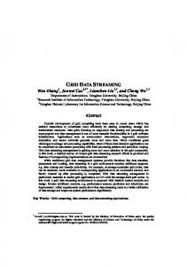
The authors provide evidence of the model accuracy for frame sequences of 240 frames but not for arbitrary long sequences of f frames (Fig. 1). We consider that for our purposes this model is adequate to capture the behavior-trend, not necessarily the exact mapping. We adopt this model for estimating quality experienced by a user after receiving a sequence of 240 frames over a time period τ . The experienced quality at some time is then estimated by computing an exponentially weighted average of a number of 5

5

Estimated MOS

4

3

2

1 1 10 20 30 40 50 60 70 80 90 100 110 120 130 140 150 160 170 180 190 200 210 220 230 240 Errors

Figure 1: Predicted MOS versus the sum of dropped and repeated frames for short video sequences of 240 frames (8

seconds)

qualities estimated in the past over continuous short term sequences. This way we are able to capture the recency effect which is considered as the most important feature when estimating quality experience after long viewing periods. Let Q(t) be the short-term MOS of the past τ -second interval at time t. Then the ˜ estimated overall quality of a long interval of T˜ seconds considered at time t, Q(t) is defined recursively by: ˜ = β · Q(t) + (1 − β) · Q(t ˜ − τ) Q(t)

(2)

where β ∈ (0, 1] is a weighting factor which when its more close to 1 gives more weight to most recent samples. 2.3. Mapping estimated quality to churn probability Although there is strong evidence that the probability of node churn is highly correlated with the quality the user experiences, the exact relationship is not yet known since this requires extensive measurement studies in deployed P2P streaming systems. The only clue we have is that 90% of users consider that a video streaming service is acceptable if a MOS above 3.5 is achieved [23]. In order to capture various probable behaviors we introduce an adaptive model which associates the ˜ with an increasing probability P ˜ for the peer to leave the system level of a client’s experience of quality Q Q and stop contributing to the service. We assume two given “boundary” probabilities P5 ,P1 (P5 > P1 ) for a user to leave the system when its estimated experienced quality level is 5 (best) and 1 (worst), respectively. Probability P5 captures the possibility a peer to leave the service for reasons other than dissatisfaction such as loss of interest. We also assume that all the other probabilities embed the probability for a peer to depart due to other reasons but it is considered that this is not the dominant one. We “spread” the difference between the ”boundary” probabilities P5 ,P1 over the distinct quality levels in between using an exponential function to implement various weights in this distribution. The probability

6

0.01

α=0 α=0.05 α=0.1 α=0.17 α=0.3 α=0.5 α=0.7 α=1 α=2

Churn Probability

0.008

0.006

0.004

0.002

0 1

1.5

2

2.5

3 Estimated Quality

3.5

4

4.5

5

Figure 2: Churn probability versus estimated quality according to the proposed mapping for P1 = 0.01, P5 = 0.00001 and various α values.

PQ˜ is given by:

˜

α

PQ˜ = P5 · ec·(5−Q) where µ ¶ P1 ln P5 c= 4α α≥0 ˜≤5 1≤Q 0 < P1 ≤ 1 0 < P5 ≤ 1 P5 ≥ P1

(3)

Parameter α shapes the distribution, letting us capture various user behaviors. In (Fig.2) we plot estimated quality versus churn probability according to our model for various α values. We take the case where P1 = 0.01 and P5 = 0.00001. α values which produce probabilities which exhibit an increase near a quality level close to 3.5 are considered to capture more closely the real case. 2.4. Peers lifetime distribution Adoption of the proposed model results in peer lifetimes with a probabilistic distribution which may be well approximated by a Weibull distribution. This implies that in a system evaluated under this model a peer’s age is an exploitable information providing an estimate of this peer’s remaining time into the system. In Appendix Appendix A we empirically show that the Weibull distribution provides a good fit to the distribution of peer lifetimes. However the shape of the distribution is system specific. 3. Peer selection strategies under node churn Latest mesh-like systems address connection reliability under node churn by maintaining several concurrent connections to other peers (multiple-parent systems) from which they download content in parallel. These systems exhibit a higher reliability compared to single-parent systems and perform better in unreliable environments. Although these systems manage to maintain a connection to the service at all times, there is always an associated cost for a peer loosing one of its active connections since this often leads to degradation of the received service quality. Thus, in both single-parent and multiple-parent systems; although in the first the effects are more severe, node churn is an “anomaly” in system’s operation affecting quality of playback. 7

Although different in the approach, most deployed P2P streaming systems base their peer selection strategies on whether a client peer may achieve a good network connection with a candidate parent peer which at the same time is able to provide the client peer with the required content. Recent proposals attempt to predict a peer’s stability in order to avoid the negative effects of churn. In [14] the authors identify the stable peers into a P2P streaming system and build a two-tier architecture of stable and unstable peers in order to improve the overall system performance. Their stability metric is based on the observation that the longer a peer stays in the overlay, the longer it is considered it would stay in the future; since it is found from measurement studies that peers lifetimes follow a probabilistic distribution that exhibits memory and heavy-tail like Pareto and Weibull and so a peer’s age gives us a clue about its expected remaining time into the system relatively to the other peers into the system. Ideally connections between peers in a P2P streaming system should be efficient and stable providing the required content at all times. Thus, a peer selection policy should take into account at the same time the: • connection efficiency; achievable data transfer rate • candidate peer’s stability • content availability; availability of requested frames and rate at which new frames become available We consider that the solution to the peer selection problem in a P2P streaming service is not obvious especially when taking into account node churn. We argue that in a P2P streaming system we should design our peer selection strategies considering short time scales. In a P2P file sharing service it is meaningful to achieve stability of a connection over time and a high average connection rate. However, in P2P streaming, although we are interested in the stability of the connection, we are also interested in achieving a high connection rate in shorter time scales and not on the average over the connection time. In the following we provide details on the selection strategies we consider, where we also propose new strategies embedding our observations under the operation of a churn process modeled by the churn model previously introduced. Initially, we consider policies assuming a peer’s churn probability as known while then we study ways of inferring a peer’s stability, which may not be obtained in a straight forward way, employing easily obtainable measures like a peer’s age. In order to avoid confusion, in a dynamic environment such the one considered, a peer’s stability reflects the probability for the peer to further remain in the system for long time while churn probability is its probability to churn at the time of examination. 3.1. Selection policies To perform peer selection a node vi is supplied with a random subset Vi ⊆ V : |Vi | = m ≤ n (n is the number of all peers in the system, V the set of all peers in the system) which includes those peers with whom vi may achieve an end to end connection rate adequate to support transmission at least at the stream’s nominal rate RN . We consider that all peers adopt the same delay preserving playout policy, Sync(D), according to which the time difference D between playout and encoding times is retained constant at all times; thus, all peers have synchronized playout points and playback the same video frame the same time. We have shown in [18, 26] the advantages of such an approach that creates a “positive” correlation of the playout buffer contents among different peers which in turn has as an effect the increased availability of peers which may supply another peer with the required frames when performing a parent change. Although we propose peer selection policies under synchronized playout among peers, these policies may be easily modified for other playout policies as well. Modeling the node churn process as described in the previous section, we consider three commonly used policies Random, BC and SO while we introduce a new policy named RVDO. Their description follows: 1. Random Connection (Random): According to the Random policy vi selects a parent peer vs ∈ Vi uniformly at random from Vi . 2. Best Connection (BC): Let Rij be the downstream estimated connection rate that peer vi may achieve with a peer vj . According to the BC policy vi selects that parent peer vs ∈ Vi with whom it may achieve the best connection rate; Ris > Rij ∀ vj ∈ Vi . 8

3. Stability Oracle (SO): Let Pj be the probability of peer vj to churn. As it is obvious, this information is not obtainable in reality since it assumes exact knowledge of the underlying churn mechanism. According to the (SO) policy vi selects that parent peer vs ∈ Vi with the minimum probability to churn among all the other peers in the provided set; Ps ≤ Pj ∀ vj ∈ Vi . 4. Reliable Volume Delivery Oracle (RVDO): Let bj be the number of frames ahead of playback in peer’s vj buffer. Let Pj be node’s vj churn probability at the time of selection. We want to compute the probability Pˆj for peer vj to remain in service and deliver a number of y frames to peer vi in order to select that peer with the highest probability to deliver the required frames. We assume that a time slot is equal to T which is the time taken for a frame to be delivered at the nominal stream rate RN (minimum rate required to support periodic playout). Thus, T is also the playout time of one frame or the frame period. We also assume that each candidate peer in Vi has one new frame available in its buffer every T or in other words that its connection with its parent peer is the minimum required to sustain its playback and equals to RN . So, a peer vj either has in its buffer the required y frames or will have them in the future at the rate of 1 new frame per time slot. It is obvious that we take the worst case scenario regarding the supply of node vj with new frames from its parent. This is true only in the case that the playout buffer is fully occupied and a new frame may be stored at every period T when the playout period of the frame currently presented at the user ends and thus the frame is discarded from the buffer leaving space for a new one. In the following we will further justify this choice. The estimated connection rate between vi and a peer vj is Rij ; thus, the time required for y frames to be delivered at this rate from vj to vi is xij time slots. Recall that Rij ≥ RN ∀ vj ∈ Vi . Then xij is given by: » ¼ y · RN xij = Rij It is clear that the maximum value for xij is y slots. However the required y frames may not be already in peer’s vj buffer and will be available in the future. The number of time slots required for the delivery of y frames is denoted by tij and given by: tij = max(xij , y − bj ) In the above formula, when y + bi − bj > 0 means that the required frames, all or some of them, are not available at node’s vj playout buffer and that they will be available in y + bi − bj time slots given that we have consider that one new frame is delivered every one time slot. If bi > bj then in order to have available the required y frames then vj must first receive in its buffer the bi − bj prior frames which are not yet available in its buffer. Since xij ≤ y then in every case tij = y + bi − bj . On the other hand, when y + bi − bj < 0 means that all y frames are available in node’s vj playout buffer, thus tij = xij . In any case the formula gives the actual time slots tij required for the node vi to get y frames given our assumption for the rate the parent node is supplied with new frames. Now we want to compute the probability Pˆj for the peer vj to remain into the system for as long as tij time slots in order to deliver the required frames. We deal with independent events and the decision for a peer to stay or leave is taken at every time slot. We consider that churn probability at the end of selection Pj remains the same for every time slot of the period tij . Then probability Pˆj is given by: Pˆj =

tij Y

(1 − Pj ) = (1 − Pj )tij

k=1

According to the RVDO policy vi selects that parent peer vs ∈ Vi with the maximum probability not to churn before it delivers y frames; Pˆs > Pˆj ∀ vj ∈ Vi . In the following we explore the behavior of the proposed policy and justify our choices. Deciding y: The choice of y affects the discrimination achieved among different Rij that candidate parent peers vj ∈ Vi may achieve with client peer vi . The highest recognizable by the algorithm value 9

for Rij is y · RN and all Rij values above this value are truncated to this. This is explained by the fact that a value Rij > y · RN means that y frames will be delivered in less than a time slot and xij = 1, according to its definition and in the case that the requested frames are available at the parent peer. Thus, a higher value of y results in a more fine grained discrimination of Rij . At the same time the choice of y affects the discrimination we may achieve among different buffer occupations bj among different candidate parent peers vj ∈ Vi . If a client peer with a small number of frames in its buffer requests also a small number of next frames (a low value for y), it is very possible to be able to find them in most of the candidate peers. The algorithm will not be able to recognize those candidate parent peers that have full buffers and benefit them in the selection process. The amount of frames a candidate parent peer has in its playout buffer indirectly reflects the average rate at which it is being supplied with new frames. A high occupation of the playout buffer indicates that the transmission rate from the source to this peer, over an overlay path that also passes through other peers, is good. This is desirable since we desire the client peer to be supplied with new frames at a high rate and not only achieve a high end-to-end transmission rate between parent and client peers. If the parent peer has no frames in its buffer to provide, even if the connection rate between parent and client peers is very high, then data transfer rate will be zero. To this point it is justified our choice to “punish” during the selection process those peers that do not possess the required frames by assuming that they are being supplied with new frames at a modest rate equal to the nominal stream rate RN . It is true that a peer with a full buffer receives new frames at a rate RN since a new frame may be stored in the buffer every T when a frame is displayed at a peer and then discarded leaving space for a new one. However this is not necessarily true for a peer with empty buffer space. Clearly our policy favors those candidate peers that may instantly provide more of the required frames to the client peer given that this may be supported by the transmission rate achieved between the client and candidate parent peers. This decision lies also on the tactic of taking short term decisions which are more appropriate for a service such as live video streaming. We have adopted the Sync(D) playout policy which enforces peers to have the same playout points. D Under this policy the highest occupation of a playout buffer equals D T , thus a value for y equal to T will allow the discrimination among all possible different buffer occupancies met at the candidate peers, even in the case that the client peer has an empty playout buffer. Adopting a higher value for y will not make a difference to the result of the selection process since the relative order of churn probabilities among the candidate peers will not be different to that when y = D T. Robustness: Indirectly the algorithm is able to recognize the rate at which a peer may be supplied with frames from a candidate parent peer and select the one that is most probable to deliver the requested frames given that the involved measures do not change during that delivery period. Considering that we seek for a compromise between efficiency and stability this policy exhibits robustness to the dynamically changing conditions of the environment. Having to decide among a set of peers with deviating stabilities (reflected by churn probability) and frame supplying rates (reflected by end-to-end connection rate and parent peer’s playout buffer occupation) then the selection will reflect this compromise. Considering now a case where candidate peers in the provided set exhibit more or less the same stability then the decision will lean towards the peer with the highest delivery rate. On the opposite if the peers in the set offer more or less the same delivery rates the peer with the highest stability will be selected. 3.1.1. Inferring a peer’s stability Since it is not possible to know the probability of a peer to churn we attempt to infer information about a peer’s stability from easily obtainable available information. The age of a peer is valuable information which may be easily provided by each peer and helps towards inferring its stability. The intuitive approach imposes that an older peer has a higher probability to have experienced a good quality of service since it has remained into the system for so long and thus it has a lower probability to churn. However, we can not infer any kind of information about a younger peer. The probabilistic approach imposes that a peer’s age is an exploitable information only if the peers lifetime distribution lacks the memorylesness property found only in the exponential distribution and furthermore this distribution 10

exhibits a heavy-tail as previously explained. Only in this case we may say that age is proportional to the remaining time of the peer in the system. Having an estimate Sˆi of a peer’s vi stability, expressed with a metric such as the age of the peer (the higher the age the higher the stability) we may not infer the peer’s probability to churn at a specific moment. Thus, for those proposed strategies (SO and RVDO) that deploy the “unknown” churn probability we must approximate their behavior by deploying only information that we may obtain. In the following we introduce Stability Prediction (SP) and Reliable Volume Delivery Prediction) (RVDP) strategies which approximate the behavior of SO and RVDO strategies respectively: 1. Stability Prediction (SP): According to the (SP) policy vi chooses that parent peer vs ∈ Vi with the highest stability estimate among all the peers in the given set, Sˆs ≥ Sˆj ∀ vj ∈ Vi . 2. Reliable Volume Delivery Prediction (RVDP): The same procedure followed in RVDO is also followed here until the computation of tij which is the number of time slots required for the delivery of y frames from a candidate peer vj to client peer vi given that a parent peer is fed with new frames with a rate equal to the stream’s nominal rate, RN . Then, k candidate peers with the lowest delivery times for the y frames are selected among the m peers in Vi (peers known to vi and used for the selection). According to RVDP, vi selects that parent peer vs ∈ Vi among all k candidates, with the highest stability estimate, Sˆs ≥ Sˆj ∀ vj ∈ Vi . Employing RVDP to select peers allows the equal selection of all peers including the “younger” peers; this is not true in the case where the only criterion employed for selection is a peer’s stability expressed by its age. When employing RVDP with the parameter k taking low values the behavior achieved is expected to be close to that of RVDO, while when parameter k takes high values then more stable peers (high age) will be selected and thus the behavior achieved will close to that of SO. For this reason in the following evaluation we neglect the study of SP since its behavior is that of RVDP when parameter k is taking high values. 4. System description In this section we present the details of the various components of the system considered in order to perform our evaluation. We start with the adopted playout policy and move on to the details of the single tree hierarchical P2P streaming system which we consider. Playout Policy: Let e(k) denote the encoding time for the kth frame and pi (k) be its scheduled playout time at node vi . Frames that become available at peer vi before their scheduled playout time are displayed at their exact playout time pi . Frames that miss their playout time are skipped. This amounts to synchronous playout between the source and node vi where by synchronous we indicate a fixed offset Di between encoding and playout times. That is: pi (k) = e(k) + Di . Let V be the set of all peers into the system. When Di = D, ∀vi ∈ V , all nodes display the same frame at the exact same time and a global synchronization is achieved. Initial Tree Build-Up: We assume that nodes form a single hierarchy rooted at the video source which transmits a single-description stream. A new peer vi selects a parent peer vj already in the system according to the illustrated peer selection strategy and connects to it (we discuss reconnecting peers and handoffs later). Node vi selects a specific frame from vj ’s playout buffer and starts prefetching it and all subsequent ones for a time interval Fij which leads to the desired offset Di between the playout of this first received frame at vi and its encoding time at the source. Details may be found in [26]. At the end of the prefetching period, the playout process starts. Performing Handoffs: We allow a node vi to be in either of the following two modes: Stable mode:A node is stably connected to its parent as long as its current buffer occupancy bi is above a threshold value Bh and its parent has not left the distribution tree. Handoff mode: A node enters a handoff mode as soon as its buffer occupancy falls beneath Bh or it is abandoned by its parent. The handoff amounts to selecting a new parent and connecting to it for a “grace 11

period” Tg before returning to stable mode. The grace period allows buffer build up thus avoiding cascading handoffs. Pre-active handoffs are employed to increase the chance for gap-free transitions when the connection to the current parent peer is not good enough, or when the latter has left the system. 5. Evaluation 5.1. Metrics We evaluate the peer selection strategies considered over the following metrics: Churn rate: It expresses the average rate with which peers leave the system. It is denoted by c and it is defined as the ratio of the number of peers that left the system during an examination period Tˆ to Tˆ. Churn rate also reflects the average peer lifetime since the lower the churn rate the higher the average peer lifetime. ¯ and it is defined as the average among all peers that entered the Average Quality: It is denoted by Q system during an examination period Tˆ of the average quality experienced at a peer during each lifetime into the system or until the end of Tˆ if it is still in at that time. 5.2. Description of the Simulation Model Initial tree formation: We assume discrete time with slot duration set equal to the frame period T . Peers enter the network according to a Poisson arrival process of rate µ arrivals/slot. Thus, during the examination period Tˆ on the average µ · Tˆ peers have joined the streaming hierarchy. Video source: The normal playback rate is set to 30 frames/sec, i.e., the video source at the root of 1 the delivery tree makes available a new frame every T = 30 seconds. Frame sizes are extracted from an educational video encoded in MPEG4 format at constant bit rate RN = 256 Kbps (LectureHQ-Reisslein trace file available at [27]). Native network topology and traffic model: Our model is based on the traffic model introduced in [28]. We adopt a native network topology which matches the core US topology of a large ISP (Sprint, AS 1239) estimated from the measurements of the Rocketfuel project [29], presented in Fig. B.11. The capacity of each intra-ISP link is chosen uniformly at random in the range [500,1500] Mbps. Peers of our system are assigned uniformly at random to the available access routers. The capacity of the link connecting a peer to an access router is considered asymmetric; the downlink capacity is uniformly distributed in [0.5,8] Mbps while the uplink capacity in [0.5,2] Mbps. According to the traffic model, traffic generating nodes assigned to a number of access routers generate traffic by initiating overlay flows between them according to a Poisson process with arrival rate Fα while the flow duration is exponentially distributed with mean Fd . Cross traffic is also modeled at each link. We control network load by altering the flow arrival rate Fa and traffic variability by altering flow duration Fd . In order to study our system under different loads we alter Fa while keeping Fd constant. In order to study our system under the same load but under different traffic variabilities we alter Fd while keeping Fa · Fd constant. The details of the model are available in Appendix Appendix B. 5.3. Experiments In the following we describe our simulation experiments and present our results. The default average number of peers that enters the system during simulation time is n = 1000, the 1 nominal rate of the stream is RN = 256 Kbps, the frame period is T = 30 seconds. All nodes use Di = D = 150 · T seconds, i.e., they pre-buffer up to 150 frames, which is also their buffer capacity Bc = 150. The buffer threshold for triggering a handoff is Bh = 10 frames , the grace period is Tg = 4 · Bh · T and the time between a disconnection and reconnection to a new parent peer is Th = 5 · T . Each simulation point in our results is the average of the outcomes of 30 independent runs each of which simulated 50000 time slots of system operation. In each graph the 95th -percentile confidence interval is drawn. 12

0.4

5 4.95 4.9 4.85

0.3

4.8 Quality

Churn rate (departures/sec)

0.35

0.25

4.75 4.7

0.2

4.65 4.6

Random BC SO RVDO(y=150)

0.15

0.1 20

40

60

80 Fa

100

120


4.55 4.5 140

20

40

60

(a)

80 Fa

100

120

140

(b)

0.24

5 4.98 4.96

0.2 4.94 Quality


0.22

0.18

4.92 4.9

0.16 4.88 RVDO(y=10) RVDO(y=50) RVDO(y=150) RVDO(y=300)

0.14

0.12 20

40

60

80 Fa

100

120

RVDO(y=10) RVDO(y=50) RVDO(y=150) RVDO(y=300)

4.86 4.84 140

(c)

20

40

60

80 Fa

100

120

140

(d)

Figure 3: (a) Churn rate versus Fa for Fd = 100, in the homogeneous case where each peer has full knowledge of other

peers in the system, for the policies Random, BC, SO and RVDO with parameter y = Bc = 150 (b) Average quality versus Fa and Fd = 100, in the homogeneous case where each peer has full knowledge of other peers in the system, for the policies Random, BC, SO and RVDO with parameter y = Bc = 150 (c) Churn rate versus Fa for Fd = 100, in the homogeneous case where each peer has full knowledge of other peers in the system, for the RVDO policy for different values of parameter y (d) Average quality versus Fa and Fd = 100, in the homogeneous case where each peer has full knowledge of other peers in the system, for the RVDO policy for different values of parameter y.

In the homogeneous case all peers into the system are considered to exhibit the same behavior. Same for all peers, in this case quality estimation is performed according to the proposed model with parameter β = 0.6 while churn probability is generated according to the proposed mapping with parameter α = 1. In the heterogeneous case each peer is considered to exhibit one out of three distinct behaviors considered. We consider patient, normal and impatient users while a peer’s behavior is selected uniformly at random among these three cases. Different behaviors are realized by adapting the α parameter accordingly to illustrate a user’s reluctancy to errors expressed by the associated churn probability. While we consider that for every peer quality estimation is performed according to the proposed model with parameter β = 0.6, for the patient peers we take α = 2, for the normal peers α = 1 and for the impatient peers α = 0.3. Experiment 1 (Homogeneous behavior, Global information): In this experiment we consider the homogeneous case where all peers exhibit the same behavior while each one of them has full knowledge of all other peers into the system. We operate the system for various network conditions by altering Fa (which expresses the network load) and Fd (which expresses variability). In Fig. 3(a) we plot churn rate versus Fa while in Fig. 3(b) we plot 13

0.3

4.9 4.88 4.86 4.84

0.26

4.82 Quality


0.28

0.24

4.8 4.78

0.22

4.76 4.74

0.2

4.72

Random RVDO(y=150)

0.18 200

250

300

Random RVDO(y=150)

4.7 350

200

250

300

Fa

350

Fa

(a)

(b)

Figure 4: (a) Churn rate versus Fa for Fd = 100, in the homogeneous case where each peer has full knowledge of

other peers in the system, for the policies Random and RVDO with parameter y = Bc = 150 (b) Average quality versus Fa and Fd = 100, in the homogeneous case where each peer has full knowledge of other peers in the system, for the policies Random and RVDO with parameter y = Bc = 150.

average quality versus Fa . In both cases we take Fd = 100 and present results for policies Random, BC, SO and RVDO with parameter y = Bc = 150. In this experiment Fa takes values within a range that produces a low average load (see Fig. B.10(a)). RVDO exhibits the lowest churn rate and the highest average quality throughout the whole range of Fa values. Next in performance comes Random, followed by SO while the worst performance is exhibited by BC. These performance differences become more clear in fig. 3(b) where average quality is drawn. Quality is kept in high levels for the studied loads, thus on the average churn probability is low according the adopted quality-churn probability mapping (see Fig. 2). As explained earlier,this mapping exhibits higher churn probabilities when quality falls under a value of 3.5, capturing this way presented experimental results, while changes in quality in the range of values higher than the value of 3.5 do not cause drastic changes in the associated churn probability. Taking a quick look at the results RVDO’s performance superiority is not the one that surprises us but rather the higher performance exhibited by Random compared to SO and BC. To explain this behavior we recall that in this experiment network conditions adopted are considered good while we have adopted Sync playout policy which ensures the high availability of peers to which a peer in handoff may find the required content. Thus, important role plays the rate at which a parent peer may provide content to a client peer. Given the good network condition at the core network, the uplink rate from the parent peer to the client peer highly depends on the parent’s available uplink bandwidth in conjunction with the client’s available downlink bandwith. Since we have adopted a single tree distribution topology, a parent’s available uplink bandwidth is the one that changes through time as it gradually serves more client peers. A client may be served by a parent with a minimum rate equal to the stream’s nominal rate and a maximum rate that equals the minimum between parent’s available uplink rate and client’s available downlink rate, given that required content is available for transfer at the parent’s peer buffer. According to BC policy the parent peer which may achieve the highest end-to-end transmission rate to the client at the time of selection is selected; without considering the existence or not of the required content at the parent peer. Consider an ideal case where each client’s available downlink rate is infinite or just greater than each peer’s uplink capacity (available uplink bandwidth when not serving anyone). Also, consider that all peers including the source of the transmission have the same uplink capacity. Given that each peer has full knowledge of other peers in the system and that peers join the system one after the other, performing peer selection with BC would result in this case considered to a distribution topology with the form of a chain from the source to the last peer that joined the system since during selection the candidate parent peer that serves none will always be best. In the realistic case where there is a variety of uplink and 14

0.4

5 4.95 4.9 4.85

0.3

4.8 Quality


0.35

0.25

4.75 4.7

Random(Fd=100) BC(Fd=100) SO(Fd=100) RVDO(Fd=100,y=150) BC(Fd=10) SO(Fd=10) RVDO(Fd=10,y=150) Random(Fd=10)

0.2

0.15

0.1 2000

4000

6000

8000 Fa*Fd

10000

12000

4.65 4.6 4.55 4.5 2000

14000

Random(Fd=100) BC(Fd=100) SO(Fd=100) RVDO(Fd=100,y=150) Random(Fd=10) BC(Fd=10) SO(Fd=10) RVDO(Fd=10,y=150) 4000

6000

(a)

8000 Fa*Fd

10000

12000

14000

10000

12000

14000

(b)

0.22

5

0.21

4.98 4.96

0.19 4.94

0.18 Quality


0.2

0.17 0.16

0.14 0.13 0.12 2000

4.9

Random(Fd=100) BC(Fd=100) SO(Fd=100) RVDO(Fd=100,y=150) BC(Fd=10) SO(Fd=10) RVDO(Fd=10,y=150) Random(Fd=10)

0.15

4000

6000

8000 Fa*Fd

10000

12000

4.92

4.88 4.86

14000

(c)

4.84 2000

Random(Fd=100) BC(Fd=100) SO(Fd=100) RVDO(Fd=100,y=150) Random(Fd=10) BC(Fd=10) SO(Fd=10) RVDO(Fd=10,y=150) 4000

6000

8000 Fa*Fd

(d)

Figure 5: (a) Churn rate versus Fa · Fd (expected number of flows creating load) for different values of Fd , in the

homogeneous case where each peer has full knowledge of other peers in the system, for the policies Random, BC, SO and RVDO with parameter y = Bc = 150, (b) Average quality versus Fa · Fd (expected number of flows creating load) for different values of Fd , in the homogeneous case where each peer has full knowledge of other peers in the system, for the policies Random, BC, SO and RVDO with parameter y = Bc = 150, (c) Churn rate versus Fa · Fd (expected number of flows creating load) for different values of Fd , in the homogeneous case with each peer having partial knowledge of other peers in the system (m=10), for the policies Random, BC, SO and RVDO with parameter y = Bc = 150, (d) Average quality versus Fa · Fd (expected number of flows creating load) for different values of Fd , in the homogeneous case with each peer having partial knowledge of other peers in the system (m=10), for the policies Random, BC, SO and RVDO with parameter y = Bc = 150.

15

downlink capacities in the system, performing peer selection with BC leads to a tree distribution topology with high tree depth. In such a topology, a congested overlay link or a peer’s churn close to the source would influence many other peers and possibly cause losses and as a consequence a change in their stability. According to SO policy the parent peer with the lowest churn probability at the time of selection is selected among all those candidate peers that may achieve an end-to-end transmission rate to the client at least equal to the stream’s nominal rate. Such an approach leads to a situation where many clients are served by those peers considered more stable. However, creating peers that serve many clients (hotspots) may prove bad when a hotspot is supplied through a congested link since this event will negatively influence many other peers served by this peer. At the same time, according to what we earlier mentioned, the transmission rate to each client goes down to the stream’s nominal rate as this parent peer serves more and more clients. A peer always served at the stream’s nominal rate has limited capability of refilling its buffer after recovering of a period of buffer drainage due to congestion and thus becomes more vulnerable to future congestion events. On the other hand, performing peer selection with Random policy benefits natural load balancing and the uniform development of the distribution tree having as a result not to create hotspots or long distribution chains which highly adds to performance. A similar topology is created as a result of adopting RVDO for peer selection. In addition, RVDO achieves higher performance since it manages to take into account at the same time during selection, content availability, transmission rate and peer stability. Performance gains when adopting RVDO become higher in comparison to adopting Random when the network load increases and thus a random selection becomes less adequate. This becomes clear in Fig. 4(a) and Fig. 4(b) where only RVDO and Random policies are compared for a range of values for Fa that produces high network load. In Fig. 3(c) we plot churn rate versus Fa while in Fig. 3(d) we plot average quality versus Fa . In both cases we take Fd = 100 and present results for the RVDO policy with different values of parameter y. RVDO’s performance increases as the value of parameter y increases up to the value of 150 which equals the maximum number of frames Bc that may be stored in a peer’s playout buffer, while for higher values for y performance remains almost the same. In other words RVDO exhibits its highest performance when y = 150. These results confirm our prior analysis, when introducing RVDO, on the effect of parameter y to the performance exhibited by RVDO. A value of y = 150 which equals playout buffer capacity Bc permits RVDO to be able to make a distinction between all possible buffer occupations of candidate peers, as well as to be able to make a distinction between different transmission rates among those candidate peers may achieve with the client. In Fig. 5(a) we plot churn rate versus Fa · Fd which is the expected number of flows creating load, for different values of Fd , for policies Random, BC, SO and RVDO with parameter y = 150. In Fig. 5(b) we plot average quality versus Fa · Fd for different values of Fd and for the same policies as before. Altering Fd while keeping the expected number of flows in the system constant, we are able to study the performance of different policies when average network load remains the same while variability changes. Recall that a lower value for Fd represents a higher variability. Although counterintuitive, we may observe in Fig. 5(a) and Fig. 5(b) that policies BC and SO exhibit a better performance in conditions of high variability for various network loads while policies Random and RVDO exhibit a slight decrease in performance. This may be explained by the fact that a higher variability triggers more often a parent change which in the cases of BC and SO works beneficiary since it increases randomness in selection, thus the creation of chains for BC and hotspots for SO is partially avoided. In the cases of Random and RVDO policies this phenomenon disrupts their normal operation and gets peers into the peer selection process more often. Experiment 2 (Homogeneous behavior, Partial information): We consider the case where each node has partial knowledge of other peers in the system, knowing at most a subset of m peers out of all peers in the system which are chosen for a client peer uniformly at random among those peers that may serve the client with a rate at least at the stream’s nominal rate RN . In this experiment all peers exhibit homogeneous behavior. In Fig. 6(a) we plot churn rate versus Fa while in Fig. 6(b) we plot average quality versus Fa . In both cases we take Fd = 100 considering that each peer is aware of m = 50 other peers in the system able to serve it. We present results for policies Random, BC, SO and RVDO with parameter y = Bc = 150. While for 16

0.28

5

0.26

0.22

4.9 Quality


4.95 0.24

0.2

4.85

0.18 0.16

4.8


0.14 0.12 20

40

60

80 Fa

100

120


4.75 140

20

40

60

(a)

80 Fa

100

120

140

(b)

0.22

5

0.21 4.98

0.19

4.96

0.18 Quality


0.2

0.17

4.94

0.16 4.92

0.15 0.14


0.13 0.12 20

40

60

80 Fa

100

120


4.9

4.88 140

(c)

20

40

60

80 Fa

100

120

140

(d)

Figure 6: (a) Churn rate versus Fa for Fd = 100, in the homogeneous case with each peer having partial knowledge of other peers in the system (m=50), for the policies Random, BC, SO and RVDO with parameter y = Bc = 150, (b) Average quality versus Fa and Fd = 100, in the homogeneous case with each peer having partial knowledge of other peers in the system (m=50), for the policies Random, BC, SO and RVDO with parameter y = Bc = 150, (c) Churn rate versus Fa for Fd = 100, in the homogeneous case with each peer having partial knowledge of other peers in the system (m=10), for the policies Random, BC, SO and RVDO with parameter y = Bc = 150, (d) Average quality versus Fa and Fd = 100, in the homogeneous case with each peer having partial knowledge of other peers in the system (m=10), for the policies Random, BC, SO and RVDO with parameter y = Bc = 150.

17

policies Random and RVDO performance seems unaffected by the fact that peer selection is performed over a subset of 50 peers, performance for BC and SO is better compared to the case where each peer performed peer selection over the set of all peers in the system. Performance exhibited by SO is very close to the one exhibited by Random. In Fig. 6(c) we plot churn rate versus Fa while in Fig. 6(d) we plot average quality versus Fa . In both cases we take Fd = 100 considering that each peer is now aware of only m = 10 other peers in the system able to serve it. We present results for policies Random, BC, SO and RVDO with parameter y = Bc = 150. Decreasing the number of other peers that a peer is aware of, to 10, we observe that performance for the policies BC and SO is further improved and becomes almost the same to that of Random policy. RVDO in any case sustains its superiority. Performance gains for BC and SO are well explained by the fact that as the number of other peers a peer is aware of, decreases, the randomness in peer selection increases making BC and SO operate more and more like the Random policy. On the other hand, Random and RVDO are unaffected by partial knowledge due to that network conditions considered are good on the average and due to that we have considered Sync as the adopted playout policy. In Fig. 5(c) we plot churn rate versus Fa · Fd for different values of Fd , considering that each peer is aware of m = 10 other peers in the system able to serve it, for policies Random, BC, SO and RVDO with parameter y = 150. In Fig. 5(d) we plot average quality versus Fa · Fd for different values of Fd , for the same case and policies as before. As it becomes more clear in Fig. 5(d) all policies are negatively affected in this case when variability is increased. This is easily explained by the fact that since BC and SO operate more or less as the Random policy illustrating increased randomness in selection, they are also negatively affected by the often parent changes triggered by the high variability. Experiment 3 (Heterogeneous behavior, Global information): In this experiment we consider the heterogeneous case where peers exhibit different behaviors drown from three distinct types considered; patient, normal and impatient. Each one of them has full knowledge of all other peers into the system. In Fig. 7(a) we plot churn rate versus Fa while in Fig. 7(b) we plot average quality versus Fa . In both cases we take Fd = 100 and present results for policies Random, BC, SO and RVDO with parameter y = Bc = 150. The performance observed for policies Random, RVDO and BC is slightly worse compared to that observed before in the respective homogeneous case. However, SO exhibits a severe performance drop which is now close to the one exhibited by BC. The decrease in performance for all policies is due to the fact that part of peers are “impatient” with an increased probability to churn. This has a higher effect on SO which tends to create hotspots; peers serving a high number of other peers, thus the effects of churn are higher than in the other policies. Experiment 4 (Heterogeneous behavior, Partial information):We consider the case where each node has partial knowledge of other peers in the system, knowing at most a subset of m peers out of all peers in the system which are chosen for a client peer uniformly at random among those peers that may serve the client with a rate at least at the stream’s nominal rate RN . In this experiment all peers exhibit heterogeneous behavior. In Fig. 7(c) we plot churn rate versus Fa while in Fig. 7(d) we plot average quality versus Fa . In both cases we take Fd = 100 considering that each peer is aware of m = 10 other peers in the system able to serve it. We present results for policies Random, BC, SO and RVDO with parameter y = Bc = 150. We observe that also in this case like in the respective homogeneous case BC and SO exhibit close performance to Random. However SO exhibits the worst performance for those reasons we already mentioned in experiment 3. Experiment 5 (The predictive policy RVDP): In this case we study the performance of the predictive policy RVDP when for the estimation of a peer’s stability we employ its age, in comparison with RVDO which ideally assumes knowledge of a peer’s probability to churn. In Fig. 8(a) we plot churn rate versus Fa for Fd = 100, in the homogeneous case where each peer has full knowledge of other peers in the system, for the policies RVDO with parameter y = Bc = 150, RVDP with parameters y = Bc = 150, k = 10 and RVDP with parameters y = Bc = 150, k = 50. In Fig. 8(b) we plot the average quality versus Fa for Fd = 100 for the same case and policies. RVDP and RVDO exhibit close performance when the value of parameter k is low, k = 10, while for higher values, k = 50, RVDP exhibits a worse performance. This owes to the fact that when we adopt a high value for parameter k selection is driven towards peers with the highest estimated stability and thus RVDP starts operating like SO policy 18

0.4

5 4.95 4.9 4.85

0.3

4.8 Quality


0.35

0.25

4.75 4.7

0.2

4.65 4.6


0.15

0.1 20

40

60

80 Fa

100

120


4.55 4.5 140

20

40

60

100

120

140

(b)

0.26

5

0.24

4.98

0.22

4.96

0.2

4.94

Quality


(a)

80 Fa

0.18 0.16

4.92 4.9


0.14 0.12 20

40

60

80 Fa

100

120


4.88 4.86 140

(c)

20

40

60

80 Fa

100

120

140

(d)

Figure 7: (a) Churn rate versus Fa for Fd = 100, in the heterogeneous case where each peer has full knowledge of

other peers in the system, for the policies Random, BC, SO and RVDO with parameter y = Bc = 150, (b) Average quality versus Fa and Fd = 100, in the heterogeneous case where each peer has full knowledge of other peers in the system, for the policies Random, BC, SO and RVDO with parameter y = Bc = 150, (c) Churn rate versus Fa for Fd = 100, in the heterogeneous case with each peer having partial knowledge of other peers in the system (m=10), for the policies Random, BC, SO and RVDO with parameter y = Bc = 150, (d) Average quality versus Fa and Fd = 100, in the heterogeneous case with each peer having partial knowledge of other peers in the system (m=10), for the policies Random, BC, SO and RVDO with parameter y = Bc = 150.

19

and adopting its disadvantages. On the contrary low values for k drive RVDP to exhibit close behavior to RVDO while all peers may be selected even those which are not much time in the system (“young” peers). Age reflects well a peer’s stability while the way we embed this measure in RVDP, results in performance gains which would be only possible if we could only know a peer’s probability to churn. In Fig. 8(c) we plot churn rate versus Fa for Fd = 100, in the homogeneous case with each peer having partial knowledge of other peers in the system (m=50), for the policies RVDO with parameter y = Bc = 150, RVDP with parameters y = Bc = 150, k = 10 and RVDP with parameters y = Bc = 150, k = 50. In Fig. 8(d) we plot the average quality versus Fa for Fd = 100 for the same case and policies. In this case also, we observe similar behavior as before. For k = 50 which equals to the number m of other peers that a peer is aware of, we may clearly observe a high performance drop due to the fact that in this case at each peer selection the peer with the highest estimated stability (age) is selected. Thus, selection policy resembles SO while “young” peers have very probability to be selected; this justifies the worse performance observed compared to SO’s performance in the respective case which we presented before. 5.4. Implementation issues As RVDO assumes full knowledge of the underlying churn process, it is not intended to be used in a real system but to assist our study in discovering the best it may be done when unrealistically there is knowledge of the underlying churn process. Clearly RVDO’s performance serves as an upper bound to the performance of the proposed deployable RVDP. Required information: The information required by RVDP when selecting parent peers may be easily drawn from them. What is required for each candidate in the selection set is each candidate parent peer’s buffer occupancy, connection time to the system (age) and the transmission rate that it may be achieved between the requesting client peer and each candidate parent peer. Buffer occupancy and age retrieval is straight forward while estimation of the transmission rate that may be achieved between the candidate parent peer and the requesting peer may be obtained quickly and with low error utilizing one of the several estimation methods available in the literature which are also implemented and are broadly available as tools. Scalability: Having in mind the scalability of the proposed methods every experiment in the evaluation has been conducted and results presented, not only for the case where the requesting peer has full knowledge of every other peer in the system but also for the case that each peer knows and makes its selection from a small subset of all the peers in the system. It has been proved that RVDP retains its performance advantaged also in this case of partial information and permits deployment of the method independently of the number of peers in the system. Communication cost: Furthermore, handoffs (selection and change of parent) are triggered only when the peer’s buffer occupancy falls below a certain threshold. This implies that a frequent communication between peers is not necessary. Also, when a handoff is triggered the peer seeking a new parent may support its playback for some time until its buffer is drained and this give some time to the selection process come up with a proposal for an appropriate new parent without having to produce instant results. 6. Concluding remarks In the following we summarize our key observations and findings while we provide directives for designing and evaluating peer selections strategies for P2P streaming under node churn: 1. Independently of the distribution topology adopted, node churn is an “anomaly” to the operation of the system, leading to the degradation of the playout quality. 2. Node churn is service specific. Node churn in P2P streaming is fundamentally different from node churn in P2P file sharing as proved by several measurement studies in the literature. Contrary to the user behavior exhibited in a file sharing service, participating users in a streaming service are impatient and terminate their participation into the service either due to loss of interest or due to low observed performance.

20

0.24

5 4.98 4.96 4.94

0.2

4.92 Quality


0.22

0.18

4.9 4.88 4.86

0.16

4.84 4.82

0.14 RVDO(y=150) RVDP(y=150,k=10) RVDP(y=150,k=50)

0.12 20

40

60

80 Fa

100

120

RVDO(y=150) RVDP(y=150,k=10) RVDP(y=150,k=50)

4.8 4.78 140

20

40

60

(a)

80 Fa

100

120

140

(b)

0.35

5 4.95 4.9 4.85

0.25 Quality


0.3

0.2

4.8 4.75 4.7

0.15 RVDO(y=150) RVDP(y=150,k=10) RVDP(y=150,k=50)

0.1 20

40

60

80 Fa

100

120

4.65

RVDO(y=150) RVDP(y=150,k=10) RVDP(y=150,k=50)

4.6 140

(c)

20

40

60

80 Fa

100

120

140

(d)

Figure 8: (a) Churn rate versus Fa for Fd = 100, in the homogeneous case where each peer has full knowledge of other

peers in the system, for the policies RVDO with parameter y = Bc = 150, RVDP with parameters y = Bc = 150, k = 10 and RVDP with parameters y = Bc = 150, k = 50, (b) Average quality versus Fa and Fd = 100, in the homogeneous case where each peer has full knowledge of other peers in the system, for the policies RVDO with parameter y = Bc = 150, RVDP with parameters y = Bc = 150, k = 10 and RVDP with parameters y = Bc = 150, k = 50, (c) Churn rate versus Fa for Fd = 100, in the homogeneous case with each peer having partial knowledge of other peers in the system (m=50), for the policies RVDO with parameter y = Bc = 150, RVDP with parameters y = Bc = 150, k = 10 and RVDP with parameters y = Bc = 150, k = 50, (d) Average quality versus Fa and Fd = 100, in the homogeneous case with each peer having partial knowledge of other peers in the system (m=50), for the policies RVDO with parameter y = Bc = 150, RVDP with parameters y = Bc = 150, k = 10 and RVDP with parameters y = Bc = 150, k = 50.

21

0.8

0.8

0.6

0.6 CDF

1

CDF

1

0.4

0.4

0.2

0.2

Avg loss ratio = 5% Weibull fit


0

0 0

5000

10000

15000

20000 Peer lifetime

25000

30000

35000

40000

0

5000

10000

15000

20000

25000

Peer lifetime

0.8

0.8

0.6

0.6 CDF

1

CDF

1

0.4

0.4

0.2

0.2



0

0 0

1000

2000

3000

4000 Peer lifetime

5000

6000

7000

8000

0

500

1000

1500

2000 2500 Peer lifetime

3000

3500

4000

4500

Figure A.9: Weibull CDF fit to various peer lifetimes CDFs produced operating the proposed model over a set of

independent peers under various average loss rates.

3. Churn and experienced quality are highly correlated. Churn in P2P streaming should be considered as the effect of how well system policies achieve to retain high quality and not as an independent phenomenon. Churn models should express this twofold relationship between churn and quality like the one we contributed in this work. 4. Peer selection strategies should be also service specific. Peer selection strategies for live video streaming should seek optimization in short time scales especially in highly dynamic environments. 5. Peer selection strategies for live video streaming should take into account at the same time content availability (availability at time of selection and rate at which new content becomes available), connection efficiency and candidate peer’s stability. 6. The distribution topology created as a result of the adopted peer selection strategy, is crucial for performance under node churn. Peer selection strategies should avoid creating churn sensitive distribution topologies; they should be targeted to achieve load balancing and uniform development of the topology while avoid creating long distribution chains and hotspots. 7. A peer’s age may provide a good measure of a peers stability since measurement studies show that peer lifetimes follow a heavy-tail distribution like the Weibull distribution. However this measure should be properly embedded in a peer selection strategy taking into account the above mentioned findings while avoiding the unbalanced selection between “elder” and “younger” peers. 8. The contributed RVDP strategy as a result of our study, smoothly embeds these findings and may be easily implemented. The approach it follows seems promising since it may provide superior performance compared to common approaches, in all network conditions and user behaviors. Appendix A. Peers lifetime distribution as a result of the adopted model: Empirical proof Considering discrete time, at each time slot t a bernoulli trial is performed for each peer who leaves the system with a probability PQ(t) or remains in it with probability 1−PQ(t) ˜ ˜ . It is known that binomial random 22

variables can be viewed as counting the number of successful outcomes in a series of independent bernoulli trials. It also known that the binomial distribution can be well approximated by the Poisson distribution when the number of trials is high and the probability of a successful outcome is small. This also stands for the case where the independent bernoulli trials are performed with different probability parameters [30] like here. In this case the parameter λ of the Poisson distribution which is the arrival rate of the successful outcomes (peer leaves the system) equals the sum of the probabilities at each trial as the number of trials tend to infinity. Recall that the probability at each trial depends on the estimated quality at that time. Since the rate parameter is not constant through time this is a non homogeneous Poisson process. In this special case of the Poisson process the waiting time until the first arrival/succesful outcome (peer leaves the system) is no longer exponentially distributed like in the homogeneous Poisson process. In the following, we empirically show that the Weibull distribution provides a good fit to the distribution of peer lifetimes. However the shape of the distribution is system specific. We leave the exact mathematical proof for future work. We assume independence in churn and permanent node failures. Consider 1000 peers coming into the system according to a Poisson process with arrival rate equal to 0.01. At every time slot each peer requires one frame for playback which is either available or lost. We model frame losses using a 2-state Markov chain (Gilbert model) with states 0 and 1 and transition probabilities p and q respectively. A peer remains in state 0 with probability 1 − p and transits to state 1 with probability p while a peer remains to state 1 with probabibility 1 − q and transits to state 0 with probability q. A peer in state 0 consumes the available frame while a peer in state 1 suffers from a frame loss independently of the others. According to the model the p average loss ratio equals to p+q and average burst length equals to 1q . The probability for a peer to stay or leave the system is decided at every slot, the churn probability is computed according to the proposed model with parameters α = 1 and β = 0.6 same for every peer. We consider an average burst length of 5 frames and various loss rates. We plot the CDF of the resulted peer lifetimes in Fig. A.9 and fit the results with the CDF of a Weibull distribution. Observe the very close fit as well as that for a low loss ratio it seems that the distribution takes the form of an exponential distribution. As loss ratio decreases estimated quality at every peer is almost the same, thus, all churn probabilities tend to a single probability value. Someone could come to the conclusion that a system running under this model would be more successful the more the resulted peer lifetimes distribution takes a close form to the exponential distribution; this would mean that the majority of peers leaves the system due to loss of interest and not to low observed performance and that system processes have managed to retain good quality at all peers. Appendix B. Details on the native network topology and traffic model adopted We adopt a native network topology which matches the core US topology of a large ISP (Sprint, AS 1239) estimated from the measurements of the Rocketfuel project [29], presented in Fig. B.11. The capacity of each intra-ISP link is chosen uniformly at random in the range [500,1500] Mbps. Routing is based on the shortest path algorithm and routes are considered to not change through time. Routers are either access routers or broadband routers. We consider 500 traffic generating nodes assigned to a number of access routers chosen uniformly at random. The capacity of the link connecting a traffic generating node and an access router is considered symmetric and taken uniformly at random within [8000,12000] Mbps in order to be able to create load at the core network without being restricted by bottlenecks created at the traffic generators’ connections to the core network. These nodes generate overlay flows between them. Overlay flows are generated according to a Poisson process with average arrival rate Fα and the flow duration is exponentially distributed with mean Fd . Thus, one may consider the system as an M/M/∞ queue where the expected number of active flows into the system is given by F1α . The origin and destination of flow are chosen according to a randomly Fd

generated (non-uniform) traffic matrix [31]. The maximum rate of a flow follows an exponential distribution with mean Fr . Cross traffic is also modeled at each native link as a fluid process with variable rate. The rate change events at a native link follow a Poisson process and the average time between a rate change event is Fc . 23

1 550

Fd=20 Fd=40 Fd=60 Fd=80 Fd=100

500

0.8

450

0.7

400

0.6

350 CDF

Average path throughput

Fa=100, Fd=5 Fa=25, Fd=20 Fa=6.25, Fd=80

0.9

300

0.5

250

0.4

200

0.3

150

0.2

100

0.1

50 20

40

60

80

100

120

140

160

180

0 -600

200

-400

-200

Fa

(a)

0 200 Available bandwidth changes

400

600

(b) 100

90

80

10

Percentage

Expected number of flows 10000 9000 8000 7000 6000 5000 4000 3000 2000 1000 0

70

60

20

30

40

50 Fa

60

70

80

90

100 0

100 90 80 70 60 50 Fd 40 30 20 10

50

40

Fd=20 Fd=40 Fd=60 Fd=80 Fd=100 20

40

60

80

100

120

140

160

180

200

Fa

(c)

(d)

Figure B.10: (a) Average path throughput versus Fa for various Fd values, (b) CDF of available bandwidth variations

in cases where the load is the same, (c) Expected number of active flows in the network versus Fa for various Fd values, (d) Percentage of paths with average path throughput greater than RN = 256Kbps versus Fa for various Fd values.

The rate of the cross traffic after a rate change event is chosen randomly as min(b, x · C), where b is the available bandwidth of the link, x is uniformly distributed in [0,1], and C is the link capacity. According to this model if a flow arrives on a saturated link then this flow will obtain zero throughput while it will not affect the other flows; thus, congestion control is not modeled. Network load is controlled by altering the flow arrival rate Fa and traffic variability by altering flow duration Fd or cross traffic average time between rate variations Fc . In our experiments we assume Fc constant and produce different loads and traffic variability by altering Fa and Fd . Shorter flows produce higher variability to the network. A pair of Fa and Fd values give a specific load and traffic variability. If we wish to retain the same load and just alter the variability we have to proportionally increase (decrease) Fa when increasing (decreasing) Fd so that the expected number of active flows into the network be the same; recall the M/M/∞ queue analogy. In Fig. B.10(c) the theoretical expected number of active flows is drawn against Fa and Fd . In Figs. B.10(a)(d) each simulation point drawn is the average of the outcomes of 10 independent runs each of which simulated 3000 seconds of system operation producing an average of measures taken every second. In Fig. B.10(a) we draw the average path throughput, reflecting the load of the network, which is the average throughput over all possible paths, versus Fa for various Fd values. It is clearly shown that load increases as Fa and Fd increase. In Fig. B.10(d) shows the average percentage of paths with available bandwidth higher than the nominal rate of a stream. For the same load as Fd decreases 24

Table B.2: Native network parameters

531 221 4052 [500,1500]Mbps

Number of traffic generators Traffic generator access link capacity

100 [8000,12000]Mbps

Peers downlink capacity Peers uplink capacity

[0.5,8]Mbps [0.5,2]Mbps

279

170

521 372

92 61

414 253

413

260 259

13 236

528 234

445

491

242

99

478

449

327

210

463

465 94

273

90

407

489

202 52

302

288 222

339

298

179

392

185

289

274

203

324

97

67 98

377 190

490

367 209

346

316

359

338

297

353 66

223 263

371 249

477

238 503

448

501

6 237

529

261

180 446

262

516

53 143 124

156

248

299 515

150

461

157

123

475

450

360

207

250

54

239

317

70

176

328

144 393

303

479

368

95

354

96

276

388

264

275

126

492

125 330

464 340

224

105 290

127 69

28

29 64

500

381 380

499

63

158

128

104

103

510 23

189 382

191

397

406

193

213

100 266

396 241

102 319

252

101

329

481

68

73 182

361

321

65

312

139 470 24

184 178

198 271

366

524 527

272

398

3 212

17 399

32

33 395

74

226 4

15

294 137

509

284

311 120 416

136

347

517

206

20 460

488 5

498 514

221

60

235 62

431 12 85

283

421 386

268

333 402

217 197

462

502

107

214

75 76

482 108

412

418 80

370

467

130

423

93

429

44

19 121 161

230 114

82 118

22 83

113 247

14 165

160 42

258

175 45

43 119 159 296 473

309

452

132

362 310

131 1 79 424

426 84 86 46

186

167

138

166

147 301

41 307

233 441

458

325

11

55

27

287 204

220 152

57 336

169 531

306

378

436 35 227 2 77

109

363 47

71 31

72

211 265 480

59 91 442

56 171

315

349

196

483

432

420

428 505

437

438

10

278 408

522

304

146

36

194

151

484

228

400 215 389

507 292

385

331

342

7

280

38

350

415 305

30

379

267

251

34

254

409

468

134

26

453

135

133

192 240 451 520 155 530 149

78

390

364

374

493

356

410 18 21

454 318 504

435 129

466 394

277 369

51 376 513

352

344 345

358

384

188 40

293

112 25 111

81 326

474

174 115

218

355

341

106

173 225

145

140

497

37

523 229

177

243 469

495

320

401

255

195

494

485

244

216 508

183

282

447 181

87

332 291

208

88 141 50

281

187

9 457

472 422

348 219

512 387

419

300 117

391 16

486

110

163

148

403

164

89

162

257

270

434

433

246

232

323

314

335

285

286

142

308

172

439 511

116 48

322

496

455 471

199 231

256 168

269

411

49 245

122 334

404

201

417

153

313

383 357 526

476

443 58

487 337

459

205

405

525

518

456

375

351 365

444

440

200

519

295 343

425

154 430 8

427

373

39

506

Number of routers Number of access routers Number of core links Intra-ISP link capacity

Figure B.11: Graphic representation of the core network topology considered in our simulation experiments.

the variability of the throughput increases and this is shown in Fig. B.10(b) where the CDF of the available bandwidth changes in a path from second to second at a single simulation run of 3000 seconds is drawn. Peers of our system are assigned uniformly at random to the available access routers. The capacity of the link connecting a peer to an access router is considered asymmetric; the downlink capacity is uniformly distributed in [0.5,8] Mbps while the uplink capacity in [0.5,2] Mbps. We assume discrete time and at every time slot equal to T 0 = 1 sec flows from the traffic generator nodes are served in a first come first served basis. After cross traffic takes bandwidth in each native link. Having created the network’s traffic, video streaming traffic generated by peers is transferred over the network. Each video streaming overlay flow between two peers utilizes the available bandwidth left by other traffic (flows and cross traffic) at the specific slot. In Table B.2 we present the native network parameters. [1] Z. Liu, C. Wu, B. Li, S. Zhao, Why are peers less stable in unpopular p2p streaming channels?, in: Networking, 2009, pp. 274–286. [2] N. Magharei, R. Rejaie, Y. Guo, Mesh or multiple-tree: A comparative study of live p2p streaming approaches, in: INFOCOM 2007, Anchorage, Alaska,6-12 May 2007. [3] X. Zhang, J. Liu, B. Li, T.-S. P. Yum, Donet/coolstreaming: A data-driven overlay network for peer-to-peer live media streaming, Vol. 3 of Proc. INFOCOM 2005, Miami, FL, USA, 13-17 March 2005, pp. pp. 2102–2111. [4] N. Magharei, R. Rejaie, Prime: Peer-to-peer receiver-driven mesh-based streaming, in: INFOCOM 2007, Anchorage, Alaska,6-12 May 2007. [5] S. Rao, Establishing the viability of end system multicast using a systems approach to protocol design, Carnegie Mellon University, Phd Thesis, Technical Report CMU-CS-04-168, Oct. 2004.

25

[6] H. Deshpande, M. Bawa, H. Garcia-Molina, Streaming live media over peer-to-peer network, Stanford University, Technical Report, 2001. [7] Y. hua Chu, S. G. Rao, S. Seshan, H. Zhang, A case for end system multicast, IEEE Journal on Selected Areas in Communication (JSAC), Special Issue on Networking Support for Multicast 20(8). [8] S. Banerjee, B. Bhattacharjee, C. Kommareddy, Scalable application layer multicast, in: ACM Sigcomm 2002, Pittsburgh, Pennsylvania, August 2002. [9] B. Li, S. Xie, G. Y. Keung, J. Liu, I. Stoica, H. Zhang, X. Zhang, An empirical study of the coolstreaming+ system, IEEE Journal on Selected Areas in Communications 25 (9) (2007) 1627–1639. [10] F. E. Bustamante, Y. Qiao, Friendships that last: peer lifespan and its role in p2p protocols, in: Web content caching and distribution: proceedings of the 8th international workshop, Kluwer Academic Publishers, Norwell, MA, USA, 2004, pp. 233–246. [11] F. E. Bustamante, Y. Qiao, Designing less-structured p2p systems for the expected high churn, IEEE/ACM Trans. Netw. 16 (3) (2008) 617–627. [12] Z. Yao, X. Wang, D. Leonard, D. Loguinov, Node isolation model and age-based neighbor selection in unstructured p2p networks, IEEE/ACM Trans. Netw. 17 (1) (2009) 144–157. [13] P. B. Godfrey, S. Shenker, I. Stoica, Minimizing churn in distributed systems, in: SIGCOMM ’06: Proceedings of the 2006 conference on Applications, technologies, architectures, and protocols for computer communications, ACM, New York, NY, USA, 2006, pp. 147–158. [14] F. Wang, J. Liu, Y. Xiong, Stable peers: Existence, importance, and application in peer-to-peer live video streaming, in: Proc. of INFOCOM 2008, 2008, pp. 1364–1372. [15] L. Vu, I. Gupta, J. Liang, K. Nahrstedt, Measurement and modeling a large-scale overlay for multimedia streaming, in: International Conference on Heterogeneous Networking for Quality, Reliability, Security and Robustness (QShine 2007), Vancouver, Canada, August 2007. [16] T. Silverston, O. Fourmaux, Measuring p2p iptv systems, in: ACM Network and Operating Systems Support for Digital Audio and Video (ACM NOSSDAV’07), June 2007. [17] X. Hei, Y. Liu, K. Ross, Inferring network-wide quality in p2p live streaming systems, IEEE Journal on Selected Areas in Communication (JSAC) 25(9) (December 2007) pp. 1640–1654. [18] C. Vassilakis, N. Laoutaris, I. Stavrakakis, The impact of playout policy on the performance of p2p live streaming...or how not to kill your p2p advantage, in: 15th Annual SPIE/ACM Multimedia Computing and Networking (MMCN ’08), San Jose, California, January 2008. [19] T. Wiegand, G. J. Sullivan, G. Bjontegaard, A. Luthra, Overview of the h.264/avc video coding standard, IEEE Transactions on Circuits and Systems for Video Technology 13(7) (July 2003) pp. 560–576. [20] I. T. Union, Methodology for the Subjective Assessment of the Quality of Television Pictures, ITU-R Recommendation BT.500-11, 2002. [21] Y. Qi, M. Dai, The effect of frame freezing and frame skipping on video quality, in: 2006 International Conference on Intelligent Information Hiding and Multimedia Signal Processing (IIH-MSP’06), Pasadena, California, Dec 2006. [22] Q. Huynh-Thu, M. Ghanbari, Impact of jitter and jerkiness on perceived video quality, in: Second International Workshop on Video Processing and Quality Metrics for Consumer Electronics (VPQM-06), Scottsdale, Arizona, Jan 2006. [23] H. T., K. G., O. J., T. A., Subjective quality estimation model for video streaming services with dynamic bit-rate control, IEICE Transactions on Communications 89(2) (2006) pp. 297–303. [24] S. Tasaka, Y. Ito, Psychometric analysis of the mutually compensatory property of multimedia qos, in: Proc. of ICC03, May 2008, p. pp. 18801886. [25] A. Younkin, R. Fernald, R. Doherty, E. Salskov, P. Corriveau, Predicting an average end-user’s experience of video playback, in: Third International Workshop on Video Processing and Quality Metrics for Consumer Electronics (VPQM07), Scottsdale, Arizona, 25-26 Jan 2007. [26] C. Vassilakis, N. Laoutaris, I. Stavrakakis, The impact of playout scheduling on the performance of peer-to-perr live streaming, Elsevier Computer Networks Special Issue on Content Distribution Infrastructures for Community Networks. [27] V. T. R. Group, http://trace.eas.asu.edu. [28] Y.Zhu, C. Dovrolis, M.Ammar, Dynamic overlay routing based on available bandwidth estimation: A simulation study, Computer Networks Journal 50(6) (April 13 2006) pp. 739–876. [29] N. Spring, R. Mahajan, D. Wetherall, T. Anderson, Measuring isp topologies with rocketfuel, IEEE/ACM Transactions on Networking 12(1). [30] R. Nelson, Probability, Stochastic Processes, and Queueing Theory: The Mathematics of Computer Performance Modeling, Springer Verlag, 2000. [31] A. Medina, N. Taft, K. Salamatian, S. Battacharya, C. Diot, Traffic matrix estimation: Existing techniques compared and new directions, in: Proc. of ACM SIGCOMM 2002, August 19-23, Pittsburgh.

26

Minimizing Node Churn in Peer-to-Peer Streaming - Semantic Scholar

Minimizing Node Churn in Peer-to-Peer Streaming - Semantic Scholar

Suggest Documents

Customer churn analysis - Semantic Scholar

Mobility Churn in DHTs - Semantic Scholar

Behavioral Modeling for Churn Prediction - Semantic Scholar

Computer Assisted Customer Churn Management - Semantic Scholar

Churn Models at Mobile Providers - Semantic Scholar

MINIMIZING OVERHEAD IN PARALLEL ... - Semantic Scholar

MINIMIZING DELAY IN LOSSLESS SEQUENTIAL ... - Semantic Scholar

Minimizing Makespan in Hybrid Flowshops - Semantic Scholar

Minimizing Unnecessary Handovers in a ... - Semantic Scholar

Minimizing incomplete automata - Semantic Scholar

Churn in Social Networks: A Discussion Boards ... - Semantic Scholar

Regular Register: an Implementation in a Churn ... - Semantic Scholar

Churn prediction in Telecom using Random Forest ... - Semantic Scholar

Caching in Opportunistic Networks with Churn - Semantic Scholar

Irregular Acoustic Streaming Formation in ... - Semantic Scholar

Streaming Media Distribution in VANETs - Semantic Scholar

compound media streaming in time - Semantic Scholar

node seniority ranking - Semantic Scholar

grid data streaming - Semantic Scholar

Minimizing Delivery Cost in Scalable Streaming Content ... - IEEE Xplore

Hardware/Software Partitioning and Minimizing ... - Semantic Scholar

Orthogonal Locality Minimizing Globality ... - Semantic Scholar

Minimizing Power Supply Noise Through ... - Semantic Scholar

Minimizing Hypoglycemia While Maintaining ... - Semantic Scholar