REVISTA INVESTIGACIÓN OPERACIONAL
VOL. 36 , NO 1. 85-95, 2015
MINIMUM POPULATION SEARCH – A SCALABLE METAHEURISTIC FOR MULTI-MODAL PROBLEMS Antonio Bolufé-Röhler*1 and Stephen Chen**2 *School of Mathematics and Computer Science, University of Havana, Cuba, **School of Information Technology, York University, Toronto, Canada ABSTRACT Minimum Population Search is a new metaheuristic specifically designed for optimization of multi-modal problems. Its core idea is to guarantee full coverage of the search space with the smallest possible population. A small population increases the chances of convergence and the efficient use of function evaluations, but it can also induce the risk of premature convergence. To control convergence and provide diversification, thresheld convergence is used as a main component of this new metaheuristic. Computational results show that Minimum Population Search performs competitively against Particle Swarm Optimization, Differential Evolution, and Univariate Marginal Distribution Algorithm on a broad range of multi-modal problems. KEY WORDS: heuristic search; population-based methods; multi-modal functions; thresheld convergence MSC: 90C59 RESUMEN Búsqueda de Población Mínima es una nueva metaheurística específicamente diseñada para la optimización de funciones multimodales. La idea fundamental consiste en garantizar la búsqueda en todas las dimensiones del espacio con la menor población necesaria. Una población pequeña aumenta las probabilidades de convergencia y el uso eficiente de las evaluaciones de la función objetivo, pero también aumenta el riesgo de una convergencia prematura. Para controlar la convergencia y promover la exploración la técnica de thresheld convergence constituye uno de los componentes fundamentales de esta metaheurística. Los resultados computacionales muestran que Búsqueda de Población Mínima es competitiva respecto a otros algoritmos en un amplio espectro de funciones multi-modales.
1. INTRODUCTION From basic geometry, two points define a line, three points define a plane, and n points define an n-1 dimensional hyperplane. If the population size (n) of an evolutionary algorithm is smaller than the dimensionality of the problem (d), then its population will define an n-1 dimensional hyperplane. New solutions generated strictly from the line segments formed among the population members (e.g. difference vectors, attraction vectors, mid-point crossover, etc) will “get trapped” inside this n-1 dimensional hyperplane which is a subset of the complete search space. This is an important consideration since line segments are a key aspect of many optimization techniques such as Nelder-Mead (NM) [12], Differential Evolution (DE) [18], and Particle Swarm Optimization (PSO) [3], [11]. In metaheuristics where the main search mechanisms are based on line segments, the population size needs to be larger than the dimensionality of the problem to avoid limiting search to an n-1 dimensional hyperplane. The Nelder-Mead algorithm is a clear example: a simplex of n = d+1 is required for a d-dimensional search space. In DE and PSO, the primary mechanisms of difference vectors and attraction vectors act within the n-1 dimensional hyperplane defined by the n population members. If population size is smaller than the 1
[email protected]
2
[email protected]
85
dimensionality of the problem (n < d), then secondary search mechanisms become responsible for generating new solutions outside the hyperplane. In PSO, the secondary mechanism is the “random vectors” of ε1 and ε2. In DE, it is the use of a crossover operator which acts on the axial dimensions as opposed to the population’s hyperplane. To guarantee the effectiveness of the difference/attraction vectors, the recommended population size for these metaheuristics is usually larger than the dimensionality of the problem [14]. However, large populations may affect a metaheuristic’s scalability and/or its ability to converge with a limited budget of function evaluations (FEs). Conversely, if the population is too small, then the metaheuristic may be prone to premature convergence and may even be unable to cover the entire search space (i.e. when n < d as is often the case for large d). Minimum Population Search (MPS) has been specifically designed to address this issue of scalability [2]. Using a population size equal to the dimensionality of the problem (n = d), new solutions are generated using difference vectors to be in a d-1 dimensional hyperplane. Full coverage of the search space is then achieved by taking a subsequent step that is orthogonal to this hyperplane. Calculating a vector orthogonal to two or three vectors is simple, but the computational cost increases rapidly for higher dimensions. Building up from the original design of MPS in two dimensions, this paper analyzes how to alleviate the costs associated with calculating the orthogonal step and still maintain an effective and methodical search into the full dimensionality of a problem’s search space while using a relatively small population. In the process, Minimum Population Search is formally defined and introduced as a new metaheuristic. The next two sections present a background on population-based heuristics and the initial development of Minimum Population Search. In Section 4, several options to extend MPS from two dimensions are analyzed. The design and implementation of the final, recommended version is described in Section 5, and computational results are presented in Section 6. A discussion about the new metaheuristic is carried out in Section 7 before the paper is summarized in Section 8. 2. BACKGROUND Population size is a fundamental parameter in the performance of population-based heuristics. Larger populations promote exploration, but they also allow fewer generations, and this can reduce the chance of convergence. Searching with a small population can increase the chances of convergence and the efficient use of function evaluations, but it can also induce the risk of premature convergence [14]. The optimum size may depend on several factors such as the characteristics of the objective function, the dimensionality of the search space, or the underlying search strategy. When optimizing multi-modal functions, metaheuristics can benefit from the increased exploration of larger populations which helps them escape/avoid local optima. As dimensions increase, it is also common to increase the population size in order to cover more regions of the search space. Whether the metaheuristic relies on statistical methods, recombination of building blocks, or difference vectors will also influence the optimal population size. The selection of the population size has been extensively addressed in the literature, and a brief review of the previous work reveals that there are many differing recommendations. For example, on typical problem dimensions (e.g. d = 1-100), a simple guideline for Differential Evolution is to use a population size that is ten times the dimensionality of the search space [17]. One of the most popular standards for Particle Swarm Optimization [3] uses a constant population size of n = 50. Estimation of Distribution Algorithms (EDA) usually require much larger populations of up to 2000 members [13]. If the risk of premature convergence can be avoided, then a population-based heuristic could benefit from the efficiency and faster convergence rate of a smaller population. To avoid premature convergence, it is important to have a diversified population. By including techniques for explicitly increasing diversity and exploration, it is possible to have smaller populations with less risk of premature convergence. In Estimation of Distribution Algorithms, explicit techniques for preserving diversity such as over-selection allow it to achieve good results with small populations (e.g. n = 50 for d = 100) [10]. For PSO, the use of dynamic neighborhoods, restarts, and mutation can lead to good results with a population as small as n = 5 [4]. In multi-swarm systems, which have an explicit/separate diversification mechanism, good results can be obtained with a swarm size of n = 15 [1]. In Minimum Population Search [2], this approach is extended to its limit in order to increase efficiency in the use of FEs. MPS can use the minimum population size of n = 2 members (for d = 2) – the use of one population member would make a metaheuristic indistinguishable from a point-search technique. Thresheld convergence (TC) is specifically used in MPS to preserve diversity and avoid premature convergence through
86
the establishment of a minimum search step [5], [15]. By disallowing new solutions which are too close to members of the current population, TC forces a strong exploration during the early stages of the search while preserving the diversity of the (small) population. The minimum step (threshold) decays as the search progresses and convergence is thus “held” back until the last stages of the search process. 3. MINIMUM POPULATION SEARCH FOR TWO DIMENSIONS In two dimensions, each iteration of MPS starts with the generation of “line points” along the subspace (line) determined by the two population members (x1 and x2). The “line points” are generated by adding the (normalized) difference vector formed by x1 and x2 to each population member xi (which acts as a parent once in each generation). The direction and size of the difference vector is determined by the scaling factor Fi (1),
linei = xi Fi ( x1 x 2 )
(1)
Taking a step along the line segment formed by x1 - x2 will only generate solutions in the subspace (line) defined by the two population members. An orthogonal step to this subspace (line) allows the search process of MPS to cover the full dimensionality of the (2D) problem. The direction and size of this exploratory step is determined by the Ostep_i factor (2). triali = linei Ostep _ i orth
(2)
Thresheld convergence forces new solutions to be a minimum (min_step) threshold distance away from the relevant parent solution(s). To ensure that the distance between a “line point” and its parent is smaller than the maximum allowed step (max_step), Fi is drawn with a uniform distribution from [-max_step, max_step] (note: the x1-x2 vector is normalized before scaling). To then ensure that the distance from the new trial solution (triali) to its parent solution (xi) stays within the [min_step, max_step] threshold range, the Ostep_i factor is selected with a uniform distribution from [min_orthi, max_orthi] (note: the orth vector is normalized before scaling). The min_orthi and max_orthi values are calculated by (3) and (4), respectively. Since the x1 - x2 vector is normalized before scaling, the Fi factor represents the actual distance between the “line point” (linei) and its corresponding parent solution (xi). New solutions which fall outside the feasible search space are clamped back to the boundaries. The two best solutions from the current population and the new trial solutions survive into the next generation. (3)
min _ orthi = max(min_ stepi 2 Fi 2 ,0)
(4)
max _ orthi = max(max_ stepi 2 Fi 2 ,0) The min_step and max_step values are updated by a rule similar to that used in previous attempts to control convergence for PSO [5] and DE [15] in which an initial threshold is selected that then decays over the course of the search process. Equation (5) shows how min_step is calculated (note: max_step = 2 * min_step). In (5), α represents a fraction of the main space diagonal, FEs is the total available number of function evaluations, k is the number of function evaluations used so far, and γ is the parameter that controls the decay rate of the threshold. The implementation presented in [2] uses α = 0.3 and γ = 3.
min _ stepi = diagonal ([ FEs k ] / FEs)
(5)
To ensure good spacing in the initial population, the initial points are selected to be on the diagonal of the search space. Assuming that the search space is bounded by the same lower and upper bound in each dimension (as in the used benchmark functions), the initial points are selected as x1 = (bound/2, bound/2) and x2 = (-bound/2, -bound/2). Figure 1 shows the search strategy of MPS in a two-dimensional search space.
87
Figure 1. Visualization of MPS search process in 2D.
4. EXTENDING TO HIGHER DIMENSIONS Minimum Population Search attempts to provide an efficient use of FEs by having a small population size. If the population size is smaller than the dimensionality of the search space, then the solutions generated through difference vectors will be constrained to the n-1 dimensional hyperplane. A smaller population size will lead to a more restricted subspace. With a population size equal to the dimensionality of the problem (n = d), the “line/hyperplane points” in MPS will be generated within a d-1 dimensional hyperplane. Taking a step orthogonal to this d-1 hyperplane will guarantee a complete search process that covers all the dimensions of the search space. The generation of “hyperplane points”, i.e. the solutions in the d-1 dimensional hyperplane, can be done by adding d-1 difference vectors to the parent solution (e.g. a difference vector between the parent and each of the other d-1 population members). A vector orthogonal to these d-1 difference vectors can then be used as the orthogonal step. A difficulty of this approach is obtaining the vector orthogonal to the d-1 dimensional hyperplane. This calculation has a high computational cost as it involves solving a system of linear equations (which often degenerates). To avoid this calculation, it is possible to simplify the algorithm. Instead of using all of the d-1 difference vectors, a subset of k difference vectors can be used to generate a “hyperplane point”. However, a low value for k causes information from only a small subset of the population to be taken into account. Conversely, larger values of k cause the cost of calculating the orthogonal vector to increase. Correctly tuning the value of k has proven to be a difficult task.
Figure 2. A comparison between using two difference vectors (left) and the centroid (right) for generating a new trial point in MPS.
88
Table 1. Comparison between orthogonal and centroid MPS for d=3 Function
MPS_O
MPS_C
Rastrigin Rotated
2.01e−1
8.13e−2
Weierstrass
1.89e−2
1.33e−3
Schaffers F7
2.07e−2
1.16e−5
Griewank-Rosenbrock
1.94e−2
9.64e−3
An alternative which avoids the parameter k is to use the centroid (xc) of the population. The population of MPS is the result of global elitist selection leading to the best solutions among parents and offspring. This strong selection means that the current members are representatives of the best search regions, and the centroid captures all of this information in a single point. In the centroid version of MPS, the “hyperplane points” are obtained by adding to the parent solution the difference vector between the parent and the centroid. The orthogonal step is done using a vector orthogonal to the parent-centroid line. This simplification has a low computational cost, uses information from the entire population, and avoids the parameter k. Figure 2 shows a graphical comparison in d = 3 between the MPS version using a vector orthogonal to the d-1 hyperplane and the centroid version. In the centroid version, the offspring solution (trial) can be on an entire plane (perpendicular to the centroid vector) as opposed to only a line that is perpendicular to the plane defined by x1, x2, and x3. The performance of both versions is compared in Table 1. As in the original MPS paper [2], results are presented for the Rastrigin Rotated, Weierstrass, Schaffers F7, and Composite GriewankRosenbrock functions (more details on these functions are given in Section 6). It can be seen that the centroid version leads to better results for all four functions.As dimensions increase, the use of a subset of k difference vectors (k < d) becomes necessary to keep running times low. To compare the effectiveness of using k difference vectors vs. the centroid version, an experiment was performed using the same four functions on different dimensions (d = 5, 10, and 20) – see Table 2. For each problem size, the parameter k was set to 1, 2, and 3. Results reveal that despite being conceptually and computationally simpler, the performance of the centroid version is generally superior to using k difference vectors. 5. MPS-CENTROID In two dimensions, the two population members were initialized on the search space diagonal. In higher dimensions, each population member is initialized using (6): sk is the kth population member, rsi are random numbers which can be -1 or 1, and bound is the lower and upper bound on each dimension. This initialization method leads to a better distribution of the initial solutions in the search space than did uniform random solutions. sk = (rsi * bound / 2, rs2 * bound / 2, ..., rsn * bound / 2) (6) At each generation, MPS-centroid (or simply MPS) performs a simple set of operations. First, the threshold values are updated (5) and the centroid is calculated. Then, each member is used as a parent solution to generate an offspring. The mechanism used to generate the new solutions is similar to the two-dimensional MPS, but the centroid is used instead of the other population member. The “hyperplane points” are obtained by adding the parent-centroid difference vector to the parent solution. The orthogonal step is made taking a Table 2. Comparison among different MPS versions d 5 10 20 d 5 10 20
MPS_1DV 4.18e+0 1.72e+1 4.70e+1
F15: Rastrigin Rotated MPS_2DV MPS_3DV 3.07e+0 3.46e+0 7.59e+0 7.29e+0 2.58e+1 2.77e+1
MPS_C 1.71e+0 4.58e+0 8.76e+0
MPS_1DV 1.34e−1 1.10e−1 7.66e−1
F16: Weierstrass MPS_2DV MPS_3DV 6.22e−2 2.37e−2 6.50e−2 5.89e−2 5.60e−1 4.17e−1
MPS_C 5.37e−1 5.71e−1 1.64e+0
d 5 10 20
MPS_1DV 4.78e−4 2.70e−2 2.18e−1
F17: Schaffers F7 MPS_2DV MPS_3DV 4.78e−4 4.78e−4 2.44e−3 7.48e−4 1.13e−2 1.45e−2
MPS_C 1.15e−5 1.54e−3 1.05e−2
F19: Composite Griewank−Rosenbrock d 5 10 20
89
MPS_1DV 1.67e−1 3.30e−1 1.79e+0
MPS_2DV 1.24e−1 2.85e−1 4.99e−1
MPS_3DV 1.61e−1 3.26e−1 5.33e−1
MPS_C 1.78e−1 2.30e−1 4.92e−1
Algorithm 1 Minimum Population Search MPS (α, γ, maxFEs) X ← InitialPopulation() while FEs < maxFEs min_step ← UpdateThreshold(α, γ) max_step ← min_step*2 xc ← CalculateCentroid() for i = 1 : popsize Fi ← UniformRandom(-max_step, max_step) orthi ← OrthogonalVector(xi- xc) orth_step ← UniformRandom(min_orth, max_orth) triali ← xi + Fi*(xi - xc) + orth_step*orthi endfor X ← BestSolutions(X, trial) endwhile
// Equation (6) // Equation (5)
// normalized vector // Equations (3) and (4) // clamping if necessary
random vector orthogonal (orth) to the parent-centroid difference vector. This two-step process for generating the new trial solutions (triali) is represented in (7). triali = xi Fi ( xi xc ) Ostep _ i orth
(7)
In (7), xi and xc are the parent and the centroid, respectively. The Fi factor is drawn with a uniform distribution from [-max_step, max_step] (xi-xc is normalized before scaling). The Ostep_i factor is selected with a uniform distribution from [min_orthi, max_orthi] (the orth vector is also normalized). The min_orthi and max_orthi values are calculated as in the two-dimensional version using (3) and (4). Once the new solutions are created, clamping is performed if necessary, and the best n solutions among the parents and offspring survive into the next generation. The parameters for the threshold function are α = 0.3 and γ = 3. A detailed pseudo-code is presented in Algorithm 1. 6. COMPUTATIONAL RESULTS A set of experiments has been designed to test the effectiveness of MPS. The experiments have been performed using the Black-Box Optimization Benchmark (BBOB) minimization functions [8]. There are 24 BBOB functions divided into five sets. Since MPS is explicitly designed for multi-modal search spaces, this paper focuses on Set 4-multi-modal functions with adequate global structure and Set 5-multi-modal functions with weak global structure. In Table 3, the names of these functions are given. The experiments include comparisons to other population-based metaheuristics with distinctive search strategies such as the Univariate Marginal Distribution Algorithm (UMDA), DE and PSO; as well as the simplex-based method Nelder-Mead. The UMDA algorithm is a standard implementation using Gaussian density functions and truncation selection [13]. PSO is a standard version with ring topology [3], zero initial velocities [7] and “Reflect-Z” for particles that exceed the boundaries of the search space [9]. The DE method is the highly common and frequently effective variant labeled DE/rand/1/bin [18]. The Nelder-Mead implementation is based on the fminsearch method in MATLAB. Table 3. BBOB functions Set
4
F
Function Name
Set
F
Function Name
15 16
Rastrigin, rotated
20
Schwefel
Weierstrass
21
Gallagher’s Gaussian 101-me Peaks
17
Schaffers F7
18
Schaffers F7, moderately ill-conditioned
22
Gallagher’s Gaussian 21-hi Peaks
23
Katsuura
19
Composite Griewank-Rosenbrock F8F2
24
Lunacek bi-Rastrigin
5
90
Table 4. Effect of population size n on performance for problems with d = 20 F15: Rastrigin Rotated n 100 80 60 40 20 10
UMDA 2.03e+1 2.08e+1 3.34e+1 4.48e+1 1.19e+2 2.95e+2
n 100 80 60 40 20 10
UMDA 2.14e+0 2.81e+0 2.87e+0 5.20e+0 9.52e+0 2.14e+1
DE 9.66e+1 9.29e+1 6.32e+1 2.96e+1 7.01e+1 2.28e+2
PSO NM 5.73e+1 5.27e+1 5.30e+1 5.23e+1 6.02e+1 3.11e+2 6.72e+1 F16: Weierstrass DE PSO NM 1.82e+1 5.37e+0 1.80e+1 5.49e+0 1.76e+1 6.22e+0 5.78e+0 6.71e+0 1.14e+1 6.91e+0 1.95e+1 1.02e+1 7.85e+0
F17: Schaffers F7 MPS 8.06e+0 7.69e+0 6.45e+0 6.05e+0 7.71e+0 1.41e+1
n 100 80 60 40 20 10
MPS 1.64e+0 1.56e+0 1.47e+0 1.36e+0 1.03e+0 1.39e+0
n 100 80 60 40 20 10
UMDA 1.04e−1 1.93e−1 3.88e−1 6.55e−1 2.73e+0 6.15e+0
DE PSO NM 1.94e−4 8.35e−1 5.98e−4 8.45e−1 3.67e−3 8.63e−1 4.08e−2 9.56e−1 1.01e+0 9.65e−1 2.10e+1 4.51e+0 1.71e+0 F19: Composite Griewank−Rosenbrock UMDA DE PSO NM 4.22e+0 3.83e+0 3.21e−1 3.89e−1 4.13e+0 3.73e+0 6.53e−1 4.10e+0 3.62e+0 1.08e+0 3.72e+0 3.78e+0 2.68e+0 3.90e+0 3.75e+0 7.40e+0 6.24e+0 4.46e+0 3.79e+0
MPS 5.31e−3 6.06e−3 4.61e−3 4.11e−3 2.70e−2 4.90e−2 MPS 4.20e−1 4.49e−1 4.26e−1 4.18e−1 4.17e−1 5.52e−1
6.1 Searching with small populations Population size is an important parameter in the performance of population-based metaheuristics. The population size is directly related to the efficient use of FEs, convergence rate, and exploration. Searching with smaller populations increases the efficiency, but it can also decrease exploration and induce the risk of premature convergence. In Table 4, the mean performance of several population-based metaheuristics (UMDA, DE, PSO, NM, and MPS) is presented using different population sizes (n = 100, 80, 60, 40, 20, and 10) for problems with d = 20 and a budget of 5000*d FEs. Among the 24 BBOB functions, F15 (Rastrigin Rotated), F16 (Weierstrass), F17 (Schaffers), and F19 (Composite Griewank-Rosenbrock) were selected to show the efficiency in performance vs. the size of the population. These functions are characterized as multi-modal, good global structure, and no ill-conditioning. It can be seen that the optimum population size is algorithm dependent. Based on statistical methods, UMDA has its best performance using the largest tested population size of n = 100. PSO and DE have their best performance on population sizes ranging from n = 40 to n = 100. In general, the performance of UMDA, DE, and PSO can vary greatly when their population sizes are changed. On the other hand, MPS appears to be much more robust to changes in population size. The use of thresheld convergence and the orthogonal step allow MPS to perform well with a population size as small as n = 10. From these results, the rest of the experiments in this paper use a population size of n = 100 for UMDA, n = 50 for PSO and DE, and n = d for MPS. 6.2 Optimizing Multi-modal Problems Results in [2] show that MPS performs well on multi-modal functions for d = 2 and d = 3. The new MPScentroid allows optimizing functions of any dimensionality. Tables 5 and 6 show the results of MPS for increasing dimensionality (d = 5, 10, 15, and 20) using all of the functions in BBOB Set 4 and 5 (multi-modal functions with and without adequate global structure). In Table 5, performance is measured with a reduced budget of function evaluations, i.e. FEs = 1000*d. Table 6 shows performance with the standard budget of FEs = 5000*d [8]. The results of MPS are compared against those of UMDA, DE, PSO, and NM. With a reduced budget of evaluations (i.e. FEs = 1000*d in Table 5), MPS performs best in 22 of 40 cases (passing a t-test with p < 0.05). In functions with adequate global structure (i.e. Set 4 in Tables 5 and 6), Minimum Population Search achieves the best performance in 26 of the 40 comparisons (passing a t-test with p < 0.05). In a multi-modal search space, following a gradient doesn’t necessarily lead the search in a good direction. An initial exploratory search is recommended to detect the most promising regions. Once these regions have been found, local search is required to converge to the corresponding (local) optima. The available function evaluations need to be efficiently used and distributed among these two processes of global and local search. The good performance of MPS on multi-modal functions is a direct consequence of it using the smallest population required to cover the full dimensionality of the search space. Using a small population allows performing more generations, and this increases the efficient use of FEs (especially with respect to convergence upon local optima).
91
Table 5. Performance as dimensions increase (FEs = 1000*d) d=5 Set
4
5
d =10 F 15 16 17 18 19 20 21 22 23 24
UMDA 2.39e+0 9.88e−1 7.08e−3 1.34e−1 3.12e−1 8.50e−1 1.68e+0 2.49e+0 1.29e+0 9.14e+0
DE 7.54e+0 2.64e+0 3.03e−3 1.69e−2 8.77e−1 7.50e−1 3.45e−1 4.61e−1 1.21e+0 1.33e+1
PSO 6.30e+0 7.63e−1 1.68e−1 5.88e−1 6.41e−1 6.18e−1 1.53e−1 1.84e−1 8.38e−1 1.15e+1
NM 5.52e+1 7.52e+0 1.05e+1 4.46e+1 3.00e+0 1.74e+0 1.30e+1 1.43e+1 1.13e+0 6.36e+1
MPS 2.27e+0 2.84e−1 1.75e−3 3.28e−2 3.48e−1 6.11e−1 1.13e+0 8.14e−1 2.29e−1 7.31e+0
UMDA 1.34e+1 1.40e+0 3.70e−2 4.91e−1 3.18e−1 1.79e+0 4.14e+0 4.70e+0 2.01e+0 3.86e+1
DE 6.94e+1 1.63e+1 1.76e−2 3.85e−1 4.00e+0 2.21e+0 3.26e+0 3.27e+0 2.08e+0 8.83e+1
PSO 6.02e+1 5.90e+0 1.01e+0 4.28e+0 3.64e+0 1.50e+0 9.50e−1 1.76e+0 1.49e+0 9.17e+1
NM 2.23e+2 1.38e+1 2.22e+1 1.01e+2 7.87e+0 1.75e+0 7.55e+0 1.56e+1 1.10e+0 3.43e+2
MPS 1.11e+1 1.27e+0 1.69e−2 3.53e−1 7.31e−1 1.49e+0 2.68e+0 4.49e+0 2.55e−1 2.53e+1
d = 15 Set
4
5
F 15 16 17 18 19 20 21 22 23 24
UMDA 8.25e+0 1.24e+0 4.49e−2 2.75e−1 6.77e−1 1.50e+0 2.66e+0 5.09e+0 1.73e+0 2.54e+1
DE 3.63e+1 1.07e+1 6.52e−3 1.07e−1 2.66e+0 1.78e+0 1.06e+0 2.30e+0 1.71e+0 4.51e+1
PSO 2.95e+1 2.78e+0 6.89e−1 2.40e+0 2.26e+0 1.26e+0 5.98e−1 1.43e+0 1.01e+0 4.38e+1
NM 1.28e+2 1.35e+1 1.71e+1 6.53e+1 4.73e+0 1.72e+0 2.00e+1 1.36e+1 9.02e−1 1.96e+2
MPS 6.67e+0 4.31e−1 1.17e−2 2.42e−1 5.03e−1 1.24e+0 3.08e+0 3.19e+0 2.75e−1 1.64e+1
DE 1.13e+2 2.07e+1 4.05e−2 8.63e−1 4.73e+0 2.24e+0 4.24e+0 3.81e+0 2.40e+0 1.30e+2
PSO 1.08e+2 8.13e+0 1.53e+0 6.21e+0 4.53e+0 1.88e+0 1.53e+0 1.45e+0 1.45e+0 1.49e+2
NM 3.15e+2 1.70e+1 2.79e+1 9.98e+1 8.19e+0 1.80e+0 1.33e+1 1.85e+1 1.09e+0 5.25e+2
MPS 1.38e+1 1.90e+0 3.02e−2 7.38e−1 9.69e−1 1.75e+0 7.30e+0 7.54e+0 2.74e−1 3.84e+1
d = 20 UMDA 1.51e+1 2.19e+0 1.09e−1 8.10e−1 4.25e−1 1.89e+0 7.54e+0 6.43e+0 1.20e+0 5.23e+1
Table 6. Performance as dimensions increase (FEs = 5000*d) d=5 Set
4
5
d =10 F 15 16 17 18 19 20 21 22 23 24
UMDA 1.75e+0 7.86e−1 1.12e−2 1.12e−1 1.82e−1 8.88e−1 1.33e+0 2.31e+0 6.92e−1 6.81e+0
DE 1.03e+0 2.02e−2 1.05e−4 6.44e−6 4.38e−1 5.69e−2 6.26e−1 4.66e−1 8.42e−1 8.66e+0
PSO 2.26e+0 8.01e−2 6.05e−3 7.68e−2 2.10e−1 2.35e−1 1.39e−1 8.38e−2 4.65e−1 7.15e+0
NM 3.55e+1 6.51e+0 1.24e+1 4.36e+1 4.37e+0 1.46e+0 7.44e+0 1.50e+1 1.14e+0 6.03e+1
MPS 1.71e+0 5.37e−1 1.15e−5 6.88e−3 1.78e−1 3.90e−1 1.32e+0 5.34e−1 1.56e−1 5.91e+0
UMDA 1.04e+1 1.37e+0 5.51e−2 5.02e−1 3.56e−1 1.67e+0 4.45e+0 5.62e+0 4.28e−1 3.10e+1
DE 1.33e+1 9.16e+0 2.76e−3 5.69e−2 3.20e+0 4.37e−1 1.90e+0 1.62e+0 1.63e+0 7.13e+1
PSO 3.17e+1 3.53e+0 4.94e−1 1.96e+0 2.77e+0 9.80e−1 6.93e−1 7.15e−1 1.05e+0 6.39e+1
NM 2.36e+2 1.34e+1 1.74e+1 7.79e+1 6.61e+0 1.70e+0 1.39e+1 2.25e+1 8.86e−1 3.51e+2
MPS 7.72e+0 9.18e−1 1.45e−3 4.31e−1 3.79e−1 1.25e+0 2.18e+0 4.13e+0 1.21e−1 1.88e+1
d = 15 Set
4
5
F 15 16 17 18 19 20 21 22 23 24
UMDA 6.92e+0 1.09e+0 2.93e−2 1.84e−1 3.99e−1 1.65e+0 2.49e+0 7.33e+0 4.84e−1 1.82e+1
DE 6.87e+0 2.50e+0 7.15e−4 4.84e−3 1.97e+0 2.05e−1 1.69e+0 3.28e+0 1.35e+0 3.37e+1
PSO 1.50e+1 1.18e+0 1.76e−1 7.18e−1 1.42e+0 6.92e−1 4.74e−1 8.04e−1 7.31e−1 3.01e+1
NM 1.10e+2 9.28e+0 1.61e+1 4.22e+1 5.88e+0 1.60e+0 1.76e+1 1.92e+1 8.42e−1 1.75e+2
MPS 4.58e+0 5.71e−1 1.54e−4 1.93e−1 3.30e−1 9.94e−1 1.41e+0 1.66e+0 1.56e−1 1.43e+1
DE 5.60e+1 5.84e+0 8.65e−1 3.40e+0 3.79e+0 1.10e+0 9.80e−1 1.99e+0 1.34e+0 1.16e+2
PSO 2.09e+1 1.81e+0 1.26e−1 6.18e−1 4.35e−1 1.93e+0 1.33e+0 1.49e+0 5.32e−1 5.73e+1
NM 3.11e+2 1.95e+1 2.10e+1 1.15e+2 7.40e+0 1.74e+0 1.36e+1 1.27e+1 1.03e+0 5.73e+2
MPS 7.71e+0 1.03e+0 2.70e−3 5.96e−1 4.17e−1 1.57e+0 3.44e+0 3.67e+0 1.19e−1 2.62e+1
d = 20
92
UMDA 2.03e+1 2.14e+1 1.04e−1 6.34e−1 3.21e−1 7.52e−1 3.27e+0 4.03e+0 2.07e+0 1.09e+2
6.3 Efficient Use of Function Evaluations The ability of MPS to effectively explore the search space with a small population allows performing more generations, and this increases the chances of convergence (of the population) with even a reduced budget of function evaluations. Figure 3 shows the performance of MPS on multi-modal functions as dimensions increase with a reduced budget, as well as a standard amount of FEs. The reported values are the relative performances (%-diff = (a-b)/max(a,b)) achieved by MPS versus DE, PSO, UMDA, and NM as dimensions increase. These values indicate by what amount (percent) the given algorithm (b) outperforms MPS (a), with negative values indicating that the competing algorithm has been outperformed by MPS. The result presented in Figure 3 is the average relative performance of all the functions in BBOB Sets 4 and 5. With a reduced budget of function evaluations, Minimum Population Search consistently outperforms the other metaheuristics. With a standard amount of FEs, MPS shows a steady increase in performance compared to PSO and DE as dimensions increase. In general, MPS does not only perform well on low dimensional problems, but its relative performance improves with dimensionality (from d = 5 up to d = 20).
Figure 3. Relative performance of DE, NM, PSO, and UMDA compared to MPS as dimensions increase for BBOB Sets 4 and 5.
7. DISCUSSION The key ideas behind the design of Minimum Population Search are the focus on multi-modal functions and to consider from the beginning the issues that may arise when scaling to large scale global optimization (LSGO) problems (i.e. d >= 1000). The problem with LSGO is that our intuitive understanding of metaheuristics often involves visualizations in two dimensions – for example, 15 to 30 birds searching in a cornfield [11]. However, a linear growth in population size (e.g. n = 10*d [17]) cannot maintain our visualized coverage as the search space grows exponentially. Going from d = 2 to d = 42 can increase the size of the search space by a factor of about 240 ≈ 1012. Whereas we might imagine 20 birds being able to fully explore a 10m x 10m courtyard, we should have a different visualization of 420 birds in an area similar to the size of the Atlantic Ocean. Since search space coverage will be sparse in high dimensions, we begin with the sparsest possible coverage that a population-based technique can have in two dimensions – i.e. n = 2 (because a population of n = 1 makes a technique indistinguishable from point search). Meaningful exploitation of the information available from these n = 2 population members is further complicated by the targeting of multi-modal functions (which creates a need for diversity) and the knowledge that two points define a line which does not provide full coverage of the 2D search space. The decisions to use thresheld convergence and the orthogonal step are based upon addressing these specific concerns (as we are also opposed to the proliferation of metaheuristics based upon questionable metaphors [16]).
93
Initial work using problems with d = 2 dimensions showed that MPS could outperform popular metaheuristics such as UMDA, DE, and PSO – especially with drastically reduced budgets of function evaluations [2]. Since search spaces increase exponentially with dimensionality and the allotted functions evaluations usually only increase linearly (e.g. [19]), we believe that the potential scalability of a metaheuristic can be better estimated by its performance in lower dimensions when function evaluations are highly restricted. For this reason, we have conducted experiments for both FEs = 1000*d and FEs = 5000*d in this paper. The generally superior performance of MPS compared to UMDA, DE, and PSO at both measurement points shows that the chosen search mechanisms for MPS hold the promise to be scalable across a broad range of problem sizes. Preliminary experiments show that MPS can perform better than DE and PSO all the way up to d = 200. However, none of these techniques performs exceptionally well on the LSGO benchmarks [19]. Going forward, we are in agreement with the suggestion that search techniques will need to focus more and more on gradient exploitation as dimensionality increases [6], so our primary focus is on hybrid techniques which will pair the full search space exploration performed initially by MPS with more efficient local search techniques. 8. CONCLUSIONS Building up from the original two-dimensional design, this paper formally defines Minimum Population Search as a new metaheuristic. MPS can effectively search a solution space with a relatively small population size, and this increases the chances of converging with even a limited budget of FEs. The use of thresheld convergence for balancing global and local search allows detecting the most promising regions during the early stages and performing an intensive/local search on those regions during the final stages of the search process. The combination of these two features leads to a high efficiency in the use of the available FEs. Overall, Minimum Population Search is shown to be a simple and effective algorithm for solving complex multi-modal problems. Future work will focus on hybridizing and adapting MPS for large scale global optimization. RECEIVED MARCH 2014 REVISED JULY 2014 REFERENCES [1] BOLUFÉ-RÖHLER, A. and CHEN, S. (2011): An analysis of sub-swarms in multi-swarm systems.
Australasian Conference on Artificial Intelligence, Perth. [2] BOLUFÉ-RÖHLER, A. and CHEN, S. (2013): Minimum population search – Lessons from building a
[3] [4]
[5] [6] [7] [8] [9] [10] [11] [12]
heuristic technique with two population members. IEEE Conference on Evolutionary Computation, Cancun. BRATTON, D. and KENNEDY, J. (2007): Defining a standard for particle swarm optimization. IEEE Swarm Intelligence Symposium. Honolulu. CABRERA-FUENTES, J. and COELLO, C. (2010): Micro-MOPSO: A multi-objective particle swarm optimizer that uses a very small population size. Multi-Objective Swarm Intelligent Systems, 1, 83104. CHEN, S. and MONTGOMERY, J. (2011): A simple strategy to maintain diversity and reduce crowding in particle swarm optimization. Australasian Conference on Artificial Intelligence, Perth. CHU, W., GAO, X., and SOROOSHIAN, S. (2011): A new evolutionary search strategy for global optimization of high-dimensional problems. Information Sciences, 22, 4909-4927. ENGELBRECHT, A. (2012): Particle swarm optimization: velocity initialization. IEEE Conference on Evolutionary Computation, Brisbane. HANSEN, N., FINCK, S., ROS, R., and AUGER, A. (2009): Real-Parameter Black-box Optimization Benchmarking 2009: Noiseless Functions Definitions. Technical Report RR-6829. INRIA. HELWIG, S., BRANKE, J., and MOSTAGHIM, S. (2013): Experimental Analysis of Bound Handling Techniques in Particle Swarm Optimization. Transactions in Evolutionary Computation, 17, 259-271. HONG, Y., KWONG, S., REN, Q., and WANG, X. (2007): Over-selection: An attempt to boost EDA under small population size. IEEE Conference on Evolutionary Computation, Singapore. J. KENNEDY and R. C. EBERHART. (1995): Particle swarm optimization. IEEE International Conference on Neural Networks, Perth. LAGARIAS, J. C., REEDS, J. A., WRIGHT, M. H., and WRIGHT, P. E. (1988): Convergence properties of the Nelder-Mead simplex method in low dimensions. SIAM Journal, 9, 112-147.
94
[13] LARRAÑAGA, P. and LOZANO, J. A. (2011): Estimation of Distribution Algorithms: A new Tool
for Evolutionary Computation. Kluwer Academic Publishers, Dordrecht. [14] MALLIPEDDI, R. and SUGANTHAN, P. N. (2008): Empirical study on the effect of population size on
differential evolution algorithm. Australasian Conference on Artificial Intelligence, Hong Kong. [15] MONTGOMERY, J. and CHEN, S. (2012): A simple strategy for maintaining diversity and reducing
crowding in differential evolution. IEEE Conference on Evolutionary Computation, Brisbane. [16] SÖRENSEN, K. (2013): Metaheuristics – the metaphor exposed. International Transactions in
Operation Research, 10. [17] STORN, R. (1996): On the usage of differential evolution for function optimization. IEEE Biennial
Conference of the North American Fuzzy Information Processing Society, Berkeley. [18] STORN, R. and PRICE, K. (1997): Differential evolution – A simple and efficient heuristic for global
optimization over continuous spaces. Journal of Global Optimization, 11, 341-359. [19] TANG, K., YAO, X., SUGANTHAN, P. N., MACNISH, C., CHEN, Y., CHEN, C., and YANG, Z.
(2007): Benchmark Functions for the CEC’2008 Special Session and Competition on High-Dimensional Real-Parameter Optimization. Technical report, USTC China.
95