Mining and Dynamic Simulation of Sub-Networks from Large Biomolecular Networks Xiaohua Hu1, Fang-Xiang Wu2, Michael Ng3 , Bahrad Sokhansanj4 1 College of Information Science & Technology, Drexel University, Philadelphia, PA 19104, Email:
[email protected] 2 Department of Mechanical Engineering, University of Saskatchewan, Saskatoon, SK S7N 5A9, Canada, Email:
[email protected] 3 Dept. of Mathematics, HongKong Baptist University, HongKong, Email:
[email protected] 4 School of Biomedical Engineering, Drexel University, Philadelphia, PA 19104 Abstract Biomolecular networks dynamically respond to stimuli and implement cellular function. Understanding these dynamic changes is the key challenge for cell biologists. As biomolecular networks grow in size and complexity, the computer simulation is an essential tool to understand biomolecular network models. This paper presents a novel method to mine, model and evaluate the regulatory system (a typical biomolecular network) which executes a cellular function. Our method consists of two steps. First, a novel scale-free network clustering approach is applied to the biomolecular network to obtain various sub-networks. Second, a computational model is generated for the sub-network and simulated to predict their behavior in the cellular context. We discuss and evaluate three advanced computational models: state-space model, probabilistic Boolean network model, and fuzzy logic model. Experimental results on time-series gene expression data for the human cell cycle indicate our approach is promising for sub-network mining and simulation from large biomolecular network.
1. Introduction We are in the era of holistic biology. Massive amounts of biological data await interpretation. This calls for formal modeling and computational methods. In this paper, we present a method to model the regulatory system which executes a cellular function, and can be represented as a biomolecular network. Understanding the biomolecular network implementing cellular function goes beyond the old dogma of “one gene; one function”: only through comprehensive system understanding can we predict the impact of genetic variation in the population, design effective disease therapeutics, and evaluate the potential sideeffects of therapies. As biomolecular networks grow in size and complexity, the model of a biomolecular network must
become more rigorous to keep track of all the components and their interactions, and in general this presents the need for computer simulation to manipulate and understand the biomolecular network model. However, a major challenge of modeling the dynamics of a biomolecular network is that conventional methods based on physical and chemical principles (such as systems of differential equations) require data that are difficult to accurately and consistently measure using either conventional or high-throughput technologies, which characteristically yield noisy, semi-quantitative, and often relative data. Therefore, there is a need to develop a computational model to incorporate the uncertainty. In this paper, we present a hybrid approach that combines data mining and advanced computational modeling to build and analyze the large biomolecular network of a cell process. Studying the community structure of biomolecular networks is of particular interest and challenging, given the enormous number of genes and proteins and the complex nature of interactions among them. In the context of biomolecular networks, subnetwork might represent structural or functional groupings, and can be synonymous with molecular modules, biochemical pathways, gene clusters, or protein complex. Due to the complexity and modularity of biomolecular network, another important reason is that it is more feasible computationally to model a biological meaningful sub-network containing a few dozens proteins which carry out certain cell functions. Our method consists of two steps. First, a novel scalefree network clustering approach is applied to the biomolecular network to obtain various sub-networks. The clustering algorithm considers the characteristics of the scale-free network graphs and is based on the local density of the vertex and its neighborhood functions that can be used to find more meaningful clusters with different density level. Second, a computational model is generated for the sub-network and simulated to predict their behavior in the cellular context. Three advanced computational models: state-space model,
probabilistic Boolean Network model, fuzzy logic model are used to predict the behavior of the subnetwork obtained in the first step. The rest of the paper is organized as follows: We describe a novel algorithm SNBuilder (Sub-Network Builder) in Section 2 for community structure analysis. The various computational modeling approach such as state-space model, probabilistic Boolean Network model, fuzzy logic model are discussed in Section 4 along with experimental results. Section 56 concludes with our main finding and future research directions. 2. Mining the Biomolecular Network to
Identify Sub-networks The interpretation of large-scale biomolecular network data depends on our ability to identify significant sub-structures (communities) in the data, a computationally intensive task. Many algorithms for detecting community structure in networks have been proposed. They can be roughly classified into two categories, divisive and agglomerative. The divisive approach takes the route of recursive removal of vertices (or edges) until the network is separated into its components or communities, whereas the agglomerative approach starts with isolated individual vertices and joins together small communities. One important algorithm is proposed by Girvan and Newman (the GN algorithm) [1]. The GN algorithm is based on the concept of betweenness, a quantitative measure of the number of shortest paths passing through a given vertex (or edge). The GN algorithm detects communities in a network by recursively removing these high betweenness vertices (or edges). It has produced good results and is well adopted by different authors in studying various networks [2]. However, it has a major disadvantage which is its computational cost. For sparse networks with n vertices, the GN algorithm is of O( n 3 ) time. Various alternative algorithms have been proposed [3,4], attempting to improve either the quality of the community structure or the computational efficiency. As discussed by [5], edge-betweenness uses properties calculated from the whole graph, allowing information from non-local features to be used in the clustering. Edge-betweenness algorithm does not scale well to larger graphs, this method is currently most appropriate for studies focused on specific areas of the proteome. The goal of our work here is to address a slightly different question about the community structure in a biomolecular network, i.e., what is the community to which a given protein (or proteins) belongs? We are motivated by two main factors. Firstly, due to the complexity and modularity of biological networks, it is
more feasible computationally to study a community containing a small number of proteins of interest. Secondly, sometimes the whole community structure of the network may not be our primary concern. Rather, we may be more interested in finding the community which contains a protein (or proteins) of interest. Our aim is to discover relatively small sub-networks such that proteins inside the sub-network interact significantly and, meanwhile, they are not strongly influenced by proteins outside the sub-network. Subnetworks are constructed starting with a seed consisting of one or more proteins believed to be participated in a viable sub-network. Functionalities and regulatory relationships among seed proteins may be partially known or they may simply be of interest. Given the seed, we iteratively adjoin new proteins following an adapted definition of a community in a network. The sub-networks built from our models may provide valuable theoretical guidance to experiment. In this study, we intuitively model the proteinprotein interaction network as an undirected graph, where vertices represent proteins and edges represent interactions between pairs of proteins. An undirected graph, G = (V, E), is comprised of two sets, vertices V and edges E. An edge e is defined as a pair of vertices (u, v) denoting the direct connection between vertices u and v. The graphs we use in this paper are undirected, unweighted, and simple – meaning no parallel edges. For a subgraph G’ ⊂ G and a vertex i belonging to G’, we define the in-community degree for vertex i, in
k i (G’), to be the number of edges connecting vertex i to other vertices belonging to G’ and the out-community out
degree, k i (G’), to be the number of edges connecting vertex i to other vertices that are in G but do not belong to G’. In our algorithm, we adopt the quantitative definitions of community defined by Radicchi and colleagues [6], i.e. the subgraph G’ is a community in a in
out
strong sense if k i (G’) > k i (G’) for each vertex i in G’ and in a weak sense if the sum of all degrees within G’ is greater than the sum of all degrees from G’ to the rest of the graph. The algorithm, called SNBuilder, accepts the seed protein s, gets the neighbors of s, finds the core of the community to build, and expands the core to find the eventual community. The two major components of SNBuilder are FindCore and ExpandCore. In fact, FindCore (line 8 to line 14) performs a naïve search for maximum clique from the neighborhood of the seed protein by recursively removing vertices with the lowest in-community degree until either 1) all vertices in the core set have the same in-community degree (Kmin = Kmax, i.e. the resulting subgraph is a clique); or 2) all
vertices except the seed have the same in-community degree (a star-like structure). The algorithm performs a breadth first expansion in the core expanding step. It first builds a candidate set containing the core and all vertices adjacent to each vertex in the core (line 16). A candidate vertex will then be added to the core if it meets one of the following conditions (line 21): 1) its in-community degree is greater than its out-community degree, i.e. the quantitative definition of community in a strong sense in
out
(k t > k t ); 2) its affinity coefficient is greater than or equals to the affinity threshold f. We define the affinity coefficient of a vertex to a network as the fraction of its in-community degree over the size of the network excluding the vertex itself in
(k t (D)/(|D|-1)). We introduce the affinity coefficient and the affinity threshold f to provide a degree of relaxation when expanding the core, because it is too strict requiring every expanding vertex to be a strong sense community member. Even though a candidate vertex may not have an in-community degree larger than out-community degree, it may connect to all (or even most of) other members of the network, indicating a strong tie between the candidate vertex and the network. We use an affinity threshold f of 1 in our implementation, meaning that in order to be eligible to add to the core set, the candidate vertex has to connect to all other vertices in the core set. However, f may be relaxed to be less than 1 if necessary or so desired. In addition, a distance parameter (d) is provided to restrict how far away a candidate vertex to the seed can be considered eligible for expansion. Quite often, a given seed may not always situate in the center of the resulting sub-network. The distance parameter serves as the shortest path threshold to ensure that all members of the obtained sub-network will be within specified proximity to the seed. A large enough value of d, such as one that is larger than the longest path from the seed to all other vertices in the network, will virtually lift this distance restriction. The FindCore is a heuristic search for a maximum complete subgraph in the neighborhood N of seed s. Let K be the size of N, then the worst-case running time of FindCore is O(K2). The ExpandCore part costs in worst-case approximately |V| + |E| + overhead. |V| accounts for the expanding of the core, at most all vertices in V, minus what are already in the core, would be included. |E| accounts for calculating the in- and outdegrees for the candidate vertices that are not in the core but in the neighborhood of the core. The overhead is caused by recalculating the in- and out-degrees of neighboring vertices every time the FindCore is recursively called. The number of these vertices is dependent on the size of the community we are building
and the connectivity of the community to the rest of the network, but not the overall size of the network. For biological networks, the graphs we deal with are mostly sparse and small world, therefore, the running time of our algorithm is close to linear. Algorithm 1 SNBuilder(G, s, f, d) 1: G(V, E) is the input graph with vertex set V and edge set E. 2: s is the seed vertex; f is the affinity threshold; d is the distance threshold. 3: N ← {Adjacency list of s } ∪ {s} 4: C ← FindCore(N) 5: C’ ← ExpandCore(C, f, d) 6: return C’ 7: FindCore(N) 8: for each v ∈ N in 9: calculate k (N) v
10 : 11 : 12 : 13 :
end for Kmin ← min { k v (N), v ∈ N} in
Kmax ← max { k v (N), v ∈ N} in
in
in
if Kmin = Kmax or (k i (N) = k j (N),
∀i, j ∈ N , i, j ≠ s, i ≠ j ) then return N
14 else return FindCore(N – {v}, k in (N) = K ) min v : 15: ExpandCore(C, f, d) 16 D ← ∪ {v, w} ( v , w )∈E ,v∈C , w∉C : 17 C’ ← C : 18 for each t ∈ D, t ∉ C, and distance(t, s) k t (D) or k t (D)/|D| > f then : C’ ← C’ ∪ {t} 22 end for : 23 if C’ = C then return C : 24 else return ExpandCore(C’, f, d) :
3. Computational Models for Simulation of Sub-Network and Results
Fig. 1. Comparison of experimental (solid lines) and predicted (dotted lines) gene expression profiles for DMFT(A), F2 (B), RRM2 (C) and TYR (D). Recently a wide variety of different computational models have been proposed for model biomolecular network. In this section we discuss and evaluate some of the advanced computational models, in particular, state-space model, probabilistic Boolean network model, and fuzzy logic model on high-throughput gene expression time series data for the human cell cycle [7].
3.1 Test Data Set To evaluate the accuracy and feasibility of computational approaches for biomolecular network modeling, we consider the gene network corresponding to a sub-network found using SNBuilder proposed in Section 2. This sub-network consists of 16 genes, and involves several important genes such as human genes related to p53, apoptosis, DNA damage response, and cell cycle. Edges in Figure 1 are taken to represent potential connections between genes, defining the structure of the gene network. In this paper, we employ the human cell cycle gene expression data [7] to construct the three computational models of the sub-network shown in Figure 1. There are independent data in [7] for five methods of cell cycle synchronization, two of which are complete for the genes in the sub-network we studied. One data set (“Thy-Thy 3”) is used as the “training set” to identify the parameters in model. A different dataset (“ThyNoc”) is used as the “testing set”.
3.2 State-space Model The state-space model for a gene regulatory network is mathematically described as [8]:
⎧ z (t + 1) = A ⋅ z (t ) + Bu(t ) + n1 (t ) ⎨ ⎩ x (t ) = C ⋅ z (t ) + n 2 (t )
(1)
where the vector x (t ) = [ x1 (t ) L xn (t )]T consists of the observation variables of the system and xi (t ) (i = 1, L , n) represents the expression level of gene i at time point t , where n is the number of genes in the network. The vector z (t ) = [ z1 (t ) L z p (t )]T consists of the internal state variables of the system and z i (t ) (i = 1, L , p ) represents the expression value of internal element (variable) i at time point t which directly regulates gene expression, where p is the number of the internal state variables. The vector u(t ) = [u1 (t ) L u r (t )]T represents the external input (control variable) of the internal state governing equation. The matrix A = [a ij ] p× p is the time translation
matrix of the internal state variables or the state transition matrix. It provides key information on the influences of the internal variables on each other. The matrix B = [bik ] p× r is the control matrix. The entries of the matrix reflect the strength of a control variable to an internal variable. The matrix C = [cik ]n× p is the
observation matrix which transfers the information from the internal state variables to the observation variables. The entries of the matrix encode information on the influences of the internal regulatory elements on the genes. Finally, the vectors n1 (t ) and n 2 (t ) stand for system noise and observation noise. In model (1) the upper equation is called the internal state governing equation while the lower one is called the observation equation.
1 Expression level
Expression level
1
0.5
0
0.5
0 B
A -0.5
0
5
10 Time
15
-0.5
20
5
10 Time
15
0.5
0
0
5
10 Time
15
0.5
0 D
C -0.5
20
1 Expression level
Expression level
1
0
0
5
10 Time
15
20
-0.5
20
Fig. 2. Comparison of experimental (solid lines) and predicted (dotted lines) gene expression profiles for DMFT(A), F2 (B), RRM2 (C) and TYR (D).
Let X be the gene expression data matrix with n rows and m columns, where n and m are the numbers of the genes and the measuring time points, respectively. The constructing of model (1) using microarray gene expression data X may be divided into three phases. Phase one identifies the internal state variables and their expression matrix, and estimates the elements of observation matrix C; Phase two, determine the control matrix B based on observation matrix C and the structure of the network; and Phase three estimates the elements of matrices A. Applying the state-space modeling method [8] to gene expression data of 16 genes in Figure 1, we obtained an inferred gene regulatory network with nine internal variables. In this study, the inferred networks will be evaluated in the following aspects: the prediction power, stability, robustness, and periodicity. To inspect stability, robustness, and periodicity of the inferred gene networks, the eigenvalues of the state transition matrices A are calculated. The eigenvalues of matrix follow as: -0.0715, 0.2479, 0.9018, 0.6749 ± 0.3959i, 0.8125 ± 0.2924i, 1.0396 ± 0.1536i. All eigenvalues except for the last pair of matrix A lie inside the unit circle in the complex plane, and the last pair is very closed to the boundary of the unit circle. This means that the inferred network is almost stable and robust. Furthermore, the dominant eigenvalues of the inferred network are pairs of conjugate complex number: 1.0396 ± 0.1536i. Accordingly, this implies that the network behaves periodically. This result is because the networks are inferred from cell-cycle regulated gene expression data. We also use the constructed model to predict the expression profiles from the testing dataset “Thy-Noc”. Figure 2 shows comparison of experimental and
predicted expression profiles of the four genes as in the training dataset. From Figure 2, agreement of the tendency of the experimental and predicted profiles is excellent for the testing dataset.
3.3 Fuzzy Logic Model The fuzzy biomolecular network model is a set of rule sets for each node (in this case gene) in the network governing the response to each fuzzy state of the input genes to that node (the output gene). The result for each input gene is summed to give the overall behavior of the output gene, resulting in a linear fuzzy model that has been called the “union rule configuration” (URC). URC fuzzy logic has been applied previously to modeling biological systems such as the lac operon of E. coli [9]. Fuzzy rule sets are generated for genes in the subnetwork in Figure1. Edges in Figure 1 are taken to represent potential connections between genes, defining the set of possible inputs to each gene. We generate all possible rule combinations for the inputs on each gene (including the “null” rule, equivalent to excluding a potential rule) assuming that if an expression level of an input gene is MEDIUM it must result in an output expression level of MEDIUM also. An example of a possible rule is “If Input is LOW then Output is LOW, if Input is MED then Output is MED, if Input is HIGH then Output is MED”). This is the same kind of exhaustive combinatorial rule search described in our previous work [10] contains the details of the method and an example of the implementation) but with fewer allowed rules and restricting the possible input genes to those identified by mining literature and clustering the resulting biomolecular network map. Three fuzzy sets are used to retain tractability of the rule search method,
0.6 0.4 0.2 0 -0.2 -0.4 -0.6 0
10
20
30
40
Log(Expression Ratio)
Log(Expression Ratio)
A
0.8
B
0.8 0.6 0.4 0.2 0 -0.2 -0.4 -0.6 -0.8 0
10
20
0.6
C
0.4 0.2 0 -0.2 -0.4 -0.6 0
10
20
30
40
30
40
Time Log(Expression Ratio)
Log(Expression Ratio)
Time
30
40
D
1 0.5 0 -0.5 -1 -1.5 0
10
20
Time
Time
Fig. 3 Best fit rule on training set “Thy-Thy 3” (as shown in Table 2) predicting gene expression on the test data set (solid line) compared to actual data from the test set “Thy-Noc” (dashed line) for CDK2 (A), BRCA1 (B), EP300 (C), and CDK4 (D).
which examines all potential hypotheses consistent with the data. However, this still represents a significant advance in resolution over Boolean logic, because of the non-binary membership in LOW and HIGH fuzzy sets. We again apply the resulting fuzzy rules to microarray gene expression time series data for the human cell cycle [7]. The data set (“Thy-Thy 3”) was used as the “training set”, and for each gene, exhaustively generated rule sets were ranked based on the error (E) of that rule set on the data. The rules were then simulated at each time point in the “test set”, a different kind of cell cycle synchronization (“ThyNoc”); As shown in Figure 3, agreement between the predictions of the best fit rule on the training set and the data in the test set is excellent in some cases, in particular CDK2 and CDK4, which are known to be cell cycle-regulated genes (and thus are expected to have a regular pattern of behavior in this data set). In others (e.g., BRCA1), there is little agreement. These patterns are reflected when looking at overall results for the exhaustive rule search.
3.4 Probabilistic Boolean Networks A probabilistic Boolean network (PBN) is a Markov chain capturing transition probabilities among different genes expression states. In order to reduce the complexity of a PBN, Ching and Ng [11] formulated a multivariate Markov model which can capture both the intra- and inter-transition probabilities among genes expression states. In the multivariate Markov model, the ith gene expression state probability vector xi(t) depends on the weighted average of other genes expression state probability vectors. In matrix form, we write
⎛ X 1 (t + 1) ⎞ ⎟ ⎜ ⎜ X 2 (t + 1)⎟ X (t + 1) ≡ ⎜ ⎟ = M ⎟ ⎜ ⎜ X (t + 1)⎟ ⎠ ⎝ n ⎛ λ11 P (11) λ12 P (12 ) L λ1n P 1n ⎜ ⎜ λ 21 P (21) λ 22 P (22 ) L λ 2n P 2 n ⎜ M M M ⎜ M ⎜ λ P (n1) λ P (n 2 ) L λ P nn n2 nn ⎜ n1 ⎜ ⎝ where
⎞ ⎟ ⎟ ⎟ ⎟ ⎟ ⎟ ⎟ ⎠
⎛ X 1 (t ) ⎞ ⎟ ⎜ ⎜ X 2 (t ) ⎟ ⎜ M ⎟ ≡ QX(t ) . ⎟ ⎜ ⎜ X (t )⎟ ⎝ n ⎠
n
λ jκ ≥ 0, and ∑ λ jκ = 1, ∀1 ≤ j , κ ≤ n , κ =1
and P(jk) is a transition probability matrix from the kth gene expression state to the jth gene expression state. Here λjk can be justified how the jth gene expression is affected by the kth expression. When λjk is close to 0, the kth gene does not give any influence on the jth gene. We remark that all the transition probability matrices P(jk) can be estimated from gene expression data. The parameters λj can be estimated by solving linear programming problems based on the first-order moment matching, for details see [11]. We construct PBNs for the given microarray data set "Thy-Thy 3" and use the data set "Thy-Noc" to test the constructed PBNs. Since the gene expression data set is numerical data, we first convert the continuous data to binary data (1 - on and 0 – off). We put 1 (or 0) if the expression value is above (or below) the mean computed over the sample time point. Besides binary data, we can consider there are three possible states (1 on, 0 - off and * - undetermined) of gene expressions.
Gene
DMTF
BRCA HIFX HE PPP2R4 MYC NR4A2 F2 1 2 states 66.67 55.56 77.78 22.22 55.56 44.44 72.22 61.11 Gene PTEN RRM2 PLAT TYR CAD CDK2 CDK4 EP300 2 states 72.22 77.78 50.00 55.56 66.67 50.00 66.67 72.22 Table 1: Prediction accuracy based on the given genetic network using 2 states microarray data. Gene DMTF BRCA HIFX HE PPP2R4 MYC NR4A2 F2 1 3 states 50.00 55.56 66.67 16.67 61.11 55.56 55.56 61.11 Gene PTEN RRM2 PLAT TYR CAD CDK2 CDK4 EP300 3 states 44.44 72.22 66.67 50.00 61.11 38.89 66.67 61.11 Table 2: Prediction accuracy based on the given genetic network using 3 states microarray data.
Gene HE 2 states 55.56 (22.22) 3 states 27 78 (16 67) The undetermined state appears when the gene expression value is close to the mean, it is hard to define the corresponding gene is on or off. The additional state information is used to describe such situation. The prediction results are given in the following tables. In Tables 1 and 2, we observe that the prediction accuracy results for the gene `HE' is very low. In addition, there are some genes that the prediction accuracy results are not well. Therefore, we use the developed multivariate Markov chain to model the mircoarray data set. The parameters ¸ in the resulting Markov chain model provide gene-gene interaction information. In particular, we modify the input genes in some genes of PBNs. The following table lists the changes of input genes. We obtain the new results shown in Table 3 by using the new input genes to construct the PBNs of the genes HE, MYC and CDK2. It is clear that the new sets of input genes can improve the prediction accuracy.
6. Conclusion In this paper, we present a new method for mining and dynamic simulation of sub-networks from large biomolecular network. The presented method applies a scale–free network clustering approach to the biomelcular network to obtain biologically functional sub-network. Three computational models: state-space model, probabilistic Boolean Network, and fuzzy logical model are employed to simulate the subnetwork, using time-series gene expression data of the human cell cycle. The results indicate our presented method is promising for mining and simulation of subnetworks.
Acknowledgements This research work of Hu is supported in part from the NSF Career grant (NSF IIS 0448023). NSF CCF
MYC CDK2 61.11 (44.44) 66.67 (50.00) 55 56 (55 56) 38 89 (38 89) 0514679. This research work of Wu is supported from the Natural Science and Engineering Research Council of Canada (NSERC).
Reference [1]
M. Girvan and M.E.J. Newman, “Community structure in social and biological networks,” Proc. Natl. Acad. Sci. U.S.A. 99: 7821-7826, 2002. [2] M.E.J. Newman, “The Structure and Function of Complex Networks,” SIAM Review 45: 167-256, 2003 [3] M.E.J. Newman and M. Girvan, “Finding and evaluating community structure in networks,” Phys. Rev. E 69: 026113, 2004. [4] S. White and P. Smyth, “A Spectral Clustering Approach to Finding Communities in Graphs,” SIAM International Conference on Data Mining 2005, Newport Beach, CA, USA. [5] P. Holme, M. Huss, and H. Jeong, “Sub-network hierarchies of biochemical pathways,” Bioinformatics 19: 532-538, 2003. [6] F. Radicchi F, et al., “Defining and identifying communities in networks,” Proc. Natl. Acad. Sci. U.S.A. 101: 2658-2663, 2004. [7] M.L. Whitfield, et al., “Identification of genes periodically expressed in the human cell cycle and their expression in tumors,” Mol. Biol. Cell., 13: 1977-2000, 2000 [8] F.X. Wu, W.J. Zhang, and A.J. Kusalik, “Modeling Gene Expression from Microarray Expression Data with State-Space Equations”, Pacific Symposium on Biocomputing, Vol. 9, pp. 581-592, 2004. [9] B.A. Sokhansanj and G.R. Rodrigue, J.P. Fitch, “Building and testing scalable fuzzy models of bacterial regulation,” in the Proc. Of ICCN 2002, Apr. 22-25, 2002, San Juan, Puerto Rico [10] B.A. Sokhansanj, et al., “Linear Fuzzy Gene Networks Obtained From Microarray Data by Exhaustive Search,” BMC Bioinformatics 5: 108, 2004. [11] W. Ching, E. Fung, M. Ng and T. Akutsu, T, On construction of stochastic genetic networks based on gene expression sequences, International Journal of Neural Systems, vol. 15, pp. 297-310, 2005.