Jul 28, 2006 - procedure on implication graph was proposed by Chakradhar et al. [13]. A complete ...... 892-897. [24] R. Agrawal, T. Imielinski and A. Swami.
42.3
Mining Global Constraints for Improving Bounded Sequential Equivalence Checking ∗
Weixin Wu and Michael S. Hsiao Dept. of Electrical & Computer Eng., Virginia Tech. Blacksburg, VA {wuw,
mhsiao}@vt.edu
ABSTRACT In this paper, we propose a novel technique on mining relationships in a sequential circuit to discover global constraints. In contrast to the traditional learning methods, our mining algorithm can find important relationships among several nodes efficiently. The nodes involved may often span several timeframes, thus improving the deductibility of the problem instance. Experimental results demonstrate that the application of these global constraints to SAT-based bounded sequential equivalence checking can achieve one to two orders of magnitude speedup. In addition, because it is orthogonal to the underlying SAT solver, it can help to enhance the efficacy of typical SAT based verification flows. Categories and Subject Descriptors: B.6.3 [Design Aids]: Verification General Terms: Verification, Algorithms Keywords: Mining, SAT, Multi-node Constraint.
1.
INTRODUCTION
Logic implications capture the effect of asserting logic values throughout a logic circuit. As implications capture relationships among two or more signals in the circuit, they can be viewed as global constraints which can potentially help to constrain the search for several electronic design automation (EDA) problems, such as design verification [7], multi-level logic optimization [3, 4], automatic test pattern generation (ATPG) [1, 2], logic and fault simulation [5], fault diagnosis [6], redundancy identification [8], etc. A number of previous work has dealt with computing static implications among signals. However, they are mostly focused on pair-wise signal relationships. For example, direct implications can be easily learned during an ATPG process. Schulz et al. were the first to improve the quality of implications by computing indirect implications [10]. Computation of indirect implications involves extensive use of contra-positive ∗ supported in part by NSF Grant 0196470, 0305881, 0417340, and SRC Grant 2005-TJ-1359.001
Permission to make digital or hard copies of all or part of this work for personal or classroom use is granted without fee provided that copies are not made or distributed for profit or commercial advantage and that copies bear this notice and the full citation on the first page. To copy otherwise, to republish, to post on servers or to redistribute to lists, requires prior specific permission and/or a fee. DAC 2006, July 24–28, 2006, San Francisco, California, USA. Copyright 2006 ACM 1-59593-381-6/06/0007 ...$5.00.
law, transitive law, and logic simulation. Extended backward implications [9] extend the concept of indirect implications to unjustified signals to obtain more signal relationships. Cox et al. introduced the use of a 16-valued algebra and reduction lists to determine node assignments [12]. A transitive closure procedure on implication graph was proposed by Chakradhar et al. [13]. A complete implication engine based on recursive learning [14] proposed by Kunz et al. can capture all pairwise relationships in a circuit. However, for large circuits, the depth of recursion is kept low to avoid excessive computational costs. Due to the NP-hard nature of the problem for finding all the implications for a given set of nodes, the practicality of such complete algorithms is limited. A graphical representation to store implications in a sequential circuit was proposed by Zhao et al. [15], which allows implications between nodes across different time-frames to be easily modeled. Recently, Syal et al. proposed the concept of the extended forward implications [17], which use implication frontiers to capture additional pair-wise implication relationships. To further the application of implications, static learning was extended to dynamic learning [2, 10]. Methods to extend learning to more than two variables have been attempted. A method to find multi-node static implications has been proposed which selects node pairs based on circuit structure information [16]. In [11], a local search is performed over a subset of selected variables to find multivariable relationships. As finding relationships among multiple signals may involve an exponential number of signal combinations, methods that require low computational costs must be investigated. A naive method to compute all relationships among three variables of the form (a·b → c) can have a quadratic cost in the number of nodes in the circuit. Instead of exhaustively searching for all possible pairs of signals a and b, we obtain a subset of hard-to-find implications via data mining. To the best of our knowledge, no work currently exists that employs data mining [18] algorithms to capture global constraints among signals in the circuit. In our proposed mining approach, we view the set of all relationships among three signals as an ocean of information, and we develop a mining strategy to obtain the subset of global invariants from all the possible relationships. We describe the parameters used in our mining approach which are targeted at increasing the usefulness of the learned constraints, while reducing the computational overheads. While numerous applications can benefit from these global constraints, we demonstrate the efficacy of mined global constraints by applying them to SAT-based bounded sequential equivalence check-
743
ing, a special case of bounded model checking (BMC) [19, 20] on product machines. Our experimental results show that the proposed mining algorithm can drastically reduce the computation complexity of finding multi-node relationships. The global constraints obtained can be used to simplify the problem instance and prune the search space of the SAT solver. Consequently, one to two orders of magnitude speedup was achieved when compared with the platform without such learning for the SAT-based bounded sequential equivalence checking. Finally, because the technique is orthogonal to the underlying SAT solver, it can help to enhance typical SATbased BMC flows. The rest of the paper is organized as follows. Section 2 gives the motivation and background on data mining and bounded sequential equivalence checking. Section 3 presents the basic flow of our mining framework. Section 4 discusses the experimental results, and Section 5 concludes the paper.
2.
MOTIVATION AND BACKGROUND
2.1 Motivation for mining signal relationships Progress in digital data acquisition and storage technology has resulted in the growth of huge databases. However, frequently only a small fraction of the data can be used because (1) the data volumes are simply too large to manage, or (2) the data structures themselves are too complicated to be analyzed effectively. Analysis of these complex, information-rich data sets and extraction of useful information is of great interest to many fields including business, science, and engineering. The discipline concerned with this task has become known as data mining. Data mining is the process of applying a computerbased methodology for discovering knowledge from the sea of data. Among many sub-areas of data mining, mining association rules is one major sub-area. An association rule is a simple probabilistic statement about the co-occurrence of certain events in a database. An association rule takes the following form: If A = 1 and B = 1, then C = 1 with probability p We note that the association rule is nothing but a probabilistic implication. Considering the successes of data mining in finding complicated association rules on huge database, we want to know if it is possible to use this technique help us identify powerful constraints efficiently.
2.2 Data mining In data mining, a database can be considered as a twodimensional table: one dimension is the list of items, and the other dimension is the list of transactions. Table 1 shows an example database. In Table 1 there is a total of six items, A, B, C, D, E and F , and four transactions in this sample database DB. Each mark of ‘1’ in the table indicates that the item in that column occurred in the corresponding transaction. An i-itemset is a set with i different items. The occurrence of an i-itemset means that in one transaction all the items in the itemset occurs. The support, s, of an itemset is defined to be the number of occurrences of the itemset in the database. For example, in Table 1, the 3-itemset {B,E,F} occurs in transactions 2 and 3, thus the support of {B,E,F} is 2. After setting a threshold, an itemset with support > threshold is called a frequent itemset.
Table 1: Database DB Items Trans ID A B C D E 1 1 1 2 1 1 3 1 1 1 1 4 1 1
F 1 1 1
Apriori [24, 25] is an efficient and popular methodology for association-rule mining. Apriori computes the frequent itemsets in the database through several iterations. Each iteration has two steps: (1) candidate generation and (2) candidate counting and selection. In the first step of the first iteration, the generated set of candidate itemsets contains only 1-itemsets (i.e., all items in the database). In the second step, the algorithm counts the support s for each itemset by searching through the entire database. Finally, only 1itemsets whose support is above a specified threshold will be selected. Thus, after the first iteration, all 1-itemsets whose supports are greater than the threshold will be selected. In the second iteration, the 2-itemset candidates are selected only from the 1-itemsets obtained in the first iteration. Even though the 2-itemsets denote all possible pairs of items, the number of 2-itemsets will not include all possible items because we are considering only a filtered 1-itemset. The pruning is based on the observation that if an itemset is frequent, then all its subsets must be frequent as well. Therefore, before entering the candidate-counting step, the algorithm discards every candidate itemset that has an infrequent subset. This process iterates, and in any given iterations i, all the frequent i-itemsets will be obtained. For example, consider the database illustrated in Table 1. Assume that the threshold is set to be s = 50%. Then, an itemset is considered frequent if it is contained in at least 50% of the transactions. In each iteration, the Apriori algorithm constructs a candidate set of frequent itemsets, counts the number of occurrences of each candidate, and based on the predetermined minimum support s = 50% the frequent itemsets are determined. These two steps of Apriori are given in Table 2. Initially, six 1-itemsets are possible as illustrated in C1 and, of these, only four are computed as frequent in L1 because their support is greater than or equal to two, or s ≥ 50%. Table 2: First iteration of Apriori Initial 1frequent itemset C1 count s(%) itemset L1 count s(%) {A} 2 50 {A} 2 50 {B} 3 75 {B} 3 75 {C} 1 25 {D} 1 25 {E} 3 75 {E} 3 75 {F} 3 75 {F} 3 75 Next, to discover the set of frequent 2-itemsets, the 1-itemsets are used. Because any subset of a frequent itemset must be frequent, the Apriori algorithm uses L1 � L1 to generate the candidates. The operation � is defined as Lk � Lk = {X ∪ Y where X, Y ∈ Lk , |X ∩ Y | = k − 1}. For k = 1 the operation represents a simple concatenation. Therefore, C2 consists of 2-itemsets generated by the opera1 −1|) as candidates in the second iteration. In our tion |L1 |·(|L 2 example, this number is (4×3) = 6. Scanning the database 2
744
DB with this list, the algorithm counts the support for every candidate, and in the end, a frequent 2-itemsets L2 for which s ≥ 50% is obtained. The results for the second iteration are given in Table 3.
and effective global constraint mining technique adds learned constraints to supplement the SAT solver. A significant performance gain is obtained.
3.
Table 3: Second iteration of Apriori Initial 2frequent itemset C2 count s(%) itemset L2 count s(%) {A,B} 1 25 {A,E} 1 25 {A,F} 2 50 {A,F} 2 50 {B,E} 3 75 {B,E} 3 75 {B,F} 2 50 {B,F} 2 50 {E,F} 2 50 {E,F} 2 50 By carrying these steps iteratively, the algorithm could mine all possible association rules. As we can see from the example, the key to reduce the computation complexity is by pruning the number of itemsets with support s ≥ threshold in each iteration.
G1 G5
2.3 SAT-based bounded sequential equivalence checking
G2
Due to the dramatic improvement in SAT solver packages such as zChaff [21], Berkmin [22], C−SAT [23], etc. in recent years, SAT based verification methods are rapidly gaining popularity as a complementary technique to BDD-based verification methods. For example, in the SAT based bounded model checking(BMC) [19, 20], given a temporal logic property p to be verified on a finite transition system Q, the essential idea is to search for counter-examples to p in the space of all executions of Q whose length is bounded by some integer k. This problem is translated into a Boolean formula which is satisfiable if and only if a counter-example exists for the given value of k. This check is performed by a conventional SAT solver, and it is typically iterated with increasing values of k until a counter-example to the property is found or the resources have been exhausted. BMC can be viewed as a forward search method for finding a path from the given initial state to the objective. If such paths exist, BMC can find the shortest one among all solutions. SAT-based BMC is an effective technique for finding bugs in large designs. Its performance is critically determined by the practical efficiency of the underlying SAT solver. Circuit F
XOR
Output OR Input Circuit G
GLOBAL CONSTRAINT MINING
In this section, we describe our mining approach to find three-node relationships. The mining database is first built by running a number of logic simulations on the circuits and record the values for all circuit nodes. For example, consider the combinational portion of a sequential circuit shown in Figure 2, where G1 and G2 are primary inputs (PI), and G3 is a pseudo primary input (PPI). When performing logic simulation, random vectors are used. The values for the PPIs in the first time-frame are set to don’t cares (X). Consider the four random patterns {0, 0, X}, {0, 1, X}, {1, 0, X}, {1, 1, X}. After logic simulation, the mining database is shown in Table 4.
XOR
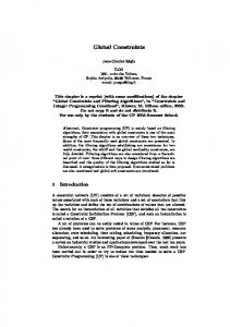
Figure 1: A miter circuit SAT-based bounded sequential equivalence checking is a special case of bounded model checking, where the property is on trying to check if the miter circuit output is a constant 0 from an initial state. The miter circuit is built by connecting a sequential circuit to its optimized version in the following manner. The corresponding primary inputs are tied together, and the corresponding primary outputs are connected by XOR gates. Then all XOR gates are connected to an OR gate. Figure 1 shows the model of our miter circuit. Similar to BMC, the miter is unrolled k time frames, and the equivalence property is checked on the bounded time frames. Our lightweight
G3
G7
G4
G6
Figure 2: Combinational portion of a sequential circuit Vector V1 V2 V3 V4
Table 4: Mining database G1 G2 G3 G4 G5 G6 0 0 X 0 0 X 0 1 X 0 0 X 1 0 X 0 0 X 1 1 X 1 1 1
G7 0 0 0 1
By setting a threshold, we can use the mining algorithm to compute the global constraints from the table. However, the mining constraints obtained will be probabilistic, and we need to verify if they are true global constraints in the sequential circuit via an additional verification check, which is described in Section 3.2.
3.1
Global constraint mining framework
Our framework of mining multi-node relationships is shown in Figure 3. First, a miter circuit is constructed from the sequential circuit and its optimized version. Then the circuit is unrolled to k time frames. M random input vectors are generated and applied to the circuit, and the logic value of each gate is recorded in the mining database. When performing logic simulation, the initial state of PPIs is always set to don’t cares. This is because we are interested in finding potential 3-node relationships that do not depend on any state. Thus, the signal relationships we obtain will be more likely to be globally true. The mining database is thus obtained, where one dimension lists the circuit nodes, and the other dimension lists the vectors. What we perform next is to mining the 3-node constraints from the database. Unlike general data mining where an item is either in or out of a transaction, in our work, we need to learn relations among signals with both logic 0 or logic 1 values. Furthermore, as each item (gate) is 3-valued, the don’t-care value indicates that the node is absent from that entry in the database. To capture the effect of both logic 0 and 1 values, we need to find association rules for both logic 0 and 1. We first compute the
745
Start
Note that the cones may cross several time-frame boundaries. After computing the implication gates for each pair of gates, we check the consistency of implication gates. That is, we check the implication gates’ value in the database to see if it is consistent with every vector that was simulated. In Algorithm 1 below, we describe the procedure of consistency checking.
Creat miter circuit, unroll it to k time frames
Perform logic simulations, generate mining database Mine 3−node constraints Pick one constraint Perform induction based verification
Real
Discard
Record it to constraint table
All constraints verified ?
End
Figure 3: Mining framework signal probability of 0 and 1 for each gate with respect to the random test set. For each gate gi , the probability of gi having logic 0, (Pi0 ), and the probability of gi having logic 1, (Pi1 ), are computed as follows: Pi0 =
(gi = 0)/M
Pi1 =
(gi = 1)/M
where M is total number of vectors simulated. After Pi0 and Pi1 have been computed, we check if the probability is within the following range: Piv ≤ threshold. If so, we mark it as a candidate gate. In our experiments, we set the threshold to be 0.1. The reason for choosing this threshold is that the corresponding controllability values of these nodes are very low. Therefore, assigning a value to the gate might be regarded as difficult, and the constraints we learned are more likely to be hard-to-learn relationships. As we will see from the experiments, such constraints are very useful for the SAT solver. After obtaining the initial candidate gate list, we will mine the potential candidate pairs from the database. Only those pairs whose combinations appear in the database within the same probability ranges are selected, as explained earlier on mining association rules. In addition, when we choose the candidate pairs, we check the two gates’ fanin gate lists. We favor constraints that involve nodes that are not locally close; thus, we want to avoid choosing nodes that have common fanin nodes or if one node is a successor of the other because those are considered local relationships. We are interested in global relationships. For each selected candidate pair (a, b), we will find potential implied gates by the pair. We build fanout cones of a and b, then we calculate the overlapping area; only those gates in the overlapping area are considered for the potential implication.
Algorithm 1 Check consistency // Given a selected pair of gates (g1=val1, g2=val2), // mining database is db, implication gate value is impVal, // M is total number of simulation vectors. for (int i = 1; i ≤ total number of gates; ++i) do if (i in implication gate checklist) then impV al = X; for (int j = 0; j < M ; ++j) do if ((db[j][g1]==val1) && (db[j][g2]==val2)) then if (db[j][i] �= X && impV al = X) then impV al = db[j][i]; else if ((impV al = 0) && (db[j][i] = 1)) then impV al = Invalid; break; else if ((impV al = 1) && (db[j][i] = 0)) then impV al = Invalid; break; end if end if end for end if //save consistent implication gate to implication gate list if (impV al == 0 || impV al == 1) then implication gate list.push back(i); end if end for For example, if the pair of gates is (a = 1 and b = 1), and gate c is a candidate implication gate, we check gate c’s logic value for all a = 1 and b = 1 conditions in the database. If in all cases where a = 1 and b = 1, c appears in only one polarity, then we consider c as a consistent gate. If c = 0, then the potential relationship is a · b → c; if c = 1, then the relationship is a · b → c. We skip the c = X instances. We record all these potential consistent 3-node constraints. The detail of this 3-node constraint mining algorithm is show in Figure 4.
3.2
Validity check of the mined constraints
We need to verify each mined constraint to determine if the constraint is indeed globally correct. We do so by leaving all initial PPIs’ states unconstrained. For example, if the potential constraint a · b → c, we add 3 clauses (a) (b) (¬c) to the original CNF formula of the unrolled miter circuit. If the SAT solver returns UNSAT for the augmented CNF formula, then a · b → c is indeed a globally true constraint, since the validity check puts no constraints on the initial state value. On the other hand, if the SAT solver returns a satisfiable assignment, no conclusion can be made for this 3-node relationship. And those relationships are discarded. We use zChaff [21] as the underlying SAT solver because it supports incremental SAT solving, where portions of clauses can be added or deleted from the database after each run based on their group ID. So we can easily add and delete the augment clauses from the original CNF formula. This could greatly reduce the overhead in checking the validity of the mined global constraints.
746
Database
4.
Perform 1st mining iteration Construct pair of nodes
Have same fanin gate
Y
Skip this pair
N Perform 2nd mining iteration Build fanout cone of gate pair, find all gates in overlapping area
Put the gates in implication list check consistency Save all potential 3−nodes constraints
Figure 4: 3-node mining flow
3.3 Application to bounded sequential equivalence checking The global constraints learned can be applied to various verification problems. In our work, these constraints are applied to bounded sequential equivalence checking between an original sequential circuit with its optimized version. Note that these constraints are global invariants, so the replicated constraints are also added to successive time frames. For example, consider that the mining is applied to a 4-time-frame unrolled miter. If a learned constraint involves node a in time frame #1 and node b in time frame #3 imply node c in time frame #4: a1 · b3 → c4 . Then, this constraint can be replicated to more deeply unrolled miters as well. For instance, the replicated constraint a3 · b5 → c6 is also valid and can be added to the formula. Zchaff is again used as underlying SAT solver. The sequential equivalence checking model is shown in Figure 5, where each time frame consists of both the original and optimized circuits. All initial states are set to 0, and the verification is on checking if the miter output can be satisfied to 1.
Figure 5: Bounded equivalence checking model
EXPERIMENTAL RESULTS
The proposed technique was implemented in C++. All tests were performed on a Pentium IV, 2.8 GHz, with 1GB of RAM, running the Linux Redhat v9. The ISCAS’89 and ISCAS’93 addendum benchmarks, along with their Synopsys-optimized circuits are used in our bounded sequential equivalence checking. Equivalence checking on some ISCAS benchmarks was very easy for the SAT solver; For such easy benchmarks, adding constraints using our approach will not improve the results. Thus, we exclude those easy benchmarks in our experimental results and only report the hard miters. We compare the SAT solving time with and without adding the learned 3-node constraints. First, Table 5 shows the mining results. The first column shows the miter circuits used. The second column reports how many time-frames the miter circuit was unrolled. While stronger constraints could be discovered in more deeply unrolled circuits, the mining time must also be considered to keep the learning cost low. We chose the number of time frames to keep the total number of nodes in the unrolled circuit between 10,000 to 500,000. Experimental results show that within this range the mining time is kept low, yet the global constraints learned is powerful enough. The third column reports the number of true constraints identified for each benchmark. The fourth column reports the percentage of real constraints of all potential constraints. The last column reports the total mining time in seconds. For instance, in miter-circuit s4863 with its optimized circuit, the learning is performed on a 7-time-frame unrolled miter, 4831 3-node true global constraints were learned. This is 79% of all mined relationships. Note that this percentage depends on the threshold values used in the mining algorithm. Finally, the total learning time was 147.84 seconds. Miter s298 s832 s1196 s1488 s3330 s4863 s5378 s15850 s35932 s38584
Table 5: Mining Results # time frames True clauses % 40 56 86 20 40 95 20 1020 71 20 229 33 7 225 75 7 4831 79 7 3443 40 7 5087 81 5 6245 76 5 8050 82
Time (s) 15.4 31.47 85.21 122.04 103.6 147.84 247.53 562.17 1094.34 2566.95
Before we apply these constraints to bounded sequential equivalence checking, we will first discuss the efficiency of our learning method. Table 6 compares the computation complexity of our method with a naive method. The naive method explores all possible 3-node combinations, whose complexity is n(n−1)(n−2) , where n is the number of nodes in the un6 rolled miter circuit. The column “3-node mining” shows total number of 3-node relationships selected by our mining algorithm. The last column reports the number of relationships using the naive 3-node combinations. From this table we can see that even for a very small circuit s298, the total number of 3-node combinations is already very large. It will easily cause both memory and temporal explosion, and completing such searches for global constraints will be infeasible. On the other hand, our mining algorithm is shown to be very efficient, with the computation complexity growing linearly with the circuit size.
747
6.
Table 6: Comparison of computation complexity # time Total # Our 3-node All 3-node Miter frames nodes mining combinations s298 40 9948 65 1.64 × 10¹¹ s832 20 11670 42 2.64 × 10¹¹ s1196 20 20716 1437 5.06 × 10¹¹ s1488 20 24052 694 2.32 × 10¹² s3330 7 27963 300 3.64 × 10¹² s4863 7 27004 6115 3.28 × 10¹² s5378 7 42372 8607 1.27 × 10¹³ s15850 7 147081 6280 5.30 × 10¹⁴ s35932 5 183171 8217 1.02 × 10¹⁵ s38584 5 211414 9817 1.57 × 10¹⁵ Finally, Table 7 shows the result of applying the learned constraints to bounded sequential equivalence checking. Because we are checking the equivalence of a sequential circuit with its optimized version, all results are UNSAT.1 For each miter circuit, the number of time frames is first reported. Note that the number of time-frames unrolled here can be different from the number of time-frames used to learn the constraints as reported in Table 5. The third column reports the original execution time of the SAT solver without adding any constraints. Next, the SAT solving time after adding global constraints is reported, followed by the total time (mining + equivalence checking). Finally, speedup is reported. Note that all times are reported in seconds. From the results we can see that in most cases the constraints could speed up the SAT solving time significantly. Noteworthy improvements were achieved for all miter circuits: in 6 of the 10 cases, more than one order of magnitude speedup was obtained; in the s3330 miter, more than 2 orders of magnitude speed was achieved. Table 7: Bounded sequential equivalence Checking Miter s298 s832 s1196 s1488 s3330 s4863 s5378 s15850 s35932 s38584
5.
# time frames 40 30 30 30 15 15 15 15 10 10
original (s) 48.24 1594.55 221.31 4187.11 >86400 6594.76 8248.53 23057.20 4984.37 8832.45
new (s) 0.1 0.23 0.32 1.35 28.62 289.68 129.9 10.28 3.28 4.63
mining + new (s) 15.5 31.7 85.53 123.39 132.22 437.52 377.43 572.45 1097.62 2571.58
Speedup 3.11 50.30 2.59 33.93 >653.46 15.07 21.85 40.28 4.54 3.43
CONCLUSIONS
We presented a novel mining technique to quickly identify global constraints in sequential circuits. The proposed mining method allows us to efficiently identify the useful global constraints in the huge number of possible relationships in the circuit. Experiments show that the proposed mining strategy is very efficient in identifying important multi-nodes relationships that can significantly enhance the SAT solver in a bounded sequential equivalence checking framework. One to two orders of magnitude speedup was achieved for many cases. Future work includes exploring mining for relationships that involve more than 3 nodes as well as application to general model checking instances. 1 Equivalence check of buggy optimized designs was very easy for the SAT solver, thus they are not included.
REFERENCES
[1] M. H. Schulz, E. Trischler and T. M. Sarfert. SOCRATES: A highly efficient automatic test pattern generation system. IEEE Trans. CAD, vol. 7, no. 1, Jan. 1988, pp. 126-137. [2] W. Kunz and D. K. Pradhan. Accelerated dynamic learning for test pattern generation in combinational circuits. IEEE Trans. CAD, vol. 12, no. 5, May 1993, pp. 684-694. [3] H. Ichihara and K. Kinoshita. On acceleration of logic circuits optimization using implication relations. In Proc. Asian Test Symp., 1997, pp. 222-227. [4] W. Kunz, D. Stoffel and P. R. Menon. Logic optimization and equivalence checking by implication analysis. IEEE Trans. CAD, Vol. 16 , no. 3, Mar. 1997, pp.266-281. [5] S. Kajihara, K. K. Saluja and S. M. Reddy. Enhanced 3-valued logic/fault simulation for full scan circuits using implicit logic values. Proc. European Test Symp., 2004, pp. 108-113. [6] M. E. Amyeen, W. K. Fuch, I. Pomeranz and V. Boppana. Implication and evaluation techniques for proving fault equivalence. Proc. VLSI Test Symp., 1999, pp. 201-207. [7] W. Kunz, D. Pradhan and S. Reddy. A Novel Framework for Logic Verification in a Synthesis Environment. IEEE Trans. CAD, vol. 15, no. 1, Jan. 1996, pp. 20-32. [8] M. lyer and M. Abramovici. FIRE: A Fault-independent Combinational Redundancy Identification Algorithm. IEEE Trans. VLSI Systems., vol. 4, no. 2, Jun. 1996, pp. 295-301. [9] J. K. Zhao, M. Rudnick and J. Patel. Static Logic Implication with Application to Fast Redundancy Identification. Proc. VLSI Test Symp., 1997, pp. 288-293. [10] M. H. Schulz and E. Auth. Improved deterministic test pattern generation with applications to redundancy identification. IEEE Trans. CAD, vol. 8, no. 7, Jul. 1989, pp. 811-816. [11] Y. Novikov. Local search for Boolean relations on the basis of unit propagation, Proc. Design, Automation and Test in Europe Conf., 2003, pp. 810-815. [12] J. Rajski and H. Kox. A Method to Calculate Necessary Assignments in ATPG. Proc. Int’l. Test Conf., 1990, pp. 25-34. [13] S.T. Chakradhar and V. D. Agrawal. A transitive closure algorithm for test generation. IEEE Trans. CAD., 1993, pp. 1015 - 1028. [14] W. Kunz and D. K. Pradhan. Recursive Learning: A new Implication Technique for Efficient Solutions to CAD problems test, verification, and optimization. IEEE Trans. CAD., 1993, pp.1149-1158. [15] J. Zhao, J. A. Newquist and J. Patel. A graph traversal based framework for sequential logic implication with an application to c-cycle redundancy identification. Proc. VLSI Design Conf., 2001, pp. 163-169. [16] K. Gulrajani and M. S. Hsiao. Multi-node static logic implications for redundancy identification. Proc. Design, Automation, and Test in Europe Conf., 2000, pp. 729-733. [17] M. Syal, R. Arora and M. S. Hsiao. Extended forward implications and dual recurrence relations to identify sequentially untestable faults. Proc. Int’l Conf. Computer Design, 2005, pp. 453-460. [18] D. J. Hand, H. Mannila and P. Smyth. Principles of Data Mining. MIT Press, Aug. 2001. [19] A. Biere, A. Cimatti, E. M. Clarke, M. Fujita and Y. Zhu Symbolic model checking using SAT procedures instead of BDDs. Proc. Design Automation Conf., 1999, pp. 317-320. [20] A. Kuehlmann. Dynamic Transition Relation Simplification for Bounded Property Checking. Proc. Int. Conf. Computer-Aided Design., 2004, pp. 50-57. [21] M. Moskewicz, C. Madigan, Y. Zhao, L. Zhang and S. Malik. Chaff: Engineering an efficient SAT solver. Proc. Design Automation Conf., 2001, pp. 530-535. [22] E. Goldberg and Y. Novikov. BerkMin: A fast and robust Sat Solver. Proc. European Design and Test Conf., 2002, pp. 142-149. [23] F. Lu, L. C. Wang and K. T. Cheng. A circuit SAT solver with signal correlation guided learning. Proc. European Design and Test Conf., 2003, pp. 892-897. [24] R. Agrawal, T. Imielinski and A. Swami. Mining association rules between sets of items in large databases. Proc. Conf. Management of Data, 1993, pp. 207-216. [25] R. Agrawal, T. Imielinski and A. Swami. Database mining: A performance perspective. IEEE Trans. Knowledge and Data Engineering, vol. 5, No. 6, 1993, pp. 914-925.
748