represents a potential interaction), while the state of each interaction ...... [12] H. Kwak, C. Lee, H. Park, and S. Moon, âWhat is twitter, a social network or a news ... [14] J. Diesner, T. L. Frantz, and K. M. Carley, âCommunication. Networks from ...
Mining Heavy Subgraphs in Time-Evolving Networks Petko Bogdanov† , Misael Mongiov`ı† , Ambuj K. Singh Department of Computer Science, University of California Santa Barbara, CA 93106-5110 Email: {petko,misael,ambuj}@cs.ucsb.edu
Abstract—Networks from different genres are not static entities, but exhibit dynamic behavior. The congestion level of links in transportation networks varies in time depending on the traffic. Similarly, social and communication links are employed at varying rates as information cascades unfold. In recent years there has been an increase of interest in modeling and mining dynamic networks. However, limited attention has been placed in high-scoring subgraph discovery in timeevolving networks. We define the problem of finding the highest-scoring temporal subgraph in a dynamic network, termed Heaviest Dynamic Subgraph (HDS). We show that HDS is NP-hard even with edge weights in {−1, 1}, and devise an efficient approach for large graph instances that evolve over long time periods. While a na¨ıve approach would enumerate all O(t2 ) sub-intervals, our solution performs an effective pruning of the sub-interval space by considering O(t · log(t)) groups of sub-intervals and computing an aggregate of each group in logarithmic time. We also define a fast heuristic and a tight upper bound for approximating the static version of HDS, and use them for further pruning the sub-interval space and quickly verifying candidate sub-intervals. We perform an extensive experimental evaluation of our algorithm on transportation, communication and social media networks for discovering subgraphs that correspond to traffic congestions, communication overflow and localized social discussions. Our method is two orders of magnitude faster than a na¨ıve approach and scales well with network size and time length.
fields. Extending the notion of high-scoring subgraphs to time-evolving networks can enable several interesting applications. For example, the road network is characterized by a fixed network topology whose edge utilization varies with time according to traffic [7]. High scoring sub-networks correspond to congested locations over an extent in time. Similarly, in the biological domain, the activity within a cell can be represented as a network of interactions between cell components (DNA, proteins, RNA, small molecules). The network structure is fixed (an edge between two components represents a potential interaction), while the state of each interaction (active/inactive) changes during the execution of biological processes [8]. Finding a connected set of active interactions that persist in time is useful to identify functional modules and analyze their evolution in time [9]. In this paper we introduce the Heaviest Dynamic Subgraph (HDS) problem, i.e. the problem of finding the highest-scoring connected temporal subgraph in an edgeweighted network whose weights evolve in time (edgeevolving network for short). A temporal subgraph is characterized by its participating edges and a time sub-interval. The score of a temporal subgraph is defined as the sum of the edge weights. Our problem can be naturally extended to finding the top-k high-scoring non-overlapping subgraphs.
I. I NTRODUCTION Time-evolving networks arise in multiple application domains. They can characterize traffic variation in transportation networks, information flow in communication networks, variation of trade rates in a network of trading agents or phases of pathway switching in gene interaction networks. Despite their rich representative power, time-evolving networks have received limited attention from the data mining and database communities. Most existing dynamic network research focuses on link formation [1] and community discovery [2], [3]. Limited attention has been placed to the problem of finding high scoring subgraphs in time-evolving networks. Approaches for finding high-scoring subgraphs have been widely studied for static networks [4], [5]. They have many applications in Biology [4], network design [6] and other † These
authors contributed equally to this work
Figure 1. An example of time-evolving network (a). Edges in each time step are scored either 1 or −1 (solid or dashed, respectively). The heaviest subgraph is defined over the sub-interval [1, 3] and consists of edges AC, AB, BE (b). (c) shows the scoring of the same subgraph in the interval [1, 4]
An example for HDS is depicted in Fig. 1(a). Solid lines
represent edges with score 1, while dashed lines represent edges of score −1. A possible social network interpretation is the unfolding of a discussion among friends over time. At the beginning the pairs {(C, D)(A, C), (A, B), (E, B)} initiate a discussion. Although B “knows” C, they do not interact directly in this discussion. The discussion then persists for pairs (A, C) and (E, B) (steps 2 and 3) and terminates at step 4. The heaviest dynamic subgraph in this example is the set of edges AB, AC, BE over the sub-interval [1, 3]. HDS captures the backbone of communication channels employed in the discussion process, while excluding the edges that are not used (such as BC). Similar interpretations can be derived for transportation and biological networks. HDS balances the cost of considering negative edges with the benefit of connecting high-scoring components. For example in Fig. 1, the edges AC and BE are connected through the edge AB even though its weight is prevalently negative. Joining the two edges is advantageous since it produces a larger temporal subgraph whose overall score (value 5) is higher than the score of the single temporal subgraphs (value 3 each). Admitting solutions that contain negative edges has several advantages. First, since weights change over time, not admitting negative edges would tend to discard longer sub-intervals. Second, in many applications, it may be worthwhile to pay a small cost for producing a larger component. Finally, it makes the method robust to noise, since sporadic negative values resulting from noise do not significantly affect the result. A na¨ıve method for solving HDS would reduce the problem to the static case by enumerating all the possible t·(t+1) 2 time sub-intervals and finding the highest-scoring subgraph in each one of them. However, this approach would not scale for two main reasons. First, the number of sub-intervals is quadratic in the length of the time interval. Second, finding the highest-scoring subgraph in a static network is NPhard, thus solving it optimally is infeasible on large graphs. Although efficient heuristics exist [10], executing them on each sub-interval would be infeasible for large HDS problem instances. Reducing the quadratic dependence on the time length is a challenge, since neither the optimal score is convex in the sub-interval space nor the score of an interval can be related to the score of sub-intervals. We propose a novel filter-and-verify approach for pruning sub-intervals named MEDEN (Mining EDge-Evolving Networks). Besides defining tight bounds of the optimal solution for pruning sub-intervals that are not promising, we introduce a novel sub-interval aggregation scheme that allows us to prune groups of sub-intervals without inspecting their members. Our filtering method has complexity O(t · log 2 (t) · |E|), where t is the total time length of the graph evolution. Our method achieves high pruning power by guaranteeing that only highly overlapping subintervals are grouped together. We propose a fast heuristic for the verification phase. We experiment extensively with
our method on several real and synthetic datasets and show that it scales well with time length and network size. Our contributions include: 1) we formulate the HDS problem and prove that it is NP-hard even with edge weights in {−1, 1}; 2) we design a filter-and-verify approach for HDS based on a tight upper bound for the optimal solution in a specific sub-interval; 3) we propose a novel sub-interval aggregation scheme and give an effective method for pruning the quadratic sub-interval space in time O(t · log 2 (t) · |E|); 4) we introduce an efficient heuristic for verifying promising sub-intervals that scales with the graph size; 5) we experiment with our method on dynamic networks of different genres and sizes and demonstrate its scalability. The rest of this paper is structured as follows: We formally define the HDS problem in section II. We develop a filterand-verify solution for HDS that relies on a scalable heuristic and a tight upper bound in Section III. Our space partitioning scheme and scalable mining algorithm MEDEN are developed in Section IV. Section V presents experimental results and section VI discusses related work. We conclude in Section VII. II. P RELIMINARIES AND P ROBLEM F ORMULATION In this section we first define the problem Heaviest Subgraph (HS) for static graphs and discuss its relation to the known Prize-Collecting Steiner Tree (PCST) problem [4]. We then define HDS for time-evolving networks and show that it is NP-hard. ¯ = Definition 2.1: Given an edge-weighted graph G (V, E, w), the Heaviest Subgraph (HS) problem calls for ¯ 0 = (V 0 , E 0 ) of G ¯ such as its score, finding a subgraph G P defined as e∈E 0 w(e) is maximal. ¯ = The PCST problem [10] takes as input a network G (V, E, w), with positive vertex weights and negative edge weights1 . There are two different formulations of this problem. The Goemans-Williamson Minimization (GW-PCST) finds the connected subgraph that minimizes the sum of the node weights that are not included in the solution minus the sum of the edge weights within the solution. More 0 0 ¯0 precisely, the score of aPconnected subgraph P G = (V , E ) ¯ of G = (V, E, w) is v∈V \V 0 w(v) − e∈E 0 w(e). The Net Worth Maximization (NW-PCST) maximizes the score P P w(v) + w(e). Although the optimal solutions 0 0 v∈V e∈E of the two formulations are equivalent, GW-PCST can be 1 using GW-algorithm [10], approximated to a factor 2 − n−1 while NW-PCST cannot be approximated polynomially within any constant factor [11]. 1 In [10] edge weights are defined to be positive and their score is inverted in the scoring function.
HS and PCST can be reduced to each other in linear time. HS can be reduced to PCST by collapsing all the connected components with positive edges in one node with weight equal to the sum of the weights of the collapsed edges. Similarly, PCST can be reduced to HS by adding a new edge per node and assigning the node weight to it. Formal proofs of these reductions are omitted for space reasons. For convenience, we define a summation (+) and max operators for edge-weighted graphs as follows. ¯ 1 = (V, E, w1 ) and G ¯2 = Definition 2.2: Let G (V, E, w2 ) be two edge-weighted isomorphic graphs that may have different edge weights. We define (i) the aggre¯ = G ¯1 + G ¯ 2 as G ¯ = (V, E, w) such that gate graph G w(e) = w1 (e) + w2 (e), ∀e ∈ E and (ii) the domination ¯ M = max(G ¯1, G ¯ 2 ) as G ¯ M = (V, E, wM ) such that graph G wM (e) = max(w1 (e), w2 (e)), ∀e ∈ E. Both operators can also be applied to sets of graphs. Next, we introduce the Heaviest Dynamic Subgraph (HDS) problem and state that it is NP-hard. Definition 2.3: An edge-evolving network G = (V, E, F ) is an undirected connected graph where V is the set of vertices, E is the set of edges, and F = {f 1 , f 2 , . . . , f |F | } is a family of functions of the kind f i : E → {−1, 1} that associate each edge e ∈ E with a weight. Each function f i is associated with a discrete timestamp i. Note that we restrict the edge weights to assume values in {+1, −1}. Below we prove that, even in this case, the problem is NP-hard. Due to its simplicity, combined with expressiveness, we adopt this scheme in the rest of the paper. Our method and results are naturally applicable to timevarying networks with arbitrary edge weights. Definition 2.4: A temporal subgraph of an edge-evolving network G = (V, E, F ) is a pair (G0 = (V 0 , E 0 ), [i, j]), where G0 is a connected subgraph of G and [i, j] is a subinterval of [1, |F |], i.e. 1 ≤ i ≤ j ≤ |F |. The score of G0 is defined as: score(G0 , i, j) =
X
j X
f k (e)
e∈E 0 k=i
Definition 2.5: The HDS problem is defined as finding the temporal subgraph (G0 , [i, j]) of an edge-evolving network G such that score(G0 , i, j) is maximal. HDS is an optimization problem in which the scoring function has to be maximized over all possible subgraphs G0 ∈ G and all possible sub-intervals of the whole interval. Note, that the HDS formulation allows for parameter-free discovery of high-scoring solutions that are either small subgraphs with a large time extent or large subgraphs with a smaller time extent. The score of a temporal subgraph can be informally considered as the importance of the process that it represents. For example, the importance of a congestion may be considered high due to either its long time duration or the size of the road network that it affects.
Theorem 2.1: HDS is NP-hard. The proof of NP-hardness is based on a reduction from the Minimum Thumbnail Rectilinear Steiner Tree (TRST) problem, a variant of Minimum Steiner Tree in which nodes are embedded in a 2D grid and segments are restricted to be horizontal or vertical. The reduction considers a grid graph that represents the TRST grid and a high-scoring path for each terminal point of the TRST. The formal proof is omitted due to space limitation. Definition 2.6: Given an edge-evolving network G = (V, E, F ) and a sub-interval [i, j] with i, j ∈ {1, 2, . . . |F |}, we define the aggregated graph induced by P [i, j] as the j k ¯ j) = (V, E, w), where w(e) = graph G(i, k=i f (e) is a function that associates edges with the sum of their respective weights in [i, j]. HDS can be solved by enumerating all the possible subintervals [i, j] of [1, |F |] and solving HS on the aggregated graph induced by each sub-interval. This solution, however, = would require solving the NP-hard HS problem t·(t+1) 2 O(t2 ) times, and hence would not scale with time length. Although HS is equivalent to PCST (in static networks), this result is not generalizable to HDS with arbitrary edge weights. Consider the natural extension of PCST to dynamic networks (let’s call it dynamic PCST), i.e. the problem of finding the highest-scoring temporal subgraph in a timeevolving network with positive node weights and negative edge weights. An instance of dynamic PCST can be reduced to HDS with arbitrary edge weights by repeating the process slice by slice. A similar reduction from an instance of HDS to an instance of dynamic PCST is not possible since it would require considering a different network structure for each slice. For this reason, we focus on HDS as a more general problem than dynamic PCST. Clearly all the results in this paper extend to dynamic PCST. III. A FILTER - AND - VERIFY FRAMEWORK FOR HDS An HDS solution is characterized by two main dimensions (i) subgraph: the set of edges forming a connected subgraph and (ii) time extent: a sub-interval. Since the problem in the time dimension can be solved by multiple applications of the Heaviest Subgraph (HS) problem for static graphs and this last problem is NP-hard (Theorem 2.1), we first present our heuristic for HS. We then develop an efficient filtering solution to prune the quadratic sub-interval space. The combination of the two components gives a Basic filterand-verify procedure for HDS. A. A heuristic for Heaviest Subgraph (HS) In this section we propose TopDown, a scalable heuristic for solving HS. TopDown’s performance is comparable to GW-algorithm (applied after reducing HS to PCST, Section II). While neither TopDown nor GW-algorithm can guarantee a constant factor approximation for our scoring
Algorithm 1 TopDown ¯ = (V, E, w) Input: An edge-weighted graph G 0 ¯ ¯ Output: an HS solution G ⊆ G ¯ 1: T ← Max. Spanning Tree of G 2: Move positive weights to adjacent nodes in T 3: T 0 ← NW-PCST-Tree(T ) 4: G0 ← T 0 ∪{Positive edges, adjacent to T 0 } 5: return G0
function, TopDown has the advantage of lower time complexity. Our approach is flexible, allowing to use either heuristic, according to the desired trade-off between quality and efficiency. TopDown obtains a global solution by initially including ¯ and refining it by excluding non-optimal all nodes in G subgraphs (Algorithm 1). In Step 1 we compute a Maximum ¯ Next, we Spanning Tree T of the edge-weighted graph G. construct a tree instance of NW-PCST by moving the weight of each positive edge to one of its adjacent nodes in T (Step 2). Although NW-PCST is hard to approximate for general graphs, it can be computed exactly on trees in time linear in the number of nodes. NW-PCST-Tree (Step 3) is equivalent to the strong pruning phase of the PCST approximation by Johnson et al. [10]. It computes the spanning tree PCST solution T 0 which is then expanded to G0 by restoring the original edge weights and adding all positive edges adjacent to T 0 (Step 4). The complexity of TopDown is dominated by the Maximum Spanning Tree construction (Step 1), which can be performed by Prim’s algorithm in time O(|E| · log(|V |)) using a binary heap, or in time close to linear in the number of edges due to later improvements. In contrast to TopDown, GW-algorithm [10] has a super quadratic running time O(|V |2 · log |V |). In our experimental analysis, TopDown achieves on average more than 90% of the best score computed by GW-algorithm. Any of the two algorithms can be used in our overall solution for HDS. B. Upper bounds for HS A na¨ıve approach for HDS would solve HS in all t(t−1) 2 sub-intervals. The complexity can be reduced by quickly pruning non-promising sub-intervals. The pruning procedure bounds the solution in each sub-interval and discards the sub-intervals whose upper bound is smaller than a previously found solution. A simple upper bound, named U Bsop (sumof-positive), can be obtained by summing all the positive edges. Although U Bsop is very fast and can be used for a first screening, it is not tight due to many positive edges distributed on a graph. We define a tighter upper bound, U Bstr (structural), by relaxing the graph structure and connecting the positive components “optimistically”. ¯ = (V, E, w) be an edge-weighed Lemma 3.1: Let G 0 ¯ graph and G be an optimal solution for HS with score s.
Algorithm 2 Basic Input: An edge-evolving graph G(V, E, F ) Output: (G0 , [i, j]), a solution for HDS 1: Compute U BSOP , ∀[l, r] ∈ [1, |F |] 2: Estimate a Lower Bound LB for HDS 3: for all [l, r] ∈ [1, |F |] do 4: Prune [l, r] if U BSOP ≤ LB or U BST R ≤ LB 5: end for 6: for all Not pruned sub-intervals [l, r] do ¯ r)) 7: T opDown(G(l, 8: end for 9: return The highest-score temporal subgraph (G0 , [i, j])
Let also C = {(P, N )} be a set of pairs where P represents ¯ the score of a connected component of positive edges in G and N represents the lowest score among negative edges with one endpoint in the corresponding positive component. We have: X U BST R = max(0, P + N ) − min (N ) ≥ s (P,N )∈C
(P,N )∈C
We do not report the proof due to space limitations. Since U BST R preserves more structural information, it is significantly tighter than U BSOP . When the positive components in G are “close” to each other, U BST R is close to the score of the optimal solution. The time necessary to compute both U BSOP and U BST R , is linear in the number of graph edges. In practice U BSOP takes much less time and both bounds are significantly faster than TopDown. As we show in the experimental evaluation, both upper bounds have good pruning power in real and synthetic problem instances. C. A filter-and-verify algorithm for HDS A filter-and-verify approach for HDS, called Basic, which uses the developed bounds is presented in Alg. 2. Basic takes as input an edge-evolving network. In Step 1 we compute U BSOP for all O(t2 ) sub-intervals. Next, we estimate a lower bound LB for HDS by applying TopDown on the k sub-intervals that have the highest U BSOP (Step 2 ). The intuition is that if a sub-interval induces many positive edges it is likely to contain a good solution. sub-intervals proIn Steps 3-5 we check each of the t(t−1) 2 gressively and prune irrelevant sub-intervals by first applying U BSOP and then U BST R . All intervals that are not pruned are next verified by using TopDown (Steps 6-8). We maintain the best temporal subgraph (G0 , [i, j]) from all applications of TopDown and return it as the solution (Step 7). Since U BSOP and U BST R are upper bounds for HS, the filtering procedure does not have any loss in quality. Basic reduces the running time by orders of magnitude with respect to a na¨ıve solution by discarding most of the search space. However, Basic does not scale well with the time length
t, as it requires the computation of U BSOP for all O(t2 ) intervals. We reduce the complexity of the initial filtering phase to O(t·log2 (t)·|E|) by grouping intervals, as described in the next section. IV. S CALABLE FILTERING BY SUB - INTERVAL GROUPING In this section we define a sub-interval aggregation scheme that partitions the quadratic space of candidate subintervals into O(t · log(t)) disjoint groups. We introduce a fast filtering phase that prunes groups without considering their individual members and hence has a sub-quadratic complexity of O(t · log 2 (t) · |E|). The grouping of subintervals follows an intuitive principle: sub-intervals with significant overlap produce similar aggregated graphs and hence solutions of similar score. Our final algorithm for HDS, called MEDEN, achieves an order of magnitude improvement over Basic (Alg. 2) in our experiments. A. Aggregation scheme The sub-interval aggregation scheme maintains a constant minimum fraction of overlap for any pair of sub-intervals within the same group. Groups are composed of left-aligned sub-intervals, i.e. sub-intervals that share the same starting point. To ensure a minimum overlap of α (with 0 ≤ α < 1) within groups, we combine short sub-intervals in smaller size groups and larger sub-intervals in larger size groups. The relationship between the number of groups and interval length has an exponential form, ensuring that the total number of disjoint groups is O(t · log(t)). We define the fraction of overlap between two subintervals as the ratio of the lengths of their intersection and union. The overlap varies between 0 (the sub-intervals do not intersect) to 1 (the sub-intervals are exactly the same). A left-aligned group S(i, k1 , k2 ) is a group of subintervals that start from the same position i and end at positions k1 through k2 , k2 ≥ k1 . Formally: S(i, k1 , k2 ) = {[i, j]|k1 ≤ j ≤ k2 }. The minimum overlap in a group of left-aligned subintervals S(i, k1 , k2 ) is the ratio between the minimum and maximum length of intervals within the group, i.e. (k1 − i + 1)/(k2 − i + 1). Let G = (V, E, F ) be an edge-evolving network with total time period t = |F |. Let α be the minimum admitted overlap within a group. For every position i, 1 ≤ i ≤ t, we divide the sub-intervals starting at i in left-aligned groups as follows: j 1 k � n � j 1 k i , i + − 1, t SG,α = S i, i + αj−1 αj j 1 k j 1 k o[ ≤ − 1 1 ≤ j ≤ n − 1 and αj−1 αj
n � �o [ n � j 1 k �o S i, i, i S i, i + ,t , αn−1 j k where n is the smallest integer satisfying i + α1n − 1 ≥ t. The key concept in the above aggregation strategy is that the set of all left-aligned intervals starting at i is divided in a logarithmic number of groups, since the difference between the earliest and latest interval ends within a group grows exponentially with the group index j. We also consider the extreme cases S(i, i, i) and S(i, i+b1/αn−1 c, t) for the sake of completeness. Building on the partitioning for one starting point, we define the complete partition of intervals for G as SG,α = S i 1≤i≤t SG,α . Clearly all sub-intervals of [1, t] are included in at least one set of SG,α and the sets are mutually disjoint. The following lemma states that the aggregation scheme produces a partition of size O(t · log(t)) and the minimum overlap of a pair within each group exceeds α. Lemma 4.1: Let G = (V, E, F ) be a time-varying network (t = |F |), and α be a real value in [0, 1]. Then, the complete partition of intervals SG,α has the following properties: 1) |SG,α | = O(t · log(t)) 2) overlap([i, j], [k, l]) ≥ α, ∀[i, j], [k, l] ∈ S, ∀S ∈ SG,α Proof: 1) Given a starting time i such that 1 ≤ i ≤ i t, by definition |SG,α j| ≤ kn + 1 where n is the minimum
integer satisfying i + α1n − 1 ≥ t. Consequently, we have j k 1 1 i + αn−1 − 1 < t and hence i + αn−1 − 2 < t. We obtain i the following bound for a single starting point: |SG,α | ≤ log(t−i+2) n + 1 < − log(α) + 2. Therefore: |SG,α | =
X
i |SG,α |