Mining Significant Graph Patterns by Leap Search∗ Xifeng Yan]
Hong Cheng†
Jiawei Han†
Philip S. Yu‡
]
†
IBM T. J. Watson Research Center,
[email protected] University of Illinois at Urbana-Champaign, {hcheng3, hanj}@cs.uiuc.edu ‡ University of Illinois at Chicago,
[email protected]
Keywords Graph, Pattern, Optimality, Classification
ABSTRACT
1.
With ever-increasing amounts of graph data from disparate sources, there has been a strong need for exploiting significant graph patterns with user-specified objective functions. Most objective functions are not antimonotonic, which could fail all of frequency-centric graph mining algorithms. In this paper, we give the first comprehensive study on general mining method aiming to find most significant patterns directly. Our new mining framework, called LEAP(Descending Leap Mine), is developed to exploit the correlation between structural similarity and significance similarity in a way that the most significant pattern could be identified quickly by searching dissimilar graph patterns. Two novel concepts, structural leap search and frequency descending mining, are proposed to support leap search in graph pattern space. Our new mining method revealed that the widely adopted branch-and-bound search in data mining literature is indeed not the best, thus sketching a new picture on scalable graph pattern discovery. Empirical results show that LEAP achieves orders of magnitude speedup in comparison with the state-of-the-art method. Furthermore, graph classifiers built on mined patterns outperform the up-to-date graph kernel method in terms of efficiency and accuracy, demonstrating the high promise of such patterns.
INTRODUCTION
Graph data has grown steadily in a wide range of scientific and commercial applications, such as in bioinformatics, security, the web, and social networks. As witnessed in the core tasks of these applications, including graph search and classification, graph patterns could help build powerful, yet intuitive models for better managing and understanding complex structures. Their usage, therefore, is far beyond traditional exercises, such as, association rules. Many powerful data management and analytical tools like R-tree and support vector machine, cannot adapt to the graph domain easily due to the lack of vector representation of graphs. Recent advances in graph mining illustrated that it is not only possible but also effective to vectorize graphs based on frequent subgraphs discovered in a mining process. Given a set of frequent subgraphs1 g1 , g2 , . . ., gd , a graph G can be represented as a vector x = [x1 , x2 , . . . , xd ], where xi = 1 if gi ⊆ G; otherwise, xi = 0. Yan et al. [28] (and Cheng et al. [6]) demonstrated that through such vectorization, efficient indices could be built to support fast search in graphs. In addition to graph search, graph data analysis could benefit from pattern-based vectorization as well. For example, pattern-based support vector machine [7] has been shown achieving promising classification accuracy. Meanwhile, by explicitly presenting significant substructures, these methods provide with users a direct way to understand complex graph datasets intuitively.
Categories and Subject Descriptors H.2.8 [Database Applications]: data mining; I.5.1 [Pattern Recognition]: Models—statistical
bottleneck
General Terms
mine
Algorithms, Performance
exploratory task graph index
select
graph classification
∗The work of H. Cheng and J. Han has been supported in part by the U.S. National Science Foundation NSF IIS-0513678, BDI-05-15813, and an IBM Scholarship.
graph dataset
exponential pattern space
significant patterns
graph clustering
Figure 1: Graph Pattern Application Pipeline Scalability Bottleneck. Figure 1 depicts the pipeline of graph applications built on frequent subgraphs. In this pipeline, frequent subgraphs are mined first and from which, significant patterns are selected based on user-defined ob-
Permission to make digital or hard copies of all or part of this work for personal or classroom use is granted without fee provided that copies are not made or distributed for profit or commercial advantage and that copies bear this notice and the full citation on the first page. To copy otherwise, to republish, to post on servers or to redistribute to lists, requires prior specific permission and/or a fee. SIGMOD’08, June 9–12, 2008, Vancouver, BC, Canada. Copyright 2008 ACM 978-1-60558-102-6/08/06 ...$5.00.
1
Given a graph dataset D = {G1 , G2 , . . . , Gn } and a minimum frequency threshold θ, frequent subgraphs are subgraphs that are contained by at least θ|D| graphs in D. 1
and-bound search in the above search tree and estimate the upper bound of F (g) for all of descendants below each node. If it is smaller than the value of the best pattern seen so far, it cuts the search branch of that node. Under branchand-bound search, a tighter upper bound of F (g) is always welcome since it means faster pruning. Existing optimal pattern mining algorithms followed this strategy. However, we recognized that due to the exponential graph pattern space, the branch-and-bound method could be easily trapped at local maxima. Therefore, instead of developing yet another bounding technique, we are going to explore a general mining strategy beyond branch-and-bound.
jective functions. Unfortunately, the potential of graph patterns is hindered by the limitation of this pipeline, due to a scalability issue. For instance, in order to find subgraphs with the highest statistical significance, one has to enumerate all of frequent subgraphs first, and then calculate their p-value one by one. Obviously, this two-step process is not scalable due to the following two reasons: (1) for many objective functions, the minimum frequency threshold has to be set very low so that none of significant patterns will be missed—a low-frequency threshold often means an exponential pattern set and an extremely slow mining process; and (2) there is a lot of redundancy in frequent subgraphs; most of them are not worth computing at all. Thus, the frequent subgraph mining step becomes the bottleneck of the whole pipeline in Figure 1. In order to complete mining in a limited period of time, a user has to sacrifice patterns’ quality. In this paper, we introduce a novel mining framework that overcomes the scalability bottleneck. By accessing only a small subset of promising subgraphs, our framework is able to deliver significant patterns in a timely fashion, thus unleashing the potential of graph pattern-based applications. The mining problem under investigation is as follows:
Our Contributions. Our mining strategy, called LEAP (Descending Leap Mine), explored two new mining concepts: (1) structural leap search, and (2) frequency-descending mining, both of which are related to specific properties in pattern search space. First, we observed that the existing branch-and-bound method only performs “vertical” pruning. If the upper bound of g and its descendants is less than the most significant pattern mined so far, the whole branch below g could be pruned. Our question is “can sibling branches be pruned too, i.e., ‘prune horizontally’ ?” The answer is “very likely they can”. This is called prune by structural proximity : Interestingly, many branches in the pattern search tree exhibit strong similarity not only in pattern composition, but also in their frequencies and their significance. Details about structural proximity are given in Section 4. Second, when a complex objective function is considered, pattern frequency is often put aside and never used in existing solutions. Through a careful examination, as we shall see later, most significant patterns likely fall into the highquantile of frequency: If we rank all of subgraph patterns according to their frequency, significant graph patterns often have a high rank. We name this phenomenon frequency association. An iterative frequency-descending mining method is thus proposed to profit from this association. By leveling down the minimum frequency threshold exponentially, LEAP is able to improve the efficiency of capturing significant graph pattern candidates by 3-20 times. The discovered candidates can then be taken as seed patterns to identify the most significant one. A major contribution of this study is an examination of an increasingly important mining problem in graph data and the proposal of a general approach for significant graph pattern mining with non-monotonic objective functions. We proposed two new mining concepts, structural proximity and frequency association, which, to the best of our knowledge, have not been studied before. Through our study, we demonstrate that the widely adopted branch-and-bound search in the research literature is not fast enough, thus sketching a new picture on scalable graph pattern discovery. Interestingly, the same mining strategy can also be applied to searching other simpler structures such as itemsets, sequences and trees. As to the usage of graph patterns in real-life applications, a convincing case is presented in this work: classifiers built on graph patterns could outperform the up-to-date graph kernel method in terms of efficiency and accuracy, demonstrating the potential of graph patterns. The rest of the paper is organized as follows. Section 2 defines the preliminary concepts and gives problem analysis. Section 3 discusses the property of non-monotonic objective
[Optimal Graph Pattern Mining] Given a graph dataset D and an objective function F (g), where g is a subgraph in D, find a graph pattern g ∗ such that F (g ∗ ) is maximized. For a given objective function, optimal graph patterns are the most significant ones. Here, we adopt a general definition of pattern significance—it can be any reasonable objective function including support, statistical significance, discriminative ratio, and correlation measure. The solution to optimal graph pattern mining can be extended to find other interesting graph patterns, for example, top-k most significant patterns or significant patterns above a threshold. While very few algorithms were developed for optimal graph pattern mining, there are an abundant number of optimal itemset mining algorithms available [24, 8, 17, 2, 20]. Although some of the objective functions discussed in these algorithms are still valid for assessing graph patterns, their mining methods could fail due to the high complexity of graphs. Briefly speaking, most of existing algorithms rely on branchand-bound search to find optimal patterns [17, 3] and are focused on deriving a tighter bound of a specific objective function such as Chi-square and information gain. Figure 2 depicts a graph pattern search tree where each node represents a graph. Graph g 0 is a child of g if g 0 is a supergraph of g with one more edge. g 0 is also written g 0 = g ¦ e, where e is the extra edge.
search stop
cut ...
cut ...
Figure 2: Branch-and-Bound Search In order to find optimal patterns, one can conduct a branch2
functions. We introduce the ideas of structural proximity in Section 4 and frequency association in Section 5. The complete routine of LEAP is given in Section 6, followed by related work in Section 7. Experimental examination is presented in Section 8, and Section 9 concludes our study.
2.
and negative graphs as shown in Figure 3. Both settings find a large number of application scenarios. For example, in computational biology, by aligning multiple proteinprotein interaction networks together, researchers could find conserved interaction pathways and complexes of distantly related species [14] (setting I). By contrasting gene coexpression networks in cancer tissues and normal tissues, the phenotype-specific interaction modules might be detected (setting II). We can unify these two settings into one if deriving a background dataset in the first setting, e.g., using a random model. In both settings, the challenging issue is to find something significant in one dataset. There could be various, even conflicting, definitions to measure significance. In statistics, Pearson correlation, G-test, Chi-square test, etc. can measure the statistical significance of patterns. In data mining and machine learning, discriminative measures such as information gain and cross entropy are used to distinguish individuals or groups on the basis of underlying features. Other interestingness measures such as Jaccard coefficient and Cosine similarity also work properly in practice. Tan et al. [22] summarized around twenty-one interestingness measures. It is the goal of our study to design a general mining framework applicable to a wide range of those measures.
PROBLEM ANALYSIS
In this paper, the vertex set of a graph g is denoted by V (g) and the edge set by E(g). The size of a graph pattern g is defined as its number of edges, |E(g)|. A label function, l, maps a vertex or an edge to a label. A graph g is a subgraph of another graph g 0 if there exists a subgraph isomorphism from g to g 0 , denoted by g ⊆ g 0 . g 0 is called a super-graph of g. Definition 1 (Subgraph Isomorphism). For two labeled graphs g and g 0 , a subgraph isomorphism is an injective function f : V (g) → V (g 0 ), s.t., (1), ∀v ∈ V (g), l(v) = l0 (f (v)); and (2), ∀(u, v) ∈ E(g), (f (u), f (v)) ∈ E(g 0 ) and l(u, v) = l0 (f (u), f (v)), where l and l0 are the labeling functions of g and g 0 , respectively. f is called an embedding of g in g 0 . Definition 2 (Frequency). Given a graph dataset D = {G1 , G2 , . . . , Gn } and a subgraph g, the supporting graph set |D | of g is Dg = {G|g ⊆ G, G ∈ D}. The frequency of g is |D|g .
2.1
2.2
Problem Formulation
For mining significant graph patterns measured by an objective function F , there are two related mining tasks: (1) enumeration task, find all of subgraphs g such that F (g) is no less than a threshold; and (2) optimization task, find a subgraph g ∗ such that g ∗ = argmaxg F (g).
(1)
The enumeration task will encounter the same redundancy issue as the traditional frequent subgraph mining problem: a huge number of qualified patterns. To resolve this issue, one may rank patterns according to their objective score and select patterns with the highest value. Ideally, however, we prefer to solve the optimization problem directly.
Algorithm 1 Branch-and-Bound Input: Graph dataset D, Output: Optimal graph pattern g ∗ . 1: S = {1-edge graph}; 2: g ? = ∅; F (g ? ) = −∞; 3: while S 6= ∅ do 4: choose g from S, S = S \ {g}; 5: if g was examined then 6: continue; 7: if F (g) > F (g ? ) then 8: g ? = g; b 9: if F (g) ≤ F (g ? ) then 10: continue; 11: S = S ∪ {g 0 |g 0 = g ¦ e}; 12: return g ∗ = g ? ;
setting I graph set
background dataset setting II
positive set
Framework Overview
In order to mine the most significant (optimal) graph patterns, we have to enumerate subgraphs from small to large sizes and check the value of their objective function. Algorithm 1 outlines the baseline framework of branch-andbound for searching the optimal graph pattern. In the initialization, all of subgraphs with one edge are enumerated first and these seed graphs are then iteratively extended to large subgraphs. Since the same graph could be grown in different ways, Line 5 checks whether it has been discovered before; if it has, then there is no need to grow it again.
negative set
Figure 3: Problem Setting
Let ≺ be an enumeration order of graphs employed in Algorithm 1. g ≺ g 0 means g is searched earlier than g 0 . g ⊆ g 0 does not imply g ≺ g 0 and vice versa. During the enumeration process, one has to design a termination condition, otherwise it will continue infinitely. Let Fb(g) be the estimated upper bound for g and its supergraphs,
Usually, a graph mining task could have two typical problem settings: (1) graph dataset without class labels; and (2) graph dataset with class labels, where each graph is assigned either a positive or a negative label (e.g., compounds active or inactive to HIV virus). In the second setting, one actually can divide the dataset into two subsets: positive graphs
Fb(g) = maxg⊆g0 ,g¹g0 F (g 0 ). 3
(2)
When the pruning condition in Line 9 is true, Fb(g) ≤ F (g ? ),
1.5 Frequency G−test Cosine Information Gain
(3)
the search branch below g can be discarded. Otherwise, it continues growing with new edges added. This strategy is the standard Branch-and-Bound method, which traverses the pattern search tree and checks the upper bound at each node. Note that the upper bound (Eq. 2) has to be calculated without enumerating g’s supergraphs. Considering the graph pattern search space could be extremely huge, branch-and-bound search might get caught in the subspace dominated by low-frequency patterns with low objective scores. Low objective score means the pruning of F (g ? ) in Algorithm 1 will not be effective, while low frequency means an exponential search subspace. This twofold effect could trap the mining in local maxima. There are two strategies to solve the above issue: (1) An obvious way is to derive a tighter upper bound Fb(g); and (2) A less obvious way is to quickly find a near-optimal graph pattern g ? to raise the pruning bar as early as possible. We are going to exploit the second strategy thoroughly in a general framework called LEAP(Descending Leap Mine), which comprises two components: structural leap search (Step 1) and frequency-descending mining (Step 2). The framework of LEAP is as follows,
score
1
0.5
0 0
4
6 8 10 12 graph size (# of edges)
14
16
Figure 4: Non-Monotonicity as p and q. They are called positive frequency and negative frequency respectively. Assume F (g) is a function of p, q, F (g) = f (p(g), q(g)).
(4)
This definition covers many objective functions including Gtest, information gain, as well as interestingness measures covered by Tan et al. [22]. Although F (g) might not be anti-monotonic, usually its design follows a basic rule: if the frequency difference of a pattern in the positive dataset and the negative dataset increases, the pattern becomes more significant. That is, mathematically,
Step 1. Mine a significant pattern g ? with frequency threshold θ = 1.0, Step 2. Repeat Step 1 with θ = θ/2 until F (g ? ) converges. Step 3. Take F (g ? ) as a seed score; perform branch-andbound search without frequency threshold; output the most significant pattern.
∂F ∂F > 0, < 0, ∂p ∂q ∂F ∂F if p < q, < 0, > 0. ∂p ∂q
if p > q,
The principle of LEAP is not to mine the most significant graph pattern in one shot. Instead, it first iteratively derives significant patterns with increasing objective score. In the second shot, it runs branch-and-bound search to discover the most significant one where unpromising branches will be cut quickly (Step 3). With this new mining framework, LEAP is able to capture the optimal pattern in a faster way. Furthermore, LEAP is designed to offer a parameter to control the mining speed, with a negligible trade-off of optimality. Before introducing the two components in LEAP, we would like to first examine the non-monotonicity present in most of interesting objective functions.
3.
2
(5)
Piatetsky-Shapiro et al. [19] included this critical property as a must for good measures. Take G-test as an example, which tests the null hypothesis telling whether the frequency of a pattern in the positive dataset fits its distribution in the negative dataset. If not, the pattern could be significant to the negative dataset. G-test score [21] is defined as follows: Gt = 2m(p · ln
p 1−p + (1 − p) · ln ), q 1−q
(6)
where m is the number of graphs in the positive dataset. Once the G-test score of a graph pattern is known, we can calculate its significance using the chi-square distribution χ2 . With some simple calculation, we have
NON-MONOTONICITY
According to our mining framework, graph patterns are enumerated in increasing order of their size. Unlike frequency measure, objective functions such as G-test score and information gain are neither monotonic nor anti-monotonic with respect to graph size. When a graph pattern becomes larger, its value might increase or decrease without a deterministic trend. Figure 4 shows the value of four objective functions on a series of subgraphs, g1 ⊂ g2 . . . ⊂ g16 , mined from an AIDS anti-viral screening dataset, where gi has i edges. Except the frequency measure, none of them is antimonotonic (the plotted G-test score should be scaled back by 2m, check Eq. 6). In the following presentation, we are going to use the second setting (Figure 3) to illustrate the main idea. Nevertheless, the proposed technique can also be applied to the first setting. Let p(g) and q(g) be the frequency of g in positive graphs and negative graphs, sometimes simply written
∂Gt q−p = 2m · , ∂q (1 − q)q p(1 − q) ∂Gt = 2m · ln . ∂p q(1 − p) Since
p(1−q) q(1−p)
if p > q,
< 1 when p < q, hence,
∂Gt ∂Gt ∂Gt ∂Gt > 0, < 0, and if p < q, < 0, > 0. ∂p ∂q ∂p ∂q
Apparently, G-test score follows the property shown in Eq. 5. The same property also holds for many other functions. For two graphs g 0 ⊃ g, since p(g 0 ) ≤ p(g) and q(g 0 ) ≤ q(g), an upper bound of g and its supergraphs could be Fb(g) = max(f (p(g), 0), f (0, q(g))). 4
(7)
Since f (p, 0) or f (0, q) could be infinite, we assume a small frequency ² for all of graph patterns that do not appear in the positive or the negative dataset,
1 positive negative envelope
0.8 frequency
Fb(g) = max(f (p(g), ²), f (², q(g))). ² could be a function of g’ size as well. For a given graph g, Eq. 7 is tight in the worst case, where its supergraphs could have 0 frequency. Nevertheless, in average case, the pruning of Eq. 7 is not powerful. This is a typical example where a tight bound derived for the worst scenario turns out to be loose in average case. Eq. 7 gives the best upper bound we can get if only the frequency of g is involved. However, it is possible to derive a better bound based on the frequency of its subgraphs and supergraphs that have been discovered earlier. Such structure-related bounding technique was largely ignored by previous studies. As shown in the following sections, it could provide better pruning performance.
4.
0 envelope
0.4
0 0
2
4 6 8 10 graph size (# of edges)
12
14
Figure 5: Frequency Envelope space, it is possible to find gi ’s subgraph and supergraph based on its ancestor g0 . Let S(g) be the supergraph set of g, i.e., S(g) = {g 0 |g ⊂ 0 g }. Assume there is a supergraph of g, g ¦ e, that is enumerated earlier than g in Algorithm 1. g ¦ e is formed by g with a new edge e. Then for any graph g 0 in S(g), one could find a corresponding supergraph g 00 ∈ S(g ¦ e) such that g 00 = g 0 ¦ e. Let I(G, g, g ¦ e) be an indicator function of G: I(G, g, g ¦ e) = 1, ∀g 0 ∈ S(g), if g 0 ⊆ G, ∃g 00 = g 0 ¦ e such that g 00 ⊆ G; otherwise 0. When I(G, g, g ¦ e) = 1, it means if a supergraph g 0 of g has an embedding in G, there must be an embedding of g 0 ¦ e in G. A typical example is a graph G where g occurs always together with edge e [27]. That is, for any embedding of g in G, it can be extended to an embedding of g ¦ e in G. For a positive dataset D+ , let D+ (g, g ¦e) = {G|I(G, g, g ¦ e) = 1, g ⊆ G, G ∈ D+ }. In D+ (g, g ¦ e), g 0 ⊃ g and g 00 = g 0 ¦ e have the same frequency. Define ∆+ (g, g ¦ e) as follows,
STRUCTURAL LEAP SEARCH 1. if p > q, p0 > p and q 0 < q, then f (p0 , q 0 ) ≥ f (p, q), 2. if p < q, p0 < p and q 0 > q, then f (p0 , q 0 ) ≥ f (p, q).
It says a graph pattern g 0 is more significant than g if it has higher frequency in the positive dataset and lower frequency in the negative dataset. This property could be used to derive a structural bound of Fb(g). To simplify presentation, in the rest of the paper, we assume p > q.
Frequency Envelope
Assume there is a set of graphs such that g0 ⊂ g1 ⊂ . . . ⊂ gn and g0 ≺ g1 ≺ . . . ≺ gn . According to Eq. 7, Fb(g0 ) is derived using the following frequency bound, p(gi ) ≤ p(g0 ), q(gi ) ≥ 0.
∆+ (g, g ¦ e) = p(g) −
In order to derive a tighter bound of F (g0 ), a tighter bound of p(gi ) and q(gi ) is needed. For each graph gi , if there exist gi ’s subgraph gi and supergraph gi such that
|D+ (g, g ¦ e)| . |D+ |
∆+ (g, g ¦ e) is actually the maximum frequency difference that g 0 and g 00 could have in D+ . Hence, the frequency of g 0 could be bounded as,
gi = argmaxg0 ⊂gi ,g0 ≺g0 p(g 0 ),
p(g 0 ) ≤ p(g 00 ) + δ, q(g 0 ) ≥ q(g 00 ),
gi = argmingi ⊂g0 ,g0 ≺g0 q(g 0 ), we have f (p(gi ), q(gi )) ≤ f (p(gi ), q(gi )) ≤ f (p(g0 ), 0).
g
0.2
Eq. 5 could be interpreted as follows,
4.1
0.6
where δ = ∆+ (g, g ¦ e). Therefore, we have
(8)
f (p(g 0 ), q(g 0 )) ≤ f (p(g 00 ) + δ, q(g 00 )),
As one can see, f (p(gi ), q(gi )) is smaller than f (p(g0 ), 0), the bound of Eq. 8 is tighter than that of Eq. 7. (gi , gi ) is called frequency envelope of gi . Figure 5 illustrates the concept of frequency envelope. The solid lines are the frequency of {gi } starting with g0 in the positive and negative datasets, while the upper and lower dotted lines are the frequency of gi ’s envelope (gi , gi ). Frequency envelope provides a better bounding technique. However it needs the structural information of gi to find gi and gi , which raises a chicken-or-egg question. On the one hand, f (p(gi ), q(gi )) has to be calculated before gi is enumerated. Otherwise, why bother calculating the bound aiming to prune gi ? On the other hand, without knowing gi ’s structure, how to find gi ’s subgraph and supergraph? Fortunately, due to structural similarity in graph pattern
(9)
which might be tighter than f (p(g), 0). Eq. 9 shows that without enumerating g’s supergraphs, we are still able to estimate the value of their objective function by exploring the pattern space from a neighbor structure (g ¦ e) that has already been mined! The above discussion shows that it is possible relying on the patterns’ structure to grab more pruning power. However, due to the pessimistic bounding in the worst case (for example, in average case, |p(g 0 ) − p(g 00 )| might be much less than δ), the derived bound might not be the tightest in reallife datasets. In the following discussion, we will explore an alternative that abandons the accurate bound, resorting to near-optimal solution, which is then taken to find the optimal one. The new strategy could cut computation cost 5
dramatically, using the concept of structural pruning borrowed from frequency envelope.
4.2
means many similar subgraphs are going to have the same objective score!
Structural Proximity
sqrt #
In this section, we examine the big picture behind the bounding technique of frequency envelope. Figure 6 shows a search space of subgraph patterns. The leaf node is the stop node in a branch-and-bound search. As one can see, the search space is pruned in a vertical way. All of the nodes below the leaf nodes are pruned completely. On the other hand, if we examine the search structure horizontally, we find that the subgraphs along the neighbor branches likely have similar compositions and frequencies, hence similar objective score.
q (negative frequency)
40 0.8
35 30
0.6
25 20
0.4
15 10
0.2
5 0.2
proximity
g
Figure 7: Frequency Distribution
B
A
Figure 7 depicts the subgraph frequency distribution of the AIDS anti-viral dataset with minimum frequency (0.03, 0.03). The color represents the number of subgraphs in each cell. As we can see, most of subgraphs are crowded in the leftlower corner, sharing the same frequency and the same objective score.
Figure 6: Structural Proximity
4.3
Take the branches A and B as an example. Suppose A and B split on a common subgraph pattern g. Branch A contains all the supergraphs of g ¦ e and B contains all the supergraphs of g except those of g ¦ e. For a graph g 0 in branch B, let g 00 = g 0 ¦ e in branch A. If in a graph dataset, g ¦ e and g often occur together, then g 00 and g 0 might also often occur together. Hence, likely p(g 00 ) ∼ p(g 0 ) and q(g 00 ) ∼ q(g 0 ), which means similar objective scores. This is resulted by the structural similarity and embedding similarity between the starting structures g ¦ e and g. We call it structural proximity: Neighbor branches in the pattern search tree exhibit strong similarity not only in pattern composition, but also in their embeddings in the graph datasets, thus having similar frequencies and objective scores. In summary, a conceptual claim can be drawn, 0
0.4 0.6 0.8 p (positive frequency)
00
0
00
g ∼ g ⇒ F (g ) ∼ F (g ).
Eq. 8 is a rigorous reflection on structural proximity: the score of a subgraph is bounded by the score of its closest supergraph and subgraph. According to structural proximity, we can go one step further: skipping the whole search branch once its nearby branch is searched, since the best scores between neighbor branches are likely similar. Here, we would like to emphasize “likely” rather than “surely” since our algorithm is not going to stick to the bound given by Eq. 8. Based on this intuition, if the branch A in Figure 6 has been searched, B could be “leaped over” if A and B branches satisfy some similarity criterion. The length of leap can be controlled by the frequency difference of two graphs g and g ¦ e. If the difference is smaller than a threshold σ, then leap, 2∆+ (g, g ¦ e) 2∆− (g, g ¦ e) ≤ σ and ≤ σ. p(g ¦ e) + p(g) q(g ¦ e) + q(g)
(10)
(11)
σ controls the leap length. The larger σ is, the faster the search is. Structural leap search will generate an optimal pattern candidate and reduce the need for thoroughly searching similar branches in the pattern search tree. Its goal is to help program search significantly distinct branches, and limits the chance of missing the most significant pattern. Algorithm 2 outlines the pseudo code of structural leap search (sLeap). The leap condition is tested on Lines 7-8. Note that sLeap does not guarantee the optimality of result. In Section 6, we will introduce a cross-checking process to derive a guaranteed optimal result.
Structural proximity is an inevitable result of huge redundancy existing in the graph pattern space. Given m positive graphs and n negative graphs, the absolute frequency of subgraphs ranges from 0 to m and 0 to n, respectively. As we know, the number of subgraphs could easily reach an astronomic number when their frequency decreases. Therefore, an exponential number of subgraphs have to be crowded in a small frequency rectangle area mn. Let N be the number of subgraphs whose absolute frequency is at least (mo , no ), the average number of subgraphs that have the same frequency pair is E(p, q) =
Structural Leap Search
N N ≥ . mn − mo no mn
5.
FREQUENCY-DESCENDING MINING
Structural leap search takes advantages of the correlation between structural similarity and significance similarity. However, it does not exploit the possible relationship between patterns’ frequency and patterns’ objective scores.
Any exponential raise of N , which is often observed with decreasing frequency threshold, will dramatically increase the collisions of subgraphs with the same frequency pair. It 6
Algorithm 2 Structural Leap Search: sLeap(D, σ, g ? )
is 0 in the data). Left upper corner and right lower corner have the higher G-test scores. The “circle” marks the highest G-score subgraph discovered in this dataset. As one can see, its positive frequency is higher than most of subgraphs. Similar results are also observed in all the graph datasets we have, making the following claim pretty general in practice. [Frequency Association]Significant patterns often fall into the high-quantile of frequency. To profit from frequency association, we propose an iterative frequency-descending mining method. Rather than performing mining with very low frequency, we should start the mining process with high frequency threshold θ = 1.0, calculate an optimal pattern candidate g ? whose frequency is at least θ, and then repeatedly lower down θ to check whether g ? can be improved further. Here, the search leaps in the frequency domain, by leveling down the minimum frequency threshold exponentially.
Input: Graph dataset D, difference threshold σ, Output: Optimal graph pattern candidate g ? . 1: S = {1 − edge graph}; 2: g ? = ∅; F (g ? ) = −∞; 3: while S 6= ∅ do 4: S = S \ {g}; 5: if g was examined then 6: continue; 2∆+ (g,g¦e) 7: if ∃g ¦ e, g ¦ e ≺ g, p(g¦e)+p(g) ≤ σ, 8: continue; 9: if F (g) > F (g ? ) then 10: g ? = g; b 11: if F (g) ≤ F (g ? ) then 12: continue; 13: S = S ∪ {g 0 |g 0 = g ¦ e}; 14: return g ? ;
2∆− (g,g¦e) q(g¦e)+q(g)
≤σ
Algorithm 3 Frequency-Descending Mine: fLeap(D, ε, g ? ) Input: Graph dataset D, converging threshold ε. Output: Optimal graph pattern candidate g ? .
q (negative frequency)
Existing solutions have to set the frequency threshold very low so that the optimal pattern will not be missed. Unfortunately, low-frequency threshold could generate a huge set of low-significance redundant patterns with long mining time. Although most of objective functions are not correlated with frequency monotonically or anti-monotonically, they are not independent of each other. Cheng et al. [5] derived a frequency upper bound of discriminative measures such as information gain and Fisher score, showing a relationship between frequency and discriminative measures. Inspired by this discovery, we found that if all of frequent subgraphs are ranked in increasing order of their frequency, significant subgraph patterns are often in the high-end range, though their real frequency could vary dramatically across different datasets.
1: 2: 3: 4: 5: 6: 7: 8:
Algorithm 3 (fLeap) outlines the frequency-descending strategy. It starts with the highest frequency threshold, and then lowers the threshold down till the objective score of the best graph pattern converges. Line 5 executes a frequent subgraph mining routine, fpmine, which could be FSG [16], gSpan[26] etc. fpmine selects the most significant graph pattern g from the frequent subgraphs it mined. Line 6 implements a simple frequency descending method. We varied the descending ratio from 1.5 to 4 and found that the runtime often fluctuated within a small range. One question is why frequency-descending mining can speed up the search in comparison with the branch-and-bound method, where frequency threshold is not effectively used. As discussed in Section 2.2, branch-and-bound search could get stuck in the search space dominated by low-frequency subgraphs with low objective score. Frequency-descending mining could alleviate this problem by checking high-frequency subgraphs first, which has two-fold effects: (1) The number of high-frequency subgraphs is lower than that of lowfrequency ones, meaning a smaller search space. (2) It likely hits a (near)-optimal pattern due to frequency association. In retrospect, what structural leap search does is to thin the search tree so that the mining algorithm could escape from local maxima. Structural leap search and frequencydescending mining employ completely different pruning concepts.
1 2.25 1.8 1.35 0.8 0.899 0.449
0.6 0.4
0.449 0.899
0.2 0 0
0.2
0.4 0.6 p (positive frequency)
θ = 1.0; g = ∅; F (g) = −∞; do g ? = g; g=fpmine(D, θ); θ = θ/2; while (F (g) − F (g ? ) ≥ ε) return g ? = g;
1.35 1.8 2.7 0.8 1
Figure 8: Frequency vs. G-test score Figure 8 illustrates the relationship between frequency and G-test score for the AIDS Anti-viral dataset. It is a contour plot displaying isolines of G-test score in two dimensions. The X axis is the frequency of a subgraph in the positive dataset, while the Y axis is the frequency of the same subgraph in the negative dataset. The curves depict G-test score (to avoid infinite G-test score, we assume a default minimum frequency for any pattern whose frequency
6.
DESCENDING LEAP MINE
With structural leap search and frequency-descending mining, we build a general mining pipeline for mining significant 7
graph patterns in a complex graph dataset. It consists of three steps, as shown in Figure 9,
achieve faster graph search. Cheng et al. [6] proposed a verification-free graph query system based on frequent subgraphs. In addition to graph search, graph classification could also benefit from graph patterns; pattern-based classification models were demonstrated in [15, 7, 23]. In these applications, only significant discriminative patterns are used, where complete sets of frequent subgraphs could even bring poor performance and low accuracy, e.g., redundant indices and overfitted classifiers. Few mining algorithms are available for significant graph pattern mining. He and Singh [11] introduced a statistical significance measure for graphs using a feature vector representation. Pennerath and Napoli [18] proposed a local maximum criterion of most informative graph patterns. Unfortunately, both methods need to mine all of (closed) frequent subgraphs first. Hasan et al. [10] discussed how to mine the set of representative orthogonal graph patterns using a randomized search approach. The problem of evaluating statistical significance of patterns arises first in itemset mining, as illustrated by association rule discovery [1], k-optimal rule/pattern mining [24, 20, 25], emerging/contrast pattern discovery [8, 2], etc.. The return of all patterns that satisfy user-defined constraints might suffer high risk of type-1 error, that is, of finding patterns that appear due to chance. Webb [25] studied two statistical solutions, Bonferroni correction and handout evaluation, to evaluate statistical significance of itemset patterns. Besides statistical significance and discriminative measure, other objective functions were also proposed to evaluate the interestingness of patterns [13]. Tan et al. [22] surveyed 21 existing measures. In order to find these interesting patterns, most of existing methods adopted branch-and-bound search with a derived bound for a specific measure, e.g., Chisquare and information gain[17]. Bringmann and Zimmermann [3] applied this approach into tree structure classification. Due to extremely large search space in graphs, branchand-bound search could fall into local maximum easily. In contrast, the descending leap mining method proposed in this paper successfully overcomes this issue. All of these interestingness measures can be treated just as another objective function and LEAP is capable of finding graph patterns with the highest score.
Step 1. perform structural leap search with threshold θ = 1.0, generate an optimal pattern candidate g ? . Step 2. repeat frequency-descending mining with structural leap search until the objective score of g ? converges. Step 3. take the best score discovered so far; perform structural leap search again (leap length σ) without frequency threshold; output the discovered pattern.
1. Structural Leap Search with frequency threshold
2. Support-Descending Mining F(g*) converges
3. Structural Leap Search
Figure 9: LEAP: Descending Leap Mine In this pipeline, structural leap search is embedded to frequency descending mining where fpmine in Line 5 of Algorithm 3 is replaced with Algorithm 2, sLeap, equipped with an additional parameter θ. sLeap is going to mine optimal graph pattern candidates whose frequency is at least θ. Note that since the second step might converge in a local maxima, it is necessary to conduct another round of structural leap search without frequency threshold (Step 3). This step should generate a (near)-optimal result. Among 11 graph datasets we tested, the above mining pipeline, called LEAP(Descending Leap Mine), is able to discover optimal patterns in most cases in a much faster way. If a user needs an optimality guarantee, the leap length σ should be set to 0 in Step 3 so that the output result is guaranteed to be optimal. Our experiments show that LEAP can achieve better pruning performance than branch-and-bound in several tough datasets.
7.
8.
EXPERIMENTS
In this section, we report our experiments that validate the effectiveness and efficiency of the LEAP mining framework on a series of real-life graph datasets. The performance of LEAP is compared with the baseline branch-and-bound approach shown in Algorithm 1 (abbr. as BB). The baseline approach traverses the pattern search tree without frequency threshold and cuts the search branch with the estimated upperbound Fb(g). The pattern discovered in BB is optimal. Two popular objective measures, G-test score and information gain are used in our experiments. G-test could help evaluate statistical significance of a pattern, while information gain could measure the discriminative power of a pattern. They are representative measures in hypothesis testing and data mining. Our experiments are going to demonstrate that:
RELATED WORK
Frequent subgraph mining has been extensively studied in data mining community with various efficient algorithms developed such as AGM [12], FSG [16], and gSpan [26], followed by Path-Join, MoFa, FFSM, SPIN, Gaston, and so on. These algorithms studied efficient mining of complete pattern sets. Few of them recognized the needs for mining only significant ones. The weakness of using the current mining strategy to derive such patterns is largely ignored. Since it is hard for human beings to manually analyze reasonably large graph datasets, a small set of significant graph patterns could help researchers discover important structures hidden in complex graph datasets more easily. Besides data exploratory task, advanced application of graph patterns are emerging in graph-related management and mining tasks such as graph query and classification. Yan et al. [28] demonstrated that pattern-based graph indexing can
1. Efficiency and Scalability: LEAP outperforms BB by up to 20 times in the real-life graph datasets we tested. LEAP is linearly scalable to the database size. 8
0.7
3500 BB LEAP
0.5
2500 2000 1500
500
0.1 0
MCMO NC OV P3 PC SF SN SW UA YE Data Sets
0.12
BB LEAP
500 400 300 200
0.08 0.06 0.04 0.02
100 0
BB LEAP
0.1 Information Gain
600
MC MO NC OV P3 PC SF SN SW UA YE Data Sets
Figure 12: G-test Score: BB vs. LEAP
700
Run Time (sec)
0.3 0.2
Figure 10: Runtime: G-test
0
MC MO NC OV P3 PC SF SN SW UA YE Data Sets
Figure 11: Runtime: Information Gain
PubChem provides information on the biological activities of small molecules, containing the bioassay records for anticancer screen tests with different cancer cell lines. Each dataset belongs to a certain type of cancer screen with the outcome active or inactive. From these screen tests, we collected 11 graph datasets with active and inactive labels. Table 1 provides a brief description of the NCI bioassays. For all the NCI bioassay datasets we experimented, the active class is very rare (around 5%). We randomly sample 500 active compounds and 2000 inactive compounds from each dataset for performance evaluation. The number of vertices in most of these compounds ranges from 10 to 200.
3. Application Demo (Classification): graph classifiers built on patterns discovered by LEAP could outperform the up-to-date graph kernel method (optimal assignment kernel [9]) in terms of scalability and accuracy. All our experiments were performed on 3.2GHZ dual core, 2GB memory PC running Red Hat Enterprise Linux AS 4. Both BB and LEAP are complied with g++. Name
Assay ID
Size
Tumor Description
MCF-7 MOLT-4 NCI-H23 OVCAR-8 P388 PC-3 SF-295 SN12C SW-620 UACC-257 Yeast
83 123 1 109 330 41 47 145 81 33 167
27770 39765 40353 40516 41472 27509 40271 40004 40532 39988 79601
Breast Leukemia Non-Small Cell Lung Ovarian Leukemia Prostate Central Nerv Sys Renal Colon Melanoma Yeast anticancer
MCMO NC OV P3 PC SF SN SW UA YE Data Sets
Figure 13: Information Gain: BB vs. LEAP
2. Effectiveness: The two components in LEAP, structural leap search and frequency-descending mining, are both effective in search space pruning.
8.2
Efficiency and Scalability
Figures 10 and 11 show the runtime performance of BB and LEAP for G-test and information gain, with leap length σ set to 0.05. We denote the datasets in Table 1 by the first two letters of their name. As shown in each figure, LEAP outperforms BB on runtime by a significantly large margin, up to 20 times. Figures 12 and 13 plot the best G-test and information gain score derived by BB and LEAP(σ = 0.05). As one can see, the results of LEAP are very close to the optimal one outputted by BB – differing by 3.5% on G-test and 2% on information gain on average. We then test the runtime and result quality of LEAP as we vary the parameter of leap length σ. Note that when σ = 0, the output of LEAP is guaranteed to be optimal. In both tests, we include the runtime performance and the best G-test score achieved by BB. Figures 14 (in log-scale) and 15 show the runtime versus
Table 1: Anti-Cancer Screen Datasets
8.1
0.4
1000
0
BB LEAP
0.6
G−test
Run Time (sec)
3000
Graph Datasets
LEAP is tested on a series of graph datasets available at the PubChem website (http://pubchem.ncbi.nlm.nih.gov). 9
1 LEAP BB
P388 Yeast
0.8
G−test
Run Time (sec)
1000
100
0.6 0.4 0.2
10 0
0.02
0.04 0.06 LEAP Length (σ)
0.08
0
0.1
Figure 14: Runtime vs. Leap Length: P388
0.10
5000 LEAP BB
600
4000
500
Run Time (sec)
Run Time (sec)
0.02 0.04 0.06 0.08 LEAP Length (σ)
Figure 16: G-test Score vs. Leap Length
700
400 300 200
3000
P388_LEAP P388_BB Yeast_LEAP Yeast_BB
2000 1000
100 0 0
BB 0
0.02
0.04 0.06 LEAP Length (σ)
0.08
0 1000 2000
0.1
4000 6000 Data Size
8000
Figure 15: Runtime vs. Leap Length: Yeast
Figure 17: Scalability: Data Size
leap length σ on dataset P388 and Yeast. As shown in both figures, LEAP is much more efficient than BB, with one to two orders of magnitude speedup. In addition, as the leap length σ increases, the runtime decreases systematically, validating the concept of structural leap search in terms of efficiency. Note that in dataset P388, LEAP outperforms BB significantly with optimality guarantee (σ = 0). A similar result is also observed when we build decision tree on graph datasets, where in each split node, a discriminative graph pattern is selected. In that case, if the subsets of graphs in a split node become more and more similar, BB could run very slowly while LEAP can still finish quickly. Figure 16 shows the G-test score versus leap length σ on these two datasets. When the leap length σ is in the range of [0, 0.05], the quality of mining results is as good as that discovered by BB, which validates the concept of structural leap search in terms of effectiveness. When σ increases above 0.05, G-test score of the discovered pattern decreases a little bit and the speed-up increases significantly. Figure 17 depicts the scalability of LEAP (σ = 0.05) and BB with respect to the dataset size. In this set of experiments, we vary the negative dataset size from 1000 to 8000 graphs (the positive dataset size is equal to 1/4 of negative dataset size). Obviously, LEAP runs much faster than BB in all the settings. Furthermore, LEAP is linearly scalable to the dataset size.
by LEAP. Inside fLeap, we can use either traditional frequent subgraph mining routines such as FSG[16] and CloseGraph[27], or sLeap. Therefore, we compare three algorithms’ performance, BB as the baseline, fLeap+fp (fLeap with CloseGraph inside), and fLeap+sLeap (fLeap with sLeap inside). In both fLeap+fp and fLeap+sLeap, in order to demonstrate the additional speed up brought by each component, we do not include the third step of LEAP.
8.3
3500
Run Time (sec)
3000 2500
BB fLeap+fp fLeap+sLeap
2000 1500 1000 500 0
MCMO NC OV P3 PC SF SN SW UA YE Data Sets
Figure 18: Runtime Comparison on G-test Figure 18 shows the computation time of these three algorithms, while Figure 19 depicts the G-test score of the best patterns discovered by these three algorithms. By comparing these two figures, we found that both fLeap and sLeap significantly speedup the mining process with sacrificing only a little optimality. This result verified that our de-
Effectiveness
In the following experiments, we are going to examine the effectiveness of the two components, structural leap search (sLeap) and frequency-descending mining (fLeap) employed 10
Table 2: AUC Comparison between OA and LEAP
0.7 0.6
G−test
0.5
BB fLeap+fp fLeap+sLeap
0.4 0.3 0.2 0.1 0
MC MO NC OV P3 PC SF SN SW UA YE Data Sets
Figure 19: Score Comparison on G-test sign goal of structural leap search and frequency-descending mining is achieved successfully.
8.4
Dataset
OA
LEAP
OA (6x)
LEAP (6x)
MCF-7 MOLT-4 NCI-H23 OVCAR-8 P388 PC-3 SF-295 SN12C SW-620 UACC257 Yeast
0.68 0.65 0.79 0.67 0.79 0.66 0.75 0.75 0.70 0.65 0.64
0.67 0.66 0.76 0.72 0.82 0.69 0.72 0.75 0.74 0.64 0.71
0.75 0.69 0.77 0.79 0.81 0.79 0.79 0.76 0.76 0.71 0.64
0.76 0.72 0.79 0.78 0.84 0.76 0.77 0.80 0.76 0.75 0.71
Average
0.70
0.72
0.75
0.77
training set as well as the 6x ones. As shown in Table 2, LEAP achieves comparable results with OA on 1x training set, with 0.02 AUC improvement over OA on average. Both methods achieve further improvement on 6x training set, while LEAP still outperforms OA on average. We also use precision as the measure and observe similar performance. This result demonstrates that, (1) LEAP could efficiently discover highly discriminative features which lead to satisfactory classification accuracy; and (2) Better classification performance could be achieved, given sufficient training examples and a computationally scalable method.
Classification Application
In this subsection we are going to investigate the usage of graph patterns discovered by LEAP in graph classification. LEAP provides a scalable approach to find discriminative subgraph patterns and one can take them as features to classify, in a way faster than other subgraph-based classification approach [15, 7, 23]. As LEAP produces one discriminative pattern a time, we run LEAP iteratively on the training data until every training example can be represented by some discovered graph patterns. The data is then represented by the graph patterns and used for model learning. We measure the runtime of LEAP by mining a set of graph patterns sufficient for representing a training set. In the following experiments, we are going to see the advantage of our pattern-based classification framework over graph kernel method, not only in terms of scalability, but also accuracy. Studies of kernel-based approach aim at designing effective kernel functions to measure the similarity between graphs. We choose the state-of-the-art graph kernel – optimal assignment kernel (abbr. OA) [9] for comparison. Its implementation is provided by the authors. The runtime of OA is measured as the time to compute the kernel. Since OA is unable to handle the large scale NCI bioassay datasets, we sample 5% of the active compounds and a comparable size of inactive compounds from each dataset to derive a compact balanced sample set. The classification accuracy is evaluated with 5-fold cross validation. On each training fold a model selection for the necessary parameters was performed by evaluating the parameters by an extra level of 5-fold cross validation. For both methods, we run the same implementation of support vector machine, LIBSVM [4], with parameter C selected from [2−5 , 25 ]. We choose linear kernel for our graph pattern-based classifier. We compare the area under the ROC curve (AUC) achieved by LEAP and OA kernel. ROC curve shows the trade-off between true positive rate and false positive rate for a given classifier. A good classifier would produce a ROC curve as close to the left-top corner as possible. The area under the ROC curve (AUC) is a measure of the model accuracy, in the range of [0, 1]. A perfect model will have an area of 1. As an additional test, we increase the training size to 6 times (6x) and run both LEAP and OA. While LEAP runs efficiently for both cases, OA can hardly scale to 6x training set. Table 2 shows AUC by OA and LEAP on the 1x
LEAP OA
Run Time (sec)
100000
LEAP (6x) OA (6x)
10000
1000
100
10
1
MC MO
NC
OV
P3
PC
SF
SN SW UA
YE
Data Sets
Figure 20: Runtime: OA vs. LEAP Figure 20 shows the runtime in log scale by LEAP and OA kernel with 1x and 6x training set respectively. LEAP scales linearly with the data size, whereas the runtime of OA kernel increases quadratically with the data size. In practice, the scalability issue of OA actually limits its capability of achieving higher accuracy since it cannot handle large scale training sets.
9.
CONCLUSIONS
In this paper, we examined an increasingly important issue in frequent subgraph mining: the huge number of frequent subgraphs makes it impossible for experts to analyze returned patterns and blocks the use of graph patterns in several key application areas such as indexing and classification. A comprehensive study on general mining strategy was performed, which is able to mine the most significant graph patterns measured by different kinds of non-monotonic ob11
jective functions. We proposed a new mining framework, called LEAP(Descending Leap Mine), to exploit the correlation between structural similarity and significance similarity in a way that the optimality of significance could be calculated quickly by searching dissimilar graph patterns. Two novel mining concepts, structural leap search and frequencydescending mining, were proposed to find (near)-optimal patterns quickly by leaping in graph pattern space. The new mining method revealed that the widely adopted branchand-bound search in data mining literature is indeed not fast enough, thus providing new insights for fast graph mining. Interestingly, the mining strategy included in LEAP can also be applied to searching other simpler structures such as itemsets, sequences and trees.
10.
[13]
[14]
[15]
[16]
REPEATABILITY ASSESSMENT
Figures 10-19 have been verified by the SIGMOD repeatability committee. The experiment described in Figure 20 of this paper has not been repeated by the repeatability committee due to the lack of license for a commercial software used in the experiment.
[17]
11.
[19]
[18]
REFERENCES
[1] R. Agrawal, T. Imielinski, and A. Swami. Mining association rules between sets of items in large databases. In Proc. of SIGMOD, pages 207–216, 1993. [2] S. Bay and M. Pazzani. Detecting group differences: Mining contrast sets. Data Mining and Knowledge Discovery, 5:213–246, 2001. [3] B. Bringmann and A. Zimmermann. Tree2 - decision trees for tree structured data. In Proc. of 2005 European Symp. Principle of Data Mining and Knowledge Discovery, pages 46–58, 2005. [4] C. Chang and C. Lin. LIBSVM: a library for support vector machines, 2001. Software available at http://www.csie.ntu.edu.tw/˜ cjlin/libsvm. [5] H. Cheng, X. Yan, J. Han, and C. Hsu. Discriminative frequent pattern analysis for effective classification. In Proc. of ICDE, pages 716–725, 2007. [6] J. Cheng, Y. Ke, W. Ng, and A. Lu. Fg-index: towards verification-free query processing on graph databases. In Proc. of SIGMOD, pages 857 – 868, 2007. [7] M. Deshpande, M. Kuramochi, N. Wale, and G. Karypis. Frequent substructure-based approaches for classifying chemical compounds. IEEE Trans. on Knowledge and Data Engineering, 17:1036–1050, 2005. [8] G. Dong and J. Li. Efficient mining of emerging patterns: Discovering trends and differences. In Proc. of SIGKDD, pages 15–18, 1999. [9] H. Fr¨ ohlich, J. Wegner, F. Sieker, and A. Zell. Optimal assignment kernels for attributed molecular graphs. In Proc. of ICDM, pages 225–232, 2005. [10] M. Hasan, V. Chaoji, S. Salem, J. Besson, and M. Zaki. ORIGAMI: Mining representative orthogonal graph patterns. In Proc. of ICDM, pages 153 – 162, 2007. [11] H. He and A. Singh. Graphrank: Statistical modeling and mining of significant subgraphs in the feature space. In Proc. of ICDM, pages 885 – 890, 2006. [12] A. Inokuchi, T. Washio, and H. Motoda. An apriori-based algorithm for mining frequent
[20]
[21]
[22]
[23]
[24]
[25] [26] [27]
[28]
12
substructures from graph data. In Proc. of 2000 European Symp. Principle of Data Mining and Knowledge Discovery, pages 13–23, 2000. M. Kamber and R. Shinghal. Evaluating the interestingness of characteristic rules. In Proc. of SIGKDD, pages 263–266, 1996. B. Kelley, R. Sharan, R. Karp, E. Sittler, D. Root, B. Stockwell, and T. Ideker. Conserved pathways within bacteria and yeast as revealed by global protein network alignment. Proc Natl Acad Sci U S A, 100:11394–9, 2003. S. Kramer, L. Raedt, and C. Helma. Molecular feature mining in HIV data. In Proc. of SIGKDD, pages 136–143, 2001. M. Kuramochi and G. Karypis. Frequent subgraph discovery. In Proc. of ICDM, pages 313–320, 2001. S. Morishita and J. Sese. Traversing itemset lattices with statistical metric pruning. In Proc. of SIGMOD, pages 226 – 236, 2000. F. Pennerath and A. Napoli. Mining frequent most informative subgraphs. In the 5th Int. Workshop on Mining and Learning with Graphs, 2007. G. Piatetsky-Shapiro. Discovery, analysis and presentation of strong rules. Knowledge Discovery in Databases, MIT press, pages 229–248, 1991. T. Scheffer and S. Wrobel. Finding the most interesting patterns in a database quickly by using sequential sampling. J. of Machine Learning Research, 3:833–862, 2002. R. Sokal and F. Rohlf. Biometry: the principles and practice of statistics in biological research. W. H. Freeman, New York, 1994. P. Tan, V. Kumar, and J. Srivastava. Selecting the right interestingness measure for association patterns. In Proc. of SIGKDD, pages 32 – 41, 2002. N. Wale and G. Karypis. Comparison of descriptor spaces for chemical compound retrieval and classification. In Proc. of ICDM, pages 678–689, 2006. G. I. Webb. Opus: An efficient admissible algorithm for unordered search. J. of Artificial Intelligence Research, 3:431–465, 1995. G. I. Webb. Discovering significant patterns. Machine Learning, 68:1 – 33, 2007. X. Yan and J. Han. gSpan: Graph-based substructure pattern mining. In Proc. of ICDM, 2002. X. Yan and J. Han. CloseGraph: Mining closed frequent graph patterns. In Proc. of SIGKDD, pages 286–295, 2003. X. Yan, P. S. Yu, and J. Han. Graph indexing: A frequent structure-based approach. In Proc. of SIGMOD, pages 335–346, 2004.