Tools for Large Graph Mining by Deepayan Chakrabarti Submitted to the Center for Automated Learning and Discovery in partial fulfillment of the requirements for the degree of
Doctor of Philosophy at
Carnegie Mellon University June, 2005
Thesis Committee: Christos Faloutsos (
[email protected]) Guy Blelloch (
[email protected]) Christopher Olston (
[email protected]) Jon Kleinberg (
[email protected], External member)
1
Abstract Graphs show up in a surprisingly diverse set of disciplines, ranging from computer networks to sociology, biology, ecology and many more. How do such “normal” graphs look like? How can we spot abnormal subgraphs within them? Which nodes/edges are “suspicious?” How does a virus spread over a graph? Answering these questions is vital for outlier detection (such as terrorist cells, money laundering rings), forecasting, simulations (how well will a new protocol work on a realistic computer network?), immunization campaigns and many other applications. We attempt to answer these questions in two parts. First, we answer questions targeted at applications: what patterns/properties of a graph are important for solving specific problems? Here, we investigate the propagation behavior of a computer virus over a network, and find a simple formula for the epidemic threshold (beyond which any viral outbreak might become an epidemic). We find an “information survival threshold” which determines whether, in a sensor or P2P network with failing nodes and links, a piece of information will survive or not. We also develop a scalable, parameter-free method for finding groups of “similar” nodes in a graph, corresponding to homogeneous regions (or CrossAssociations) in the binary adjacency matrix of the graph. This can help navigate the structure of the graph, and find un-obvious patterns. In the second part of our work, we investigate recurring patterns in real-world graphs, to gain a deeper understanding of their structure. This leads to the development of the R-MAT model of graph generation for creating synthetic but “realistic” graphs, which match many of the patterns found in real-world graphs, including powerlaw and lognormal degree distributions, small diameter and “community” effects.
1
Introduction
Informally, a graph is a set of nodes, and a set of edges connecting some node pairs. In database terminology, the nodes represent individual entities, while the edges represent relationships between these entities. This formulation is very general and intuitive, which accounts for the wide variety of real-world datasets which can be easily expressed as graphs. Some examples include: • Computer Networks: The Internet topology (at both the Router and the Autonomous System (AS) levels) is a graph, with edges connecting pairs of routers/AS. This is a self-graph, which can be both weighted or unweighted. • Ecology: Food webs are self-graphs with each node representing a species, and the species at one endpoint of an edge eats the species at the other endpoint. • Biology: Protein interaction networks link two proteins if both are necessary for some biological process to occur. • Sociology: Individuals are the nodes in a social network representing ties (with labels such as friendship, business relationship, trust, etc.) between people.
2
In fact, any information relating different entities (an M : N relationship in database terminology) can be thought of as a graph. This accounts for the abundance of graphs in so many diverse topics of interest, most of them large and sparse. There is, however, a dichotomy in graph mining applications: we can answer specific queries on a particular graph, or we can ask questions pertaining to real-world graphs in general. Examples of the former would include questions such as: “Find natural partitions of nodes in a given graph,” or “Determine outlier edges in this graph,” and so on. For the latter, we ask questions such as: “What graph patterns or laws hold for (almost) all realworld graphs,” or “How do graphs evolve over time, in general” and so on. The separation between the two is, however, not strict, and there are applications requiring tools from both sides. For example, in order to answer “how quickly will viruses spread on the Internet five years in the future,” we must have models for how the Internet will grow, how to generate a synthetic yet realistic graph of that size, and how to estimate the spread of viral infections on graphs. In my thesis, I explore issues from both sides of this dichotomy. Since graphs are so general, these problems have been studied in several different communities, including computer science, physics, mathematics, physics and sociology. Often, this has led to independent rediscovery of the same concepts in different communities. In my work, I have attempted to combine these viewpoints and then improve upon them. The specific problems I investigated in my research are as follows. The first three sections investigate applications of graph mining on specific graphs. In section 2, we analyze the problem of viral propagation in networks: “Will a viral outbreak on a computer network spread to epidemic proportions, or will it quickly die out?” We investigate the dependence of viral propagation on the network topology, and derive a simple and accurate epidemic threshold that determines if a viral outbreak will die out quickly, or survive for long in the network. In section 3, we study information survival in sensor networks: Consider a piece of information being spread within a sensor or P2P network with failing links and nodes. What conditions on network properties determine if the information will survive in the network for long, or die out quickly? In section 4, we answer the question: How can we automatically find natural node groups in a large graph? Our emphasis here is on a completely automatic and scalable system: the user only needs to feed in the graph dataset, and our Cross-associations algorithm determines both the number of clusters and their memberships. In addition, we present automatic methods for detecting outlier edges and for computing “inter-cluster distances.” Next, in section 5, we discuss issues regarding real-world graphs in general: How can we quickly generate a synthetic yet realistic graph? How can we spot fake graphs and outliers? We discuss several common graph patterns, and then present our R-MAT graph generator, which can match almost all these patterns using a very simple 3-parameter model. Finally, section 6 presents the conclusions of this thesis.
2
Epidemic thresholds in viral propagation
“Will a viral outbreak on a computer network spread to epidemic proportions, or will it quickly die out?” 3
The importance of this question in computer security applications is obvious. Our contributions, as detailed in [20], are in answering the following questions: • How does a virus spread? Specifically, we want an analytical model of viral propagation, that is applicable for any network topology. • When does the virus die out, and when does it become endemic? Conceptually, a tightly connected graph offers more possibilities for the virus to spread and survive in the network than a sparser graph. Thus, the same virus might be expected to die out in one graph and become an epidemic in another. What features of the graph control this behavior? We find a simple closed-form expression for the “epidemic threshold” below which the virus dies out, but above which it can become an epidemic. • Below the threshold, how quickly will the virus die out? A logarithmic decay of the virus might still be too slow to have practical impact. We will first present our mathematical model of viral propagation in Section 2.1, and then derive the epidemic threshold condition in Section 2.2. Finally, we experimentally demonstrate the accuracy of our model in Section 2.3.
2.1
Model of Viral Propagation
We use the SIS model of viral infection on undirected graphs [3, 20]. Here, each node can be in one of two states: healthy but suceptible (S) to infection, or infected (I). For ease of exposition, we assume very small discrete timesteps of size ∆t → 0. Within a ∆t time interval, an infected node i tries to infect its neighbors with probability β. At the same time, i may be cured (and thus, susceptible again) with probability δ. The full Markov Chain for this model is exponential in size, and intractable for large N . Hence, we use the “independence” assumption, that is, the states of the neighbors of any given node are independent. Thus, we replace the problem with Equation 1 (our “nonlinear dynamical system” discussed below), with only N variables instead of 2N for the full Markov chain. This makes the problem tractable, and we can find closed-form solutions. Note that the independence assumption places no constraints on network topology; also, the “independence assumption” is empirically very close to the full Markov Chain. Let the probability that a node i is infected at time t by pi (t). A node i is healthy at time t if it did not receive infections from its neighbors at t and i was uninfected at time-step t − 1, or was infected but was cured at t. Denoting the probability of a node i being infected at time t by pi (t): 1 − pi (t) = (1 − pi (t − 1)) · ζi (t) + δ · pi (t − 1) · ζi (t) i = 1 . . . N
(1)
where ζi (t) is the probability that a node i will not receive infections from its neighbors in the next time-step, and by the independence assumption, Y ζi (t) = (pj (t − 1)(1 − β) + (1 − pj (t − 1))) j:neighbor of i
=
Y
(1 − β ∗ pj (t − 1))
j:neighbor of i
4
(2)
Resisted infection ζ i,t
Not cured 1−δ
Infected by neighbor 1−ζ i,t
Susceptible
Infective δ Cured
Figure 1: The SIS model, as seen from a single node: Each node, in each time step t, is either Susceptible (S) or Infective (I). A susceptible node i is currently healthy, but can be infected (with probability 1 − ζi,t ) on receiving the virus from a neighbor. An infective node can be cured with probability δ; it then goes back to being susceptible. Note that ζi,t depends on the both the virus birth rate β and the network topology around node i.
Equation 1 represents our NLDS (Non-Linear Dynamical System). Figure 1 shows the transition diagram.
2.2
The Epidemic Threshold
Using the NLDS equation, we can determine the epidemic threshold τN LDS which determines whether a viral outbreak dies out or becomes an epidemic under NLDS. Specifically, τN LDS is a value such that (for NLDS) β/δ < τN LDS ⇒ infection dies out over time, pi (t) → 0 as t → ∞ ∀i β/δ > τN LDS ⇒ infection survives and becomes an epidemic Surprisingly, τN LDS depends only on one number: the largest eigenvalue of the graph. Theorem 1 (Epidemic Threshold). In NLDS, the epidemic threshold τN LDS for an undirected graph is 1 τN LDS = λ1,A (3) where λ1,A is the largest eigenvalue of the adjacency matrix A of the network. Definition 1 (Score). Score s =
β δ
· λ1,A .
Theorem 1 provides the conditions under which an infection dies out (s < 1) or survives (s ≥ 1) in our dynamical system. We can ask another question: if the system is below the epidemic threshold, how quickly will an infection die out? Theorem 2 (Exponential Decay). When an epidemic is diminishing (therefore β/δ
1, it survives in the graph. (c,d) Plots are shown in log-linear scales when s < 1 (below threshold). The plots are linear, implying exponential decay. nodes are initially infected, and we plot the number of infected nodes over time. Figures 2(a,b) show that when s < 1, the infection dies out, but it survives when s > 1, agreeing with Theorem 1. Also, figures 2(c,d) show that the decay is exponential when s < 1, showing the correctness of Theorem 2. Thus, Theorems 1 and 2 allow us to distinguish between viral epidemic and extinction.
3
Information survival in sensor and P2P networks
“Consider a piece of information being spread within a sensor or P2P network with failing links and nodes. What conditions on network properties determine if the information will survive in the network for long, or die out quickly? Sensor and Peer-to-peer (P2P) networks have recently been employed in a wide range of applications, including oceanography, infrastructure monitoring and parking space tracking [13]. We look at the problem of survivability of information in a sensor or P2P network under node and link failures. For example, consider a sensor network where the communication between nodes is subject to loss (link failures), and sensors may fail (node failures). In such networks, we may want to maintain some static piece of information, or “datum”, which, for the sake of exposition, we refer to as “Smith’s salary”. If only one sensor node keeps Smith’s salary, that node will probably fail sometime and the information will be lost. To counter this, nodes that have the datum can broadcast it to other nodes, spreading it through the network and increasing its chances of survival in the event of node or link failures. Under what conditions can we expect Smith’s salary to survive in the sensor network? The problem is similar to that for viral propagation, and we again use the non-linear dynamical systems approach.
3.1
Model for Information Propagation
As in section 2, we have a sensor/P2P/social network of N nodes (sensors or computers or people) and E directed links between them. Our analysis assumes very small discrete timesteps of size ∆t, where ∆t → 0. Within a ∆t time interval, each node i has a probability ri of trying to broadcast its information every timestep, and each link i → j has a probability 6
2000
1 − δi
ζ (t)− δi
Receives Info
Has Prob p (t) Info i
1−ζi (t)
Dies
i
No Info Prob q i(t)
δi Dies δi
Resurrected γi
Dead
Prob 1 − p (t) − q (t)
1−γi
i
i
Figure 3: Transitions for each node: This shows the three states for each node, and the probabilities of transitions between states.
βij of being “up”, and thus correctly propagating the information to node j. Each node i also has a node failure probability δi > 0 (e.g., due to battery failure in sensors). Every dead node j has a rate γj of returning to the “up” state, but without any information in its memory (e.g., due to the periodic replacement of dead batteries). Again, we will convert this into a dynamical system, and answer questions in that system. Let the probability of node i being in the “Has Info” and “No Info” states at time-step t be pi (t) and qi (t) respectively. The equations of the dynamical system turn out to be: pi (t) = pi (t − 1) (1 − δi ) +qi (t − 1) (1 − ζi (t)) qi (t) = qi (t − 1) (ζi (t) − δi ) + (1 − pi (t − 1) − qi (t − 1)) γi ζi (t) = ΠN j=1 (1 − rj βji pj (t − 1))
(4) (5) (6)
From now on, we will only work on this dynamical system. Specifically, we want to find the condition for fast extinction under this system, where the expected number of “carriers” of information die off exponentially quickly over time.
3.2
Information Survival Threshold
Define S to be the N × N system matrix: ( 1 − δi Sij = r β γi j ji γi +δi
if i = j otherwise
(7)
ˆ Let |λ1,S | be the magnitude of the largest eigenvalue (in magnitude). Let C(t) to be the P ˆ = N pi (t). expected number of carriers at time t according to this dynamical system; C(t) i=1 Theorem 3 (Condition for fast extinction). Define s = |λ1,S | to be the “survivability score” for the system. If s = |λ1,S | < 1 7
4
x 10
6000
above threshold
4000
at threshold
2000
4
2
below threshold 0 0
50 100 150 Simulation epochs
50
Simulation Dynamical system above threshold
at threshold
40 Simulation Dynamical system
40 above threshold 30 20 10
below threshold at threshold
Number of carriers
8000
6
Number of carriers
Simulation Dynamical system
Number of carriers
Number of carriers
10000
Simulation Dynamical system 30 20 10
below threshold 200
(a) GRID
0 0
50 100 150 Simulation epochs
200
(b) GNUTELLA
0 0
50 100 150 Simulation epochs
(c) INTEL
200
0 0
above threshold at threshold below threshold 50 100 150 Simulation epochs
200
(d) MIT
Figure 4: Number of carriers versus time (simulation epochs): Each plot shows the evolution of the dynamical system (dotted lines) and the simulation (solid lines). There are two observations: (1) The dynamical system (dotted lines) is very close to the simulations (solid lines), demonstrating the accuracy of Equations 4-5. (2) Also, the number of carriers dies out very quickly below the threshold, while the information “survives” above the threshold.
ˆ then we have fast extinction in the dynamical system, that is, C(t) decays exponentially quickly over time. Definition 2 (Threshold). We will use the term “below threshold” when s < 1, “above threshold” when s > 1, and “at the threshold” for s = 1. Corollary 1 (Homogeneous case). If δi = δ, ri = r, γi = γ for all i, and B = [βij ] is a symmetric binary matrix (links are undirected, and are always up or always down), then the condition for fast extinction is: γr λ