Mining Structured Data

Mining Structured Data

Mining Structured Data proefschrift

ter verkrijging van de graad van Doctor aan de Universiteit Leiden op gezag van de Rector Magnificus Dr. D.D. Breimer, hoogleraar in de faculteit der Wiskunde en Natuurwetenschappen en die der Geneeskunde, volgens besluit van het College voor Promoties te verdedigen op 15 mei 2006 te klokke 15.15 uur

door

Siegfried Gerardus Remius Nijssen geboren te ’s-Gravenhage in 1978

Promotiecommissie Promotor: Co-promotor: Referent: Overige leden:

Prof. Dr. J.N. Kok Dr. W.A. Kosters Prof. Dr. L. De Raedt (Albert-Ludwigs-Universität Freiburg) Prof. Dr. F. Arbab Prof. Dr. T.H.W. Bäck Prof. Dr. S.M. Verduyn Lunel Prof. Dr. G. Rozenberg

The work in this thesis has been carried out under the auspices of the research school IPA (Institute for Programming research and Algorithmics).

To my parents and brothers

Contents

1

Introduction 1.1 Data Mining . . . . . . . . . . . . . . . . . . . . . . . . . . . . . . . . . . . 1.2 Structured Data . . . . . . . . . . . . . . . . . . . . . . . . . . . . . . . . . 1.3 Overview . . . . . . . . . . . . . . . . . . . . . . . . . . . . . . . . . . . .

2

Frequent Itemset Mining 2.1 Introduction . . . . . . . . . . . . . 2.2 Frequent Itemset Mining Principles . 2.3 Orders and Sequences . . . . . . . . 2.4 A . . . . . . . . . . . . . . . 2.5 E . . . . . . . . . . . . . . . . 2.6 FP-G . . . . . . . . . . . . . 2.7 Conclusions . . . . . . . . . . . . .

3

4

1 1 4 6

. . . . . . .

. . . . . . .

. . . . . . .

. . . . . . .

. . . . . . .

. . . . . . .

. . . . . . .

. . . . . . .

. . . . . . .

. . . . . . .

. . . . . . .

. . . . . . .

. . . . . . .

9 9 11 12 14 18 23 25

Theory of Inductive Databases 3.1 Introduction . . . . . . . . . . . . . . . . . . . . . . . 3.2 Searching through Space . . . . . . . . . . . . . . . . 3.3 Relations between Structures . . . . . . . . . . . . . . 3.4 Constraints and Inductive Queries . . . . . . . . . . . 3.5 Condensed Representations . . . . . . . . . . . . . . . 3.6 Mining under Monotonic Constraints; Merge Operators 3.7 Inductive Database Mining Algorithms . . . . . . . . . 3.8 Frequent Sequence Mining Algorithms . . . . . . . . . 3.9 Conclusions . . . . . . . . . . . . . . . . . . . . . . .

. . . . . . . . .

. . . . . . . . .

. . . . . . . . .

. . . . . . . . .

. . . . . . . . .

. . . . . . . . .

. . . . . . . . .

. . . . . . . . .

. . . . . . . . .

. . . . . . . . .

. . . . . . . . .

. . . . . . . . .

27 27 28 33 39 50 53 60 64 65

Inductive Logic Databases 4.1 Introduction . . . . . . . . . . . . . . . . 4.2 First Order Logic . . . . . . . . . . . . . 4.3 Weak Object Identity using Primary Keys 4.4 A Practical Refinement Operator . . . . . 4.5 Frequent Atom Set Mining . . . . . . . . 4.6 F . . . . . . . . . . . . . . . . . . 4.7 Depth-First and Breadth-First Algorithms 4.8 Experimental Results . . . . . . . . . . .

. . . . . . . .

. . . . . . . .

. . . . . . . .

. . . . . . . .

. . . . . . . .

. . . . . . . .

. . . . . . . .

. . . . . . . .

. . . . . . . .

. . . . . . . .

. . . . . . . .

. . . . . . . .

67 67 68 73 78 82 83 90 92

i

. . . . . . .

. . . . . . .

. . . . . . .

. . . . . . .

. . . . . . . .

. . . . . . .

. . . . . . . .

. . . . . . .

. . . . . . . .

. . . . . . .

. . . . . . . .

. . . . . . .

. . . . . . . .

. . . . . . .

. . . . . . . .

. . . . . . . .

4.9 Related Work . . . . . . . . . . . . . . . . . . . . . . . . . . . . . . . . . . 96 4.10 Conclusions . . . . . . . . . . . . . . . . . . . . . . . . . . . . . . . . . . . 101 5

6

7

Mining Rooted Trees 5.1 Introduction . . . . . . . . . . . . . . . . . . . . . . . . . . . . 5.2 Graphs and Trees: Basic Definitions . . . . . . . . . . . . . . . 5.3 Applications . . . . . . . . . . . . . . . . . . . . . . . . . . . . 5.4 Ordered Trees: Encodings and Refinement . . . . . . . . . . . . 5.5 Unordered Trees: Encodings and Refinement . . . . . . . . . . 5.6 Unordered Trees: Refinements — Proofs . . . . . . . . . . . . . 5.7 Enumeration of Unordered Trees . . . . . . . . . . . . . . . . . 5.8 Mining Bottom-Up Subtrees . . . . . . . . . . . . . . . . . . . 5.9 Mining Induced Leaf Subtrees . . . . . . . . . . . . . . . . . . 5.10 Mining Embedded Subtrees . . . . . . . . . . . . . . . . . . . . 5.11 Mining Induced Subtrees using Refinement . . . . . . . . . . . 5.12 Mining Unordered Induced Subtrees using Refinement: FT 5.13 Mining Induced Subtrees using Merges . . . . . . . . . . . . . 5.14 Related Work . . . . . . . . . . . . . . . . . . . . . . . . . . . 5.15 Experimental Results . . . . . . . . . . . . . . . . . . . . . . . 5.16 Conclusions . . . . . . . . . . . . . . . . . . . . . . . . . . . .

. . . . . . . . . . . . . . . .

. . . . . . . . . . . . . . . .

. . . . . . . . . . . . . . . .

. . . . . . . . . . . . . . . .

. . . . . . . . . . . . . . . .

. . . . . . . . . . . . . . . .

. . . . . . . . . . . . . . . .

103 103 104 112 114 117 125 130 133 135 135 139 141 148 151 153 158

Mining Free Trees and Graphs 6.1 Introduction . . . . . . . . . . . . . . . . . . . . 6.2 Graphs and Trees: Basic Definitions — Continued 6.3 Applications . . . . . . . . . . . . . . . . . . . . 6.4 On the Complexity of Graph Mining . . . . . . . 6.5 Mining Subgraphs in Uniquely Labeled Graphs . 6.6 Paths: Encodings and Refinement . . . . . . . . 6.7 Free Trees: Encodings and Refinement . . . . . . 6.8 Cyclic Graphs: Encodings and Refinement . . . . 6.9 Evaluation using Occurrence Sequences . . . . . 6.10 Evaluation by Recomputing Occurrences . . . . . 6.11 Related Work . . . . . . . . . . . . . . . . . . . 6.12 Experimental Results . . . . . . . . . . . . . . . 6.13 Conclusions . . . . . . . . . . . . . . . . . . . .

. . . . . . . . . . . . .

. . . . . . . . . . . . .

. . . . . . . . . . . . .

. . . . . . . . . . . . .

. . . . . . . . . . . . .

. . . . . . . . . . . . .

. . . . . . . . . . . . .

. . . . . . . . . . . . .

. . . . . . . . . . . . .

. . . . . . . . . . . . .

. . . . . . . . . . . . .

. . . . . . . . . . . . .

. . . . . . . . . . . . .

. . . . . . . . . . . . .

. . . . . . . . . . . . .

159 159 161 164 166 167 167 171 179 189 192 196 205 225

Mining Correlated Patterns 7.1 Introduction . . . . . . . . . . . . . . . . . 7.2 Plotting Frequent Patterns in ROC Space . . 7.3 Accuracy and Weighted Relative Accuracy . 7.4 Class Neutral Measures . . . . . . . . . . . 7.5 Related work . . . . . . . . . . . . . . . . 7.6 Higher Numbers of Classes . . . . . . . . . 7.7 High Numbers of Classes — Proofs . . . . 7.8 Inductive Queries that Relate Patterns . . .

. . . . . . . .

. . . . . . . .

. . . . . . . .

. . . . . . . .

. . . . . . . .

. . . . . . . .

. . . . . . . .

. . . . . . . .

. . . . . . . .

. . . . . . . .

. . . . . . . .

. . . . . . . .

. . . . . . . .

. . . . . . . .

. . . . . . . .

227 227 228 230 232 233 238 241 246

ii

. . . . . . . .

. . . . . . . .

. . . . . . . .

7.9 Experimental Results . . . . . . . . . . . . . . . . . . . . . . . . . . . . . . 247 7.10 Conclusions . . . . . . . . . . . . . . . . . . . . . . . . . . . . . . . . . . . 249 8

Conclusions 251 8.1 Summary . . . . . . . . . . . . . . . . . . . . . . . . . . . . . . . . . . . . 251 8.2 Future Work . . . . . . . . . . . . . . . . . . . . . . . . . . . . . . . . . . . 255

iii

1

Introduction

The title of this thesis, ‘Mining Structured Data’, consists of several terms: ‘data’, ‘mining’ and ‘structured’. What do these terms mean? The target of this introduction is first to provide answers to this question, and then to provide a short overview of this thesis.

1.1 Data Mining Recent developments in information technology have led to increasing amounts of data in companies, in government and in science. With this increase of data, there is also an increasing demand for techniques to analyze this data, and that is what this thesis is about: algorithms for analyzing data. Depending on the application area, there are usually many ways to analyze data, and many research areas deal with the problem of analyzing data, for example statistics and machine learning. What then is ‘data mining’? Unfortunately, there is no clear answer. If one wants to analyze data successfully, however, one has to deal with at least the following issues: • one has to collect data; • one has to prepare data (for example, clean the data, or change its representation); • one has to apply an analysis technique; • one has to present results. Some researchers refer to this process as the ‘Knowledge Discovery in Databases’ (KDD) process, and say that data mining is one of the possible analysis techniques [5, 67]; others tend to call the whole process ‘data mining’ [195]. What is clear, is that ‘data mining’ relates strongly to several research areas. Data mining involves statistics, database technology, machine learning and visualization. For successful data mining data collection, data preparation and data presentation have to be performed. The

2

1. Introduction

target of data mining is to ‘analyze (often large) observational datasets to find unsuspected relationships and to summarize the data in novel ways that are both understandable and useful to the data owner’ [78] or to ‘extract implicit, previously unknown, and potentially useful information from data’ [195]. One can distinguish various goals for a data mining algorithm. One distinction that can be made is that between predictive and descriptive data mining. In predictive data mining the goal is to find a model which can be used to make predictions in the future. The classic example here is that of learning a classifier: assume that a database consists of examples that are labeled by either ‘A’ or ‘B’; then the task of a classifier is to find a model that can later be used to predict accurately for new examples whether they are ‘A’ or ‘B’. The nature of this task differs from the descriptive task of mining correlations (sometimes also referred to as subgroup discovery). When one is mining for correlations, one is interested in phenomena that strongly contribute to examples being ‘A’ or ‘B’. The difference with classification is subtle; clearly, if one knows why examples correlate with a target class, one can use that information to classify new examples. On the other hand, if one has a classifier, this provides a description about correlations between examples and classes. A main difference between mining correlations and learning classifiers lies in the treatment of two observations that correlate in the same way to a target class. While in prediction it is sufficient to include one of these observations in the model, in descriptive data mining one is often equally interested in both observations. Thus, in descriptive data mining the task is not to find a predictive model which predicts as accurate as possible, but the task is to find a description which for human users contains as much interesting knowledge as possible. In this thesis we will constrain ourselves to descriptive data mining. Although descriptive data mining algorithms can serve as a basis for predictive data mining, we do not give much attention to that topic. The ideal of data mining would be to perform magic: given a database as input to the process, an optimal classifier or a concise description of interesting relations should come out. Generally, however, it is accepted that a computer cannot perform magic, and that this idealized view of data mining is a fairy tale. For successful data mining active human involvement is required. If one has a system in which all human knowledge is encoded, one can use this system to filter the relations that have been found by a data mining algorithm. However, such an expert system approach is time consuming and error prone: it requires a lot of time to build an expert system, it is very hard to make such a system really complete, and to involve this knowledge in data mining increases the computational burden on the data mining algorithms [5]. A better approach may be to recognize that data mining is an iterative process, and to make sure that data mining tools support this process. With this observation in mind the idea of inductive databases was proposed [90, 125, 50]. In this framework, a run of an algorithm, for example a machine learning algorithm, is considered to be a query against the data. Similar to other database queries, this query has parameters, and similar to other database queries, it produces output which has to be stored. If the user changes his mind and wants to look at the data from a different viewpoint, this is nothing more than a new query, which may reuse the output of a previous query to obtain faster or better results. Given the point of view that the knowledge discovery process consists of a series of (inductive) queries, it is a natural question what kind of parameters these queries could have.

1.1. Data Mining

3

Most machine learning algorithms have parameters: one can think of correlation measures used during the search, or stopping criteria; these parameters are natural elements of inductive queries. Additionally, in recent years also the concept of constraint-based mining has gained attention. In constraint-based mining one poses restrictions on the kind of models or patterns that one is interested to find, and the algorithm is restricted to returning models or patterns within these constraints. Clearly, constraint-based mining algorithms fit perfectly within the inductive database idea, and a significant amount of research on inductive databases is dedicated to constraint-based mining. Although in the research of inductive data mining also other issues are involved, such as reuse of query outputs, or query languages, we will not deal with those issues in this thesis, and we will usually unify the terms inductive data mining and constraint-based mining. Within the idea of inductive databases almost any inductive algorithm that works on data may be conceived as an inductive query. From a database query point of view, some inductive queries may look very strange however. Database query languages, for example SQL, have become popular because they allow for abstraction: one can conceptually understand what the output of a query is, without understanding or having deeper knowledge of the algorithm that produces the output. Database queries are declarative: one specifies what output one wants, and the database engine determines a strategy to compute exactly that output. The output of a database engine can be checked precisely: the output should contain all information that was specified, nothing more and nothing less. Machine learning algorithms are often much less deterministic and declarative. They try to determine a reasonable output, but do not provide any guarantee that their output is complete. Often one even has to check the source code of the algorithm to understand the composition of its output. For instance, even though decision tree learning algorithms produce models that are perfectly understandable, if multiple tests are equally powerful, it is often unclear which will be used in the root of the decision tree. Furthermore, the output of a machine learning algorithm usually has a different structure than its input. The input of a decision tree learning algorithm is usually not a decision tree; thus, one can not apply a decision tree learner on its own output, as is the case with other database queries. In this thesis, we concentrate on a class of inductive queries that are much more similar to traditional database queries, in the sense that their output is easily specified, is complete and is deterministic. The idea is that a user specifies the pattern type that he is interested in, specifies the constraints under which the pattern is considered to be interesting, and demands that the algorithm produces all the patterns that satisfy these constraints. Such algorithms build on the experience that has been gained in the research topic of mining frequent itemsets, which are the most simple kind of algorithms that search for all patterns under certain constraints: they search for ‘itemsets’ that satisfy the constraint that they are ‘frequent’. The concepts of ‘itemsets’ and ‘frequencies’ will be discussed in more detail in the next chapter. Given that these algorithms produce all patterns, an inherent problem of these approaches is that their output can be very large if the constraint is not restrictive enough. Especially for these algorithms it is therefore important that there are possibilities to analyze the output of the algorithms further using (inductive) queries, or to pose additional constraints. For many researchers an essential part of data mining is that data mining deals with large datasets. For constraint pattern mining algorithms this assumption especially poses challenges, as for these algorithms also the search space can be very large. In this thesis, we

4

1. Introduction

give much attention to the efficiency issues involved in pattern mining. Our aim is to develop methods which work efficiently both in cases where the dataset is large and the search space is large. The basic form of constraints that we are considering is the minimum frequency constraint; usually, it is easy to adapt algorithms which apply this constraint to incorporate additional constraints.

1.2 Structured Data The second component in the title of this thesis is ‘structured data’. What is structured data? Again, this question is a difficult one to answer precisely. Although the term ‘structured data’ is rather vague, it is important to have a clear idea what we mean by it. The concept is most easily introduced by looking at database tables. A table is a matrix which consists of columns and rows. Each column has a particular, predefined meaning. In a table one can describe a certain predefined number of attributes of a set of objects; the attributes correspond to columns, the objects to rows. It does not matter in which order the columns are, as long as it is clear what the meaning of the column is. The structure of the information in the table is thus not of importance: one could swap the order of columns, or the order of rows, without affecting the meaning of the information that is stored in the table. A table associates objects with values of attributes, and nothing more. Machine learning algorithms that learn within this setup are known as attribute-value learners. Tables are simple, yet they are very powerful. Many interesting problems can be encoded in a single table; therefore, for example, most research in classification also focuses on classification in a single table. The aim of the classifier is simple: given a row in the table, try to predict the value of one (target) attribute, using the values of the other attributes in the row. To perform this task in an accurate way is a challenge, and large numbers of studies are devoted specifically to building good predictive models for this situation (see [195, 167] for overviews). Structured data, however, is more complex data: this is data that cannot be stored sensibly in one table, or does not have a single table representation in which rows or columns are not related to each other. Structured data is also common. Multi-relational databases — databases of multiple tables— are common in large companies [100]. Some problems involving molecules, proteins, phylogenetic trees, social networks and web server access logs cannot be tackled if rows in a single table are not explicitly linked to each other. Although we claim that some problems can only be tackled with advanced techniques for mining structured data, of course this does not mean that all problems involving molecules, proteins, and so on, can only be tackled using such special algorithms. To apply attributevalue learners to structured data, however, the original data has to be transformed into a single table by throwing away or summarizing information. In the case of molecules, one could ask a chemist to define a procedure for turning molecules into rows of attributes. For many purposes this approach can be sufficient. In this thesis, however, we focus on techniques that do not require such a step. We are interested in techniques that allow for the incorporation of all available data in inductive queries. An application which we payed special attention to during our research, is that of mining

1.2. Structured Data

5

C

C

C

C

C C

C

C

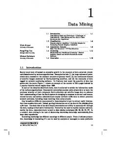
Figure 1.1: The Cuneane molecule does not have a unique encoding in Daylight’s published specification of Canonical Smiles [193]. Two representations are depicted here.

molecules. Molecules are structured objects which illustrate some of the problems of mining structured data very nicely. Let us consider the application of mining molecules in more detail. In recent years there have been large screening programs in which the activity of molecules has been tested with respect to aids inhibition, toxicity or mutagenicity. Chemists are interested in finding ‘structure activity relationships’ between molecules and activities, and databases can be used to gain more insights into these relationships. There are reasons to believe that substructures (‘fragments’) of molecules can be essential to the activity of molecules. However, there are many ways in which molecules can be encoded. One can choose a detailed level of description —the atomic level—, or more abstract levels in which properties of fragments that are known to be of importance (hydrogen donors, aromatic rings, . . .) are also incorporated in the data or the mining algorithm. In practice, mining molecules reduces to a repeated sequence of in silico experiments in which the researcher gradually tries to get an idea about the factors of importance, and tries to find the correct encoding in combination with the most interesting constraints. Already early in data mining research it was realized that this problem of molecule mining seems very well suited as a showcase for inductive database technology. Based on the algorithms described in this thesis, we developed a set of tools that allow chemists to analyze their data. To deal with structured data all kinds of problems have to be tackled that are almost trivially solved in attribute-value mining algorithms. While some operations on rows of attributes are very easily performed —for example, to determine if an attribute in a row has a certain value, is a trivial operation— in structured data the counterpart operations —for example, to determine if a molecule contains a certain fragment— are very complicated, both computationally and conceptually. Computationally, it is known that to determine whether a molecule contains a certain fragment is among the hardest problems that one can ask a computer to solve. For arbitrarily large molecules and fragments currently no algorithms are known that are guaranteed to find an answer within reasonable time. The conceptual difficulty of the fragment inclusion problem is illustrated by a paper of the Weilinger family in 1989. Weilinger, Weilinger and Weilinger are well-known in chemin-

6

1. Introduction

formatics for their development of SMILES, which is a representation language for chemical compounds [192]. To allow SMILES to be used in database indexing, they developed canonical SMILES in 1989, which, according to their claims, was a unique encoding for molecules that can be computed in polynomial time. Yet, this claim turns out to be false. We found that the cuneane molecule which is depicted in Figure 1.1 —a molecule which is not very common, but certainly chemically stable— does not have a unique representation in Canonical SMILES. The problem of this molecule is that all atoms have the same number of connections to other atoms, and that all neighboring atoms are of the same type. Yet, Canonical SMILES fails to note that some carbon (‘C’) atoms are part of a triangle, while others are not1 . From a computer scientist’s perspective the problems involved when mining molecules are very challenging: we are confronted with large datasets, large search spaces and hard computations to relate datasets and patterns. In this thesis we give much attention to these computational aspects. We develop mechanisms that work well on several structured databases, including molecular databases; however, we also devote much space to proving formally that our algorithms do not only work well in practice, but also perform the task that they are supposed to do.

1.3 Overview Many publications in recent years have studied the same problems as we have considered during our research. In most cases, these publications describe a new system that can be used to perform a well-defined data mining task ‘efficiently’. The disadvantage of such systembased publications is however that a good overview of how these systems relate to each other, is missing. Furthermore, relations to other research topics, such as complexity theory, have not been given much attention by most researchers either, in some cases perhaps even because the contribution of some papers would otherwise be recognized as rather small. In this thesis we set ourselves the ambitious goal of not only describing our own systems, but also of providing a more general overview of the research that has been going on in this field in recent years. An overall contribution of this thesis, also in comparison with our own previously published papers, is therefore that we try to build a theoretical framework in which not only our own algorithms, but also other algorithms can be fitted. Finally, we not only theoretically compare our systems to a large number of other systems, but also perform a broader set of experiments than has been published before. As a consequence, the thesis is organized as follows. In Chapter 2 we introduce the problem of frequent itemset mining. Frequent itemset mining is the simplest form of frequent pattern mining as it involves only one constraint and applies to single tables only. Many of the methods for constrained pattern mining are essentially extensions of approaches for mining frequent itemsets, and it is therefore most instructive to review these approaches first. In this chapter, we will see that generally two search orders are employed in frequent itemset mining: breadth-first and depth-first; further1 It is therefore not a surprise that the Daylight Tools, in which the Weilinger family implemented their algorithm, quietly do not use the canonical SMILES representation of 1989 any more.

1.3. Overview

7

more, there are two ways to evaluate constraints in databases: using additional datastructures such as occurrence sequences, or by recomputing occurrences of patterns in the data. In Chapter 3 we review the general problem of mining patterns under constraints. Most theoretical concepts that are of importance for future chapters are introduced in this chapter, among which relations (that describe how patterns relate to each other and to data), monotonic and anti-monotonic constraints (that can be used to prune the search space), refinement operators (that describe in which way the search space is traversed), and general frameworks in which constraint pattern mining algorithms can be fitted. We review a large set of existing algorithms for constrained pattern mining. Of importance in this chapter is the introduction of merge operators. We believe that the concept of a merge operator enables a more precise specification of many efficient pattern mining algorithms. One of the purposes of this chapter is to show that structured data causes a large set of additional problems, but that there also additional chances to combine several types of structures (for example, ordered and unordered) with each other. In Chapter 4 we treat our first type of structured data: the multi-relational databases. We define patterns in terms of first order logic and consider three possible relations between such patterns in multi-relational databases. Exploiting the existence of primary keys in many relational databases, we define the weak Object Identity relation between sets of first order logic atoms, and show that this relation has several desirable properties. We use this relation as an element of F, which is an algorithm for mining frequent atom sets more efficiently than other algorithms. Essential elements of this algorithm are discussed, such as its merge operator and its algorithm for evaluating patterns in the data. Also here an overview is provided comparing our work to other work in this field. Large parts of this work have been published in [144, 146, 147, 150]. In Chapter 5 we treat the second type of structured data: the rooted trees. We introduce several kinds of relations between rooted trees, provide refinement operators, merge operators, and give alternative evaluation strategies. A contribution in this chapter is a new refinement operator for traversing search spaces of unordered trees. We show how this refinement algorithm relates to a well-known enumeration algorithm for such search spaces. Furthermore, we introduce a new incremental algorithm for evaluating the subtree relation efficiently. All these elements are then evaluated, not only theoretically, but also experimentally. Of course, we compare our work extensively with other work. Parts of this work were published in [145, 37]. In Chapter 6 we extend approaches for mining trees to deal with the third type of structured data: the graphs. By searching first for trees, and then for graphs, we hope to obtain more efficient algorithms. Furthermore, some constraints, like a constraint on the smallest distance between nodes in a pattern, are more easily pushed in the mining process if we search for trees first. We repeat the exercise of providing refinement operators, merge operators and evaluation strategies. We compare our work thoroughly with other work. This chapter includes a discussion of the G algorithm for mining frequent subgraphs, which was first published in [151], and also presented in [148, 149]. Although in most chapters we give some experimental results, the most extensive experimental results are provided in Chapter 6. In this chapter we also reflect on some of the properties of other frequent pattern miners that we presented in the previous chapters, and we provide an even more detailed idea about the issues involved in obtaining frequent pattern

8

1. Introduction

mining algorithms of good performance. In Chapter 7 we return to the more general problem of mining correlated patterns. We show that correlated pattern mining is very closely related to the frequent pattern mining problem; in terms of inductive queries, we show that it can be solved by a combination of frequent pattern mining queries of which the results are postprocessed, thus providing an example of how inductive queries can be combined to obtain meaningful new queries. As a main contribution to existing work, we show that this approach extends even to correlated pattern mining in databases where there is a target class attribute with multiple values. This chapter was published in [152].

2

Frequent Itemset Mining

In this chapter we provide a brief review of frequent itemset mining research. First we introduce the problem of frequent itemset mining; then we discuss the details of the most wellknown algorithms: in chronological order we introduce the breadth-first, horizontal A algorithm, the vertical E algorithm and the depth-first FP-G algorithm, all of which are intended to solve the problem as efficiently as possible. Our aim is to introduce several concepts within their original setting of frequent itemset mining before extending them to structure mining in later chapters.

2.1 Introduction Frequent itemset mining has its roots in the analysis of transactional databases of supermarkets. Early in the nineties the introduction of bar code scanners and customer cards allowed supermarkets to start maintaining detailed databases. The natural question arose if there were ways to exploit this data. In 1993 Agrawal et al. [6] introduced itemset mining as a means of discovering knowledge in transactional supermarket data. Although since then itemset mining has been applied in many other application domains and for many other purposes —we will see examples later—, the terminology still reflects these historic roots. Itemset mining algorithms take as input a database of transactions. Each transaction consists of a set of items (also called a basket). In the supermarket application, a transaction may correspond to the products that have once been bought by one particular customer. A small example is given in Figure 2.1. Itemset mining algorithms have been designed as an aid in the discovery of associations between products. These association rules formalize observations such as all customers that buy broccoli and egg, also buy aubergine —at least, in our example database. Eventually, we wish to construct an algorithm which discovers such potentially surprising associations between products completely automatically.

10

2. Frequent Itemset Mining

Tid t1 t2 t3 t4 t5 t6 t7 t8 t9 t10

Itemset {broccoli} {egg} {aubergine, cheese} {aubergine, egg} {broccoli, cheese} {dill, egg} {cheese, dill, egg} {aubergine, broccoli, cheese} {aubergine, broccoli, egg} {aubergine, broccoli, cheese, egg}

Figure 2.1: A small example of an itemset database.

More formally, it is said that there is a set of items I = {i1 , . . . , in }, a finite set of transaction identifiers A and a database D ⊆ {(t, I)|t ∈ A, I ⊆ I} that contains exactly one itemset for each transaction identifier. An itemset with k items is called a k-itemset. Every transaction in the database can be identified through a transaction identifier (the Tid t), which makes sure that two customers that buy the same set of items are still treated as different customers. Equivalently, one could also define D as a multiset; in that case the transaction identifier is not necessary. The set of occurrences of an itemset I, which is denoted by occD (I), is defined by1 : occD (I) = {t | (t, I ′ ) ∈ D, I ⊆ I ′ }. The support of an itemset I, which is denoted as supportD (I), is defined as: supportD (I) = |occD (I)| . In the example database we have that supportD ({broccoli, egg}) = |{t9 , t10 }| = 2. We will omit D in the notation if this is clear from the context. An association rule is a rule of the form I1 → I2 , where I1 , I2 ⊆ I. The support of an association rule, support(I1 → I2 ), is defined by support(I1 → I2 ) = support(I1 ∪ I2 ). The confidence of an association rule is defined by confidence(I1 → I2 ) = 1 Sometimes

ogy.

support(I1 ∪ I2 ) , support(I1 )

the set of occurrences is also called the cover or the support set, but we will never use that terminol-

2.2. Frequent Itemset Mining Principles

11

where it is required that support(I1 ) , 0. In the example the confidence of the association rule {broccoli, egg} → {aubergine} is confidence({broccoli, egg} → {aubergine}) =

support({aubergine, broccoli, egg}) 2 = = 1. support({broccoli, egg}) 2

The idea behind association rule mining is that rules with both a high support and a high confidence are very likely to reflect an association of interest, and one would therefore be interested in finding all such rules. The example rule has the highest confidence possible and may therefore be of interest. In the remainder of this chapter, we review some of the basics in itemset mining research. In section 2.2 we provide the basic principles of frequent itemset mining. After an intermezzo in section 2.3, in which we introduce notation, we review the most important algorithms for mining frequent itemsets: A (section 2.4), E (section 2.5) and FP-G (section 2.6). Section 2.7 concludes.

2.2 Frequent Itemset Mining Principles Although the idea of finding all itemsets with high support may sound attractive, several problems have to be addressed to make frequent itemset mining successful. The foremost problem is the large number of possible rules. For |I| items there are 2|I| possible itemsets. From each of these itemsets an exponential number of rules can be obtained. In most cases it will therefore be intractable to consider all itemsets. The essential idea that was presented in 1993 was to restrict the search only to those itemsets for which the support is higher than a predefined threshold value, the so-called minimum support. Initially such itemsets with high support were called large itemsets [6, 8, 7]. However, this term caused confusion as most people felt that ‘large’ referred to the number of items in an itemset, and did not reflect support. In 1995, therefore, the terminology was changed and the term frequent itemset was introduced [176]. An itemset I is therefore now called a frequent itemset iff: support(I) ≥ minsup, for a predefined threshold value minsup. An itemset is large if it has many items. The set of all frequent itemsets in the example of Figure 2.1 is illustrated in Figure 2.2. In this figure the products have been abbreviated with their first letter. The lines visualize the subset relation: a line is drawn between two itemsets I1 and I2 iff I1 ⊂ I2 and |I2 | = |I1 | + 1. Such a figure is usually called a Hasse diagram. An important property that will always hold for itemsets is the following: if I1 ⊆ I2 then support(I1 ) ≥ support(I2 ).

(2.1)

This property follows from the fact that every transaction that contains I2 also contains I1 . In our example, support({egg}) = |{t2 , t4 , t6 , t7 , t9 , t10 }| = 6 ≥ support({broccoli, egg}) = |{t9 , t10 }| = 2.

12

2. Frequent Itemset Mining ∅

{A}

{B}

{C}

{D}

{E}

{A, B}

{A,C}

{A, D}

{A, E}

{B,C}

{B, D}

{B, E}

{C, D}

{C, E}

{D, E}

{A, B,C}

{A, B, D}

{A, B, E}

{A,C, D}

{A,C, E}

{A, D, E}

{B,C, D}

{B,C, E}

{B, D, E}

{C, D, E}

{A, B,C, D}

{A, B,C, E}

{A, B, D, E}

{A,C, D, E}

{B,C, D, E}

{A, B,C, D, E}

Figure 2.2: A visualization of the search space for the database of Figure 2.1; frequent itemsets for minsup = 2 are highlighted.

A consequence of this property is that if support(I) < minsup then for all I ′ ⊇ I : support(I ′ ) ≤ support(I) < minsup. When we are searching for frequent itemsets this observation means that we do not have to consider all supersets of an itemset that is infrequent, as one can easily see that every superset is also infrequent. Therefore, if the search is performed such that itemsets are considered incrementally, itemsets can be pruned from the search space by applying this property. Although the size of the search space remains of size 2|I| theoretically, the seducing challenge posed by frequent itemset mining is to implement algorithms that traverse the search space such that the search becomes tractable in practice. As the extent to which this is possible clearly depends on the predefined threshold minsup, part of the challenge is to define algorithms that still work on as low supports as possible. Many such algorithms have been developed; a brief overview of the most important algorithms will be given in later sections.

2.3 Orders and Sequences Before turning to the introduction of the frequent itemset mining algorithms, however, we need to introduce some formal notation. We will come back to these definitions in more detail in the next chapter. Definition 2.1 (Orders) Given is a set X and a binary relation R which is a subset of X × X.

We call relation R

2.3. Orders and Sequences

13

1. reflexive if for all x ∈ X, xRx holds. 2. transitive if for all x, y, z ∈ X, xRy and yRz imply that xRz. 3. antisymmetric if for all x, y ∈ X, xRy and yRx imply that x = y. 4. total if for all x, y ∈ X, either xRy or yRx holds (or both). Relation R is called a quasi-order if R is reflexive and transitive. If a quasi-order R is antisymmetric, this relation R is called a partial order. If a partial order R is total, the relation is called a total order. We denote orders using symbols like . If x y and x , y this is denoted by x ≻ y. If the order is clear from the context x ≡ y is a shorthand for x y and y x. Furthermore, for relations denoted by x y, we will also use y x as an alternative notation if this is more convenient. As an example, on the domain of natural numbers (X = N) the traditional comparison between numbers (≥) is a total order, as for every i ∈ N, i ≥ i holds; for all integers i, j and k, i ≥ j and j ≥ k imply that i ≥ k; if i ≥ j and j ≥ i, then i = j; for all integers i, j ∈ N it holds that i ≥ j or j ≥ i, or both. Definition 2.2 (Sequences) Let X be a domain.

1. X∗ denotes the set of finite sequences over X. A typical sequence is denoted by S , S 1 , S 2, . . . 2. ǫ denotes the empty sequence; 3. |S | denotes the length of sequence S ; 4. S [k] denotes the kth element of sequence S , if 1 ≤ k ≤ |S |, and is undefined otherwise; 5. S 1 • S 2 denotes the concatenation of sequences S 1 and S 2 ; 6. S • x denotes the concatenation of element x ∈ X after sequence S ; 7. S [k . . . ℓ] denotes the subsequence of sequence S consisting of the consecutive elements S [k], S [k + 1], . . . , S [ℓ], if 1 ≤ k ≤ ℓ ≤ |S |, and is undefined otherwise. 8. S −1 denotes the reverse of sequence S ; 9. prefixk (S ) denotes the prefix of length k of sequence S , if 0 ≤ k ≤ |S |, or denotes the prefix of length |S | + k if −|S | ≤ k < 0, and is undefined otherwise. 10. prefix(S ) denotes the prefix of length (|S | − 1) of a non-empty sequence S ; 11. S 1 ⊓ S 2 denotes the largest prefix that sequences S 1 and S 2 have in common; 12. suffixk (S ) denotes the suffix of length k of sequence S , if 0 ≤ k ≤ |S |, and is undefined otherwise. 13. suffix(S ) denotes the suffix of length (|S | − 1) of a non-empty sequence S ;

14


14. first(S ) and last(S ) denote the first and the last element of a sequence S , if |S | ≥ 1, and are undefined otherwise. 15. S 1 /S 2 is the sequence S which satisfies S 1 = S 2 • S , when such a sequence can be found, and is undefined otherwise; 16. Rlex denotes the lexicographical order on sequences, where the elements in the sequence are ordered by relation R; 17. set(S ) denotes the set X = {S [k] | 1 ≤ k ≤ |S |} for sequence S ; 18. x ∈ S is a shorthand notation for x ∈ set(S ). As examples consider the sequences S 1 =ABC and S 2 =AB. According to our definitions the following statements hold: prefix2 (S 1 ) = AB, suffix2 (S 1 ) = BC, S 1 • S 2 = ABCAB, (S 1 /S 2 ) = C, first(S 1 ) = A, S 1 [3] = C. If the domain X = {A, B,C} is totally ordered as follows: C B A (alphabetical), we have that S 1 lex S 2 . For itemsets we furthermore introduce the following notation: given an itemset I ⊆ I and an order > on the items in I, seq> (I)

denotes the sequence S = i1 i2 . . . in that contains all elements of set I exactly once, such that ik+1 > ik for all 1 ≤ k ≤ n − 1. Thus, operator seq(I) can be used to transform itemsets into sequences in a unique way. Given the alphabetic order on X = {A, B,C}, we have that seq({A, B,C}) = ABC. Usually it would be cumbersome to write down all conversions between sets and sequences. Therefore, if the order is clear from the context, we also use implicit conversions. We assume that the order is alphabetical in most of our examples. In that case, for example, we will also write that prefix({A, B}) = A, although strictly speaking we would have to write that prefix(seq ({A, B})) = A for an alphabetical order .

2.4 A The most well-known frequent itemset mining algorithm is the A algorithm. This algorithm was independently proposed in the summer of 1994 by both American [8] and Finnish [126] researchers. A joint paper about the algorithm was published in 1996 [7]. The algorithm is based on the idea of maximizing the use of equation (2.1), which was therefore called the a priori property by these authors. An overview of the algorithm is given in Figure 2.3. The A algorithm traverses the itemsets strictly increasing in size, and uses a generateand-test approach. In an initial pass through the database it is determined which single items are frequent. Then repeatedly candidate itemsets are generated and their frequency is determined. More details of these two phases are discussed in the next sections.

2.4. A

15

(1) A(D): (2) F1 := { frequent itemsets with one item}; (3) order the items; (4) k := 2; (5) while Fk−1 , ∅ do (6) Ck := A-G(Fk−1 ); (7) for all (t, I) ∈ D do (8) for all candidates C ∈ Ck for which C ⊆ I do (9) support(C) := support(C)+1; (10) Fk := {C ∈ Ck | support(C) ≥ minsup}; (11) k := k + 1; (12) return ∪k Fk ; Figure 2.3: The A algorithm.

A-G The input of A-G is the set of all frequent (k − 1)-itemsets, Fk−1 . Although items are initially unordered, before starting the algorithm an order is imposed upon them. We assume an alphabetical order in our examples. The candidate generation procedure consists of two phases. In the first phase, all pairs of item sequences C1 and C2 ∈ Fk−1 with prefix(C1 ) = prefix(C2 ) and last(C1 ) < last(C2 ) are combined to obtain itemsets with k items. In the example itemsets {A, B,C} and {A, B, E} ∈ F3 , whose sequences ABC and ABE share common 2-prefix AB, are combined into {A, B,C, E}. Itemsets {B,C} and {C, E} are not combined, as they do not have a common 1-prefix. Every itemset that is generated in this way has at least two frequent subsets. To make sure that all subsets are frequent, a second step is performed. Given a candidate C ∈ Ck , the following check is computed: is for all i ∈ C the set C\i an element of Fk−1 ?

(2.2)

As we noted that candidates generated in the first phase already have two frequent subsets, this test is equivalent to the following more efficient test: is for all i ∈ prefixk−2 (seq(C)) the set C\i an element of Fk−1 ?

(2.3)

In the example database this means that for the preliminary candidate {A, B,C, E} it is checked whether {{B,C, E}, {A,C, E}} ⊆ F3 . As {B,C, E} < F3 we can use the a priory property to conclude that {A, B,C, E} can never be part of F4 . In the second phase of candidate generation such candidates are therefore removed from Ck . To implement the generation of candidates, in [8, 7] the use of a hash tree was proposed. Here we will discuss a variation of this same idea, the (prefix) trie [25]2 . An illustration of a trie for a set of frequent itemsets is given in Figure 2.4. The main purpose of the trie is to allow for a quick search for a sequence S , by performing the following procedure: 2 Trie

stands for word retrieval tree [196].

16


A

B

C

E

C

B

C

E

D

E

E

Figure 2.4: A prefix trie of F2 for the database of Figure 2.1.

A

B

C

E

B

C

C

E

E

Figure 2.5: A trie of C3 for the database of Figure 2.1.

1. set i to 1, and let v be the root of the trie; 2. search for S [i] in node v; 3. let v be the child node associated to S [i] in the trie, increase i with 1, and go to 2. Thus, every node in the trie has a table in which items are stored. To allow for a quick search the table can be implemented as a hash index [8, 7] or as a sorted array [25]. It is clear that if we search for an item sequence in a trie, one unique path through the trie is traversed. If we search for a k-sequence in a prefix trie of k-itemsets, we end our traversal in one of the leafs. Furthermore, itemsets with common (k − 1)-prefixes will always end up in the same leaf. Indeed, in Figure 2.5, the prefix AB has corresponding node C E , which represents sequences ABC and ABE. The task of candidate generation can be formulated as a problem of creating a ‘new’ prefix trie from an ‘old’ prefix trie. Figure 2.5 illustrates the prefix trie that is created from the trie in Figure 2.4. The structure of the prefix trie can be used in several ways during candidate generation. First, we saw that two k-itemsets with a common (k − 1)-prefix are represented in the same node. In phase one of the generation all candidates can therefore be obtained by combining itemsets within one node. In our running example, frequent itemset {B,C} ∈ F2 is stored in trie node C E (Figure 2.4). It is joined only with itemset {B, E}, which is stored in the same node. This operation yields the rightmost leaf of the trie in Figure 2.5. Second, to compute the pruning test of equation (2.2), repeatedly the existence of (k − 1)itemsets in Fk−1 has to be determined. This search is performed efficiently by searching for

2.4. A

17

these sets in the trie of Fk−1 . We already noted that items should be ordered totally before running the algorithm. Although one could choose this order arbitrarily (for example, alphabetically), the order may have consequences on the efficiency of the total candidate generation. It has therefore been proposed to determine a ‘good’ order heuristically before starting the main loop of A. One such order could be determined using the supports of the individual items. In our example items A, B and C have support 5, item D has support 2 and item E has support 6. First, consider an order of decreasing support, E < A < B < C < D. In that case itemsets {C, E} and {D, E} would be represented by sequences EC and ED, which would be joined into candidate ECD. This candidate is removed again in the second phase. What we see is that itemsets that are contained in one trie node are relatively infrequent, and that therefore their join is very likely to be infrequent too. Overall, the join is therefore not very efficient. However, in the order of increasing support, D < A < B < C < E, we would have that {C, E} and {D, E} are represented by sequences CE and DE, which are not joined. As in general this ascending order ‘pushes’ frequent items to the ‘back’ of item sequences, it is more likely that two frequent itemsets with common prefixes will generate a frequent itemset when joined. In general it has therefore been claimed that for the candidate generation of A it is favorable to consider items in ascending order of support [25]. One should remember, however, that this is nothing more than a heuristic [104]. Candidate counting

Once a set of candidates has been built the real frequencies of these candidates have to be determined. In the A algorithm this operation is performed by scanning the entire database. To find out which candidates are included in a transaction, the prefix trie can be exploited again. For this purpose the itemsets in the leafs3 of the trie are extended with count fields, in which the frequencies of the itemsets are stored. The pseudocode of Figure 2.6 illustrates the counting procedure at a high level, without optimizations. Line (2) essentially determines the intersection between items in the trie node and items in the transaction. There are many ways to implement this intersection, among others: • If both the transaction and the table are stored as sorted arrays, the computation comes down to traversing both arrays to obtain the intersection [25]. • If the transaction is stored in a binary array such that the ith bit is 1 iff item i is included in the transaction, then one only has to traverse the candidate array and to check the status of the corresponding bit in the binary array [159]. • If the transaction is stored as a sorted array, and the candidates are stored in a hash table, then one has to traverse the transaction and to check the presence of the transaction in the hash table [8, 7]. Several other optimizations can be applied. For more details, we refer the reader to the original publications. 3 In practice many algorithms also store supports in other nodes; most of these algorithms do not repeatedly build new tries, but modify existing datastructures in memory.

18


(1) Apriori-Count-Rec(Transaction Itemset I, trie node v): (2) for all i ∈ I stored in trie node v do (3) if i has an associated child v′ in v then (4) A-C-R(I, v′ ); (5) else (6) count(v, i) := count(v, i)+1; (1) Apriori-Count(Transaction (t, I), Prefix Trie PT): (2) A-C-R(I, root(PT))

Figure 2.6: An algorithm for counting candidates in a transaction.

Item Aubergine Broccoli Cheese Dill Egg

Tids {t3 , t4 , t8 , t9 , t10 } {t1 , t5 , t8 , t9 , t10 } {t3 , t5 , t7 , t8 , t10 } {t6 , t7 } {t2 , t4 , t6 , t7 , t9 , t10 }

Figure 2.7: The vertical representation of the itemset database in Figure 2.1.

2.5 E As we saw in the previous section, the A algorithm takes as input a database which is repeatedly scanned to count candidates. The database itself is not modified by the algorithm. Early in the nineties, this approach was necessary as the amount of main memory in computers was relatively limited, and most databases therefore had to be kept on disk. In the A algorithm it is possible to independently process blocks of transactions, thus limiting the amount of main memory required, while additional storage space is only required for maintaining the candidates. With the increase of hard disk capacities and main memory sizes, researchers started to investigate approaches that demand more storage space. One such approach was based on the idea of storing databases vertically instead of horizontally, and was presented by Zaki et al. in 1997 [207]. Figure 2.7 illustrates the vertical representation of our example database. For each item i in the database, in the vertical representation the set occ(i) is stored. The vertical mining approach now uses the observation that in A a k-itemset (with k > 1) is always generated by joining two other itemsets, and it is always possible to determine the occurrences of a new itemset by computing the intersection between the occurrences of the generating itemsets. In our example, we have that

2.5. E

19

occ({A, B,C}) = occ({A, B}) ∩ occ({A,C}) = {t8 , t9 , t10 } ∩ {t3 , t8 , t10 } = {t8 , t10 }. Also in general it can easily be seen that occ({i1 , i2 , . . . , in }) = occ({i1 , i2 , . . . , in−1 } ∪ {i1 , i2 , . . . in−2 , in }) = occ({i1 , i2 , . . . , in−1 }) ∩ occ({i1 , i2 , . . . , in−2 , in }) is always true. If we store the occurrence sets not only of single items, but also of larger itemsets, support could always be computed by intersecting occurrence sets. Clearly, this approach requires more storage as all occurrences have to be stored somewhere. Several studies have attempted to reduce this burden. We will discuss several of them. Encoding issues

When dealing with occurrence sets, an important factor is the representation that is chosen to store such sets. There are many possibilities: 1. store occurrence sets in arrays such that each array element contains the identifier of a transaction included in the sets [207, 205]; alternatively, one could choose to store the elements in a list or more elaborate data structures; 2. store occurrence sets in arrays such that each element contains the identifier of a transaction that is not included in the sequence [205]; note that the original sequence can easily be reconstructed by listing ‘missing identifiers’ if transactions are numbered consecutively; 3. store occurrence sets in binary arrays such that the ith element of the array is 1 iff the ith transaction is part of the sequence [207], and 0 otherwise; 4. use elaborate compression schemes to store bit arrays, such as variations of run length encoding [174]. For future reference we elaborate here on of the second option. One of the major issues with occurrence sets is their potentially large size in the case of dense datasets. If an item is present in almost all transactions, its occurrence set will be very large; also, in later stages, the occurrences of itemsets with and without this item will not differ very much. Such large occurrence sets are a problem as they increase both the computation time and the amount of storage required. Taking this problem into account, Zaki et al. [205] proposed the use of diffsets. While an occurrence set contains the transactions that support an itemset, in a diffset the identifiers are stored of transactions that do not support a given itemset. More precisely, given an itemset sequence I, it is defined that diff (I) = occ (prefix (I)) \occ (I) . In our example, we have that diff(ABC) = occ(AB)\occ(ABC) = {t8 , t9 , t10 }\{t8 , t10 } = {t9 }.

(2.4)

20


Note that the diffset does not contain the identifiers of all transactions that do not support an itemset (as implied in option 2. above), but that the diffset only stores the difference in comparison with its prefix itemset. Furthermore note that it follows that occ (I) = occ (prefix (I)) \diff (I) ,

(2.5)

as we know that occ (I) ⊆ occ (prefix (I)). The support of an itemset can therefore be determined using support (I) = support (prefix (I)) − |diff (I)| . The computation of diffsets and supports can now proceed as follows. Assume that given is a set of k-itemset sequences with common (k − 1)-prefixes, and that we have the diffset and support of each itemset. Then for two itemsets I1 ≤ I2 , the diffset of I1 ∪ I2 is diff(I1 ∪ I2 ) = diff (I2 ) \diff (I1 ) , as diff(I1 ∪ I2 ) = occ (prefix (I1 ∪ I2 )) \occ (I1 ∪ I2 ) = occ (I1 ) \ (occ (I1 ) ∩ occ (I2 )) = occ (I1 ) \occ (I2 ) = (occ (prefix (I1 )) \diff (I1 )) \ (occ (prefix (I2 )) \diff (I2 )) = diff (I2 ) \diff (I1 ) .

(Definition, Eq. 2.4) (prefix (I1 ∪ I2 ) = I1 ) (Set theory) (Eq. 2.5)

In the last step we use set theory and the facts that the sets diff(I1 ) and diff(I2 ) are subsets of occ (prefix(I1 )) = occ (prefix(I2 )). The support of I1 ∪ I2 is determined by support (I1 ∪ I2 ) = support (I1 ) − |diff (I1 ∪ I2 )| . Although it is possible to perform the entire search using diffsets or occurrence sets, the two approaches can also be combined. We saw that diff(I1 ∪ I2 ) = occ(I1 )\occ(I2 ): thus, one can also choose to switch from occurrence sets to diffsets during the search. To switch the other way around is more complicated and possibly undesirable. As the diffset only stores the difference with the largest proper prefix, the diffset of each prefix is required to recompute the occurrence set: occ(i1 i2 . . . ik ik+1 . . . in ) = occ(i1 i2 . . . ik )\diff(i1 i2 . . . ik+1 )\ · · · \diff(i1 i2 . . . in ), where i1 i2 . . . ik is the largest prefix for which an occurrence set is known. Clearly, to switch from diffsets to occurrence sets one has to store large numbers of occurrence sets and diffsets, also for very small itemsets. Depth-first search

Already early in frequent itemset research it was noticed that there are also recursive ways to find all frequent itemsets. The basic observation is simple: given an order R on items I and one frequent item i ∈ I, from a given database D one can build a new database that:

2.5. E

21

(1) Depth-First-Search(Itemset I, Database D): (2) F := F ∪ {I}; (3) determine an order R on the items in D; (4) for all items i occurring in D do (5) Create from D projected database Di , containing: - only transactions that in D contain i; (6) - only frequent items in Di that are higher than i in R. (7) (8) Depth-First-Search(I ∪ {i},Di ); Figure 2.8: A high-level overview of a depth-first frequent itemset mining algorithm.

• consists of only those transactions that contain item i; • consists of only those items i′ that are higher than i, according to R. Such a database is called a projected database. If i′ is a frequent item in the projected database, we know that {i, i′ } is a frequent itemset in the original database. By recursively projecting projected databases longer frequent itemsets can be found. The A property is applied implicitly by projecting only on frequent items and not on infrequent ones. A general outline of such a procedure is given in Figure 2.8. We will first consider the case that the database is stored vertically using occurrence sets, as given in Figure 2.7. The Depth-First-Search algorithm is called with itemset ∅ and the collection of all occurrence sets as parameter. After adding ∅ to F the Depth-First-Search algorithm orders the items in the database, for example, in ascending order of support: D < A < B < C < E. Each of these items is then considered in isolation. We will consider item A as an example. The projected database DA should contain the following information: occDA ({B}) = occD ({A, B}) = occD ({A}) ∩ occD ({B}) = {t8 , t9 , t10 }; occDA ({C}) = occD ({A,C}) = occD ({A}) ∩ occD ({C}) = {t3 , t8 , t10 }; occDA ({E}) = occD ({A, E}) = occD ({A}) ∩ occD ({E}) = {t4 , t9 , t10 }. Those sets which turn out to be infrequent are not included in DA ; as in our example all itemsets are frequent, no previously computed occurrence sets are deleted. The Depth-First-Search procedure is recursively called for this projected database. This time {A} is added to F at the start of the procedure. The items in DA are sorted again, B < C < E; each is considered in turn again, for example B. Again the database is projected: occDAB ({C}) = occDA ({B,C}) = occDA ({B}) ∩ occDA ({C}) = occD ({A, B}) ∩ occD ({A,C}) = {t8 , t10 }; occDAB ({E}) = occDA ({B, E}) = occDA ({B}) ∩ occDA ({E}) = occD ({A, B}) ∩ occD ({A, E}) = {t9 , t10 }.

22


For DAB Depth-First-Search is called recursively again. Within this call, {A, B} is added to F , the items in DAB are ordered, C < E, and DAB is projected on item C: occDABC ({E}) = occDAB ({C, E}) = {t10 }. As item E is not frequent within DABC , this occurrence list is removed. One last time DepthFirst-Search is called with an empty database. This call adds {A, B,C} to F , but does not recurse further. Also in general it is easily seen that this procedure is correct and adds each frequent itemset to F exactly once. We believe that the key to an easy understanding is the concept of a ‘projected database’. There are however many other ways in which one could think of depth-first algorithms. We wish to mention some of the links with the original A algorithm: • In depth-first algorithms the items are often reordered during the search, while in A the order is fixed once. In A a reordering would be impractical as it would make the search in the prefix trie more complicated, but in depth-first algorithms this is much less of a problem. • Both algorithms extensively use the fact that is very easy to organize itemsets in a tree: A stores itemsets in a tree datastructure, while Depth-First-Search organizes the search in a tree. Both trees are closely related to each other. For example, A stores itemsets with a common prefix in one trie node; Depth-First-Search uses itemsets with a common prefix to build a projected database. • There memory requirements of A and depth-first algorithms are different; which one is more efficient, depends on the data. For example, in our example A stores the following collection of frequent itemsets in a trie of itemsets of size 3: {A}, {B}, {C}, {D}, {A, B}, {A,C}, {A, E}, {B,C}, {B, E}, {C, E}, {D, E}; itemsets {C} and {D} are implicitly stored in the trie as they are part of the prefix of {C, E} and {D, E}. The following 3-itemsets are stored later: {A}, {A, B}, {A, B,C}, {A, B, E} While considering the projected database of item A we saw that the depth-first algorithm has the following frequent itemsets in memory: {A}, {B}, {C}, {E}, {A, B}, {A,C}, {A, E}. Itemsets {{A, B}, {A,C}, {A, E}} are part of the projected database; also still in memory are itemsets {{B}, {C}, {E}} as the procedure will backtrack to these sets later. While considering the projected database for AB the following itemsets are in memory {{{A}, {B}, {C}, {E}, {A, B}, {A,C}, {A, E}, {A, B,C}, {A, B, E}}. It has been claimed that in practice depth-first algorithms require less memory than breadth-first algorithms when using occurrence sets.

2.6. FP-G

23

• An issue of debate is whether depth-first algorithms perform ‘candidate generation’ or not. A first generates a set of itemsets, and then computes the support of these generated itemsets. For the occurrence set based algorithm one can surely argue that it also generates candidates: all pairs of items in the projected databases are joined just like in A; the supports of the resulting itemsets are determined afterwards by intersecting occurrence sets. However, as we will see in the next section, it has also been claimed that some depth-first algorithms do not perform candidate generation.

2.6 FP-G An important next step in the development of depth-first algorithms was the introduction in 2000 of the FP-G algorithm by Han et al. [77]. We will briefly discuss it here for the sake of completeness. Essential to FP-G is its datastructure for storing (projected) databases: instead of storing occurrence sets, FP-G uses a prefix trie to store the transactions. To this purpose, each field of the trie is extended with additional information: • the number of transactions that has been sorted down this field; • a pointer to a field in another trie node. The additional pointers are used to link together all fields that contain the same item. Pointers to the starts of these item lists are stored in a header table. The trie is constructed in several steps. In an initial pass the supports of the items in the original database are determined. The frequent items are sorted in descending order. Then, in a second pass, each transaction is sorted down an initially empty trie. Here, each transaction is represented by the sequence of items in support descending order. The descending order is a heuristic that attempts to make sure that the tree is as compact as possible. An example of the resulting FP-Tree is given in Figure 2.9. In comparison with the vertical database representation, the FP-Tree abstracts from the original transaction identifiers and obtains a more compact representation of identical transactions. The projection of an FP-Tree on a certain item is performed in two phases of computation. Each of these phases consists of a traversal of the corresponding item list. Each element in the item list is the end of a path that starts in the root of the tree. Each path corresponds to transactions containing the projecting item. In the first phase for each item on each of these paths the frequency is determined within the set of transactions represented by the paths. It can be shown that this can be accomplished by only considering the count fields within the FP-Tree. At the end of this phase, we know the supports of all items that are going to be part of the new projected database. Then, in the second phase, the new FP-Tree is actually built. Again, only transactions contained in the item list are considered, and of these transactions only the items ‘above’ the item list, which are the items with higher support in the current projected database. When adding the projected transactions to the new trie, the items are ordered in support descending order. This order was determined in the first phase.

24


E 6

E A B C D

A 3

B 2

C 1

D 1

D 1

A 2

B 1

B 2

C 1

C 1

C 1

Header table

C 1 Figure 2.9: An FP-Tree for the database of Figure 2.1.

It has been claimed that the FP-Tree is a very compact representation for many practical databases and that its construction procedure is very efficient [77]. Also independent studies have concluded that FP-G is among the most efficient algorithms, both in terms of memory requirements as in terms of runtimes [76]. The key source of efficiency seems to be the efficient compact representation, which abstracts from transaction identifiers. Several variants of the algorithm, all of which use this representation, perform consistently very good [76]. One can easily see that there are many similarities between E and FP-G. Both algorithms use a depth-first procedure and recursively project databases. At first sight it may seem that E and FP-G use different item orders, but this is not the case. FP-G sorts the items in support descending to obtain compact FP-Trees. Next, the projection procedure of FP-G includes all items in the projected database that are lower than the item that is used to project. With the descending support order these are exactly the items that have higher supports in the projected database, just like in E. A matter of taste is whether FP-G performs candidate generation or not. The authors of FP-G have explicitly titled their work as a method for mining frequent patterns without candidate generation [77]. The name of the algorithm —Frequent Pattern Growth— is also intended to reflect this. We believe that one might as well reason differently: during the first phase of the construction of FP-Trees in FP-G the supports of several items are determined in a projected database. This implies that, just like in E, all these items are considered to be candidate extensions; indeed, one has to allocate memory at some time to maintain the support counters for these candidates. Be it in an array or in a hash structure: by allocating memory one initializes these items as candidates, for which one is going to compute the support. Due to a lower amount of pruning, this number of candidates can even

2.7. Conclusions

25

be larger than in A (consider a database that contains one transaction with all items). The main difference between E and FP-G with respect to candidate generation is that E intersects the sets of any pair of items, while FP-G will only combine pairs of items that are found together in at least one transaction. It is only a matter of taste whether one considers this dynamic way of allocating counters candidate generation or not.

2.7 Conclusions After introducting the problem of frequent itemset mining, we have reviewed several algorithms to solve this problem. In terms of search strategy we subdivided these algorithms into two classes: the A breadth-first algorithm and the depth-first algorithms, among which FP-G and variants of E. The breadth-first algorithms have a generate-and-test approach and try to minimize the number of passes over the original database. The depth-first algorithms, on the other hand, build intermediate representations of the database to speed-up the search. We have seen two such representations: the vertical occurrence set representation and the FP-Tree. Although the algorithms are different in many aspects, they also share essential properties. In some way they all use the A property to restrict the search space. Equally important is however the low complexity of organizing itemsets into prefix trees. All algorithms either store itemsets in a prefix tree or perform a search that is organized according to prefixes. This makes it possible to easily find all frequent itemsets without duplicates. Although the observation seemed of little importance, it proved of vital importance that we could easily transform itemsets into item sequences just by sorting the items in no matter what order.

3

Theory of Inductive Databases

We provide an overview of the concepts that are of importance to constrained mining algorithms, including refinement operators, lattices, monotonic constraints and anti-monotonic constraints, and give an overview of constrained pattern mining algorithms, among which depth-first and breadth-first algorithms. For an efficient search we determine that refinement operators are of importance. We introduce the concepts of merge operators and suboptimal refinement operators, and show that for some types of structures depth-first mining with merge operators is difficult. Throughout the whole chapter we have a focus on patterns in general; our purpose is to demonstrate some of the difficulties of general pattern mining. We use frequent sequence mining as an example.

3.1 Introduction In the first chapter we introduced the idea of inductive databases and the challenges of mining complex structures. In this chapter we will introduce the formal concepts that are of importance to such inductive databases. As an inductive database has to search through a search space, it is of importance to have an algorithm that determines how new nodes in the search tree are generated. This concept is formalized through the refinement operator in section 3.2. We identify which properties of refinement operators are of importance in inductive databases. One of these properties is that of optimality. If a refinement operator is optimal this guarantees that each pattern in a search space is considered at most once by the algorithm. For many pattern domains optimal refinement turns out to be hard to achieve; to deal with these issues, we relax the definition of optimality to suboptimality. If the search space is large, we have to define mechanisms to limit the size of the search space. Typically, such a limitation can be obtained by applying constraints. We review possible constraints in section 3.4, and show how these constraints interact with the refinement operator. One of the most important constraints is the minimum frequency constraint which

28

3. Theory of Inductive Databases

we saw in the previous chapter. We will show that it can be hard to define this constraint in a usable way. Even if the search space is constrained, and it is computationally feasible to search it entirely, the set of results can be too large to be inspected manually. Section 3.5 provides an overview of condensed representations that have been proposed to summarize the results of inductive queries. We show that these representations extend to any kind of structures. From an algorithmic point of view, refinement operators are sufficient to traverse a search space. We saw in the previous chapter that there are two popular search orders: depth-first and breadth-first. In the case of itemset mining candidates are generated by joining itemsets with common prefixes. Also in algorithms for other pattern domains it can be useful to generate candidates through joins, as this may allow us to force the constraints more thoroughly. In section 3.6 we introduce the concept of merge operators to formalize this idea. Many algorithms have been proposed to mine under constraints. Some of these approaches extend to all pattern domains, others do not. Section 3.7 provides an overview of constrained pattern mining algorithms, and discusses to what extent these pattern mining algorithms can be applied to more general domains than the most studied domain of itemset mining. In this chapter we frequently use the problem of mining subsequences to illustrate the issues of mining under constraints. An overview of frequent sequence mining algorithms is provided in section 3.8 for the sake of completeness. In section 3.9 we conclude.

3.2 Searching through Space Intuitively, for a given database D we are searching within a certain pattern space X for a set of patterns X ⊆ X that satisfies constraints as defined by the user. Depending on the kind of constraints, the solution to this search may or may not be unique. In this thesis we mainly consider problems of the following kind: find all patterns x ∈ X for which q(x) = true, where q is a (deterministic) boolean function that returns true only for patterns that satisfy the constraint q; this function is the inductive query that is posed to the database, as introduced in Chapter 1. As we are studying the analysis of data in this thesis, the inductive query q is assumed to be based on the database D in some way. Note that within this setup there are only unary constraints on the patterns, and no higher dimensional constraints. As a consequence, the result of the inductive query is straightforwardly uniquely defined. We will come back to different possibilities in later chapters. Let us cast the frequent itemset mining problem into this framework. The search space of frequent itemset mining consists of all subsets of a set of items I, so X = 2I . As constraint we have that q(I) := true iff supportD (I) ≥ minsup. The database consists of transactions of itemsets. To find all patterns that satisfy constraints, a systematic search has to be performed. There are many kinds of systematic search, among others: breadth-first search, depth-first search, or hybrids of these search methods. Although different from many perspectives, all these search

3.2. Searching through Space

29

methods require a mechanism that determines for given (sets of) patterns which patterns to consider next. We saw in the previous chapter that frequent itemset mining algorithms use a procedure in which itemsets are joined with each other under certain constraints. For general patterns such a procedure may be hard to define straightforwardly. We will therefore start our discussion with the most basic procedure that can be used to traverse a search space: the refinement operator. There is a strong relation between refinement operators and more complicated mechanisms for generating candidates, as we will see in a later section. Definition 3.1 Let X be a domain of structures, and let X ⊆ X be a finite subset.

• A refinement operator is a total function ρ : X → 2X ; • A refinement operator ρ is (locally) finite if for every x ∈ X, ρ(x) is finite. Unless stated otherwise, we assume that refinement operators are locally finite. • ρn (x) denotes the n−step refinement of some structure x ∈ X: ( ρ(x) if n = 1; n ρ (x) = {z ∈ ρ(y) | y ∈ ρn−1 (x)} otherwise. • ρ∗ (x) denotes the set ρ∗ (x) = {x} ∪ ρ(x) ∪ ρ2 (x) ∪ ρ3 (x) ∪ . . . . • ρ∗ (X) denotes the set

{y | x ∈ X, y ∈ ρ∗ (x)}.

• (X, ρ) is a globally complete refinement procedure for X if ρ∗ (X) = X; within such a procedure, the refinement operator ρ is called globally complete. • (X, ρ) is an optimal refinement procedure if ρ is locally finite, (X, ρ) is globally complete and for all x ∈ X, either (1) x < X and x ∈ ρ(y) for exactly one y ∈ X, or (2) x ∈ X and x < ρ(y) for all y ∈ X. Typically, a refinement procedure starts from a single element in X and can be applied recursively to traverse the search space of X. A complete refinement procedure makes sure that every element of the search space is considered. On top of that, an optimal refinement guarantees that every element is considered exactly once. An optimal refinement operator organizes the domain in a forest, every element in X being the root of a tree in the forest. Every structure that is not in X has one predecessor in the tree. For an optimal refinement procedure we can therefore define a function ρ−1 (x) on X. As an example we will consider two refinement operators on itemsets. For itemsets the search space is X = 2I . For finite I, a locally finite refinement operator is: ρ(I) = {I ∪ {i} | i ∈ I, i < I} ⊆ 2I .

(3.1)

The resulting tuple (∅, ρ) is globally complete, but not optimal as {A, B} ∈ ρ({A}) and {A, B} ∈ ρ({B}).

30


Assuming that the set of items I is finite, another refinement procedure on domain X = 2I is (I, ρ), where ρ is ρ(I) = {I\{i} | i ∈ I} ⊆ 2I . (3.2) This operator removes elements from an itemset. Again, this procedure is globally complete, but not optimal. In the previous chapter we saw that frequent itemset mining algorithms can be obtained which consider frequent itemsets exactly once by applying an order on items in itemsets. This observation can be reformulated in terms of refinement operators. If we assume that total order > sorts the items, operator ρ(I) = {I ∪ {i} | i ∈ I, ∀i′ ∈ I : i > i′ }

(3.3)

can be used in an optimal refinement procedure (∅, ρ). Another domain are the sequences over a set of items: X = I∗ . A straightforward refinement operator is: ρ(S ) = {S • i | i ∈ I}. (3.4) As an example consider the space {A, B,C}∗ ; then ρ(AB) = {ABA, ABB, ABC}. The refinement procedure (ǫ, ρ) is: • locally finite, as long as I is finite; • globally complete: for every S : either S = ǫ or S ∈ ρ(prefix(S )); • optimal: for every S : either S = ǫ or ρ−1 (S ) = prefix(S ). This refinement operator demonstrates the ease of refining sequences: every refinement step corresponds exactly to the concatenation of an element after an existing sequence. A sequence can therefore be “read” as a sequence of consecutive refinement steps. This property is useful when dealing with other domains than sequences. Let us consider a general domain X. Given a structure x ∈ X, if there is an optimal refinement operator, then there is a unique refinement chain z = y0 → y1 ∈ ρ(y0 ) → y2 ∈ ρ(y1 ) → · · · → x = ym ∈ ρ(ym−1 ), for one element z ∈ X. To refine z into x we have to make m choices, at each refinement step one. If one can determine an alphabet ∆ in which to encode these choices, every structure can be encoded by a tuple consisting of z and a sequence δ1 δ2 . . . δ m , where δi ∈ ∆ encodes the “difference” between patterns yi and yi−1 . We believe that most structures for which there exists an optimal refinement operator can be encoded similarly in a sequence domain. In practice, it is often easiest to define the transformation struct from sequences to structures first. For itemsets such a transformation was defined through the set(S ) operator, which mapped several sequences to the same itemset. For example, set(AB) = set(BA) = {A, B}. The situation is illustrated more abstractly in Figure 3.1. Sequences which are mapped to the same

3.2. Searching through Space

31

seq(x) Domain A (e.g., Structural)

struct(S)

Domain B (e.g., Sequence)

Refinement Mappings between domains Figure 3.1: Mappings between two domains. An optimal refinement procedure for one domain (A) corresponds to a non-optimal refinement operator for another domain (B).

structure (itemset, in our example) are equivalent sequences under struct(S ). For a reverse mapping (from structures like itemsets to sequences) one of the equivalent sequences has to be chosen as the canonical sequence. The operator seq(I) is such a canonization procedure. Note that in general struct must be chosen such that set(struct(x)) = x for all x ∈ X. Assume that we have an optimal refinement operator ρ for a structural domain, and that we have a canonical mapping seq from the structural domain to the sequence domain. Then we can use these operators to define a refinement operator ρ′ for the sequence domain: ρ′ (S ) = seq(ρ(struct(S ))). What we are most interested in is the other direction: assume that one has a refinement operator ρ that is optimal for the domain of canonical sequences (so, the range under the function seq), then we can use that operator to perform optimal refinement ρ′ in the entire original domain: ρ′ (x) = struct(ρ(seq(x))). (3.5) For example, we can use the following operator to refine item sequences: ρ(S ) = {S • i | i ∈ I, S = ǫ ∨ i > last(S )}.

(3.6)

If for a refinement operator ρ in a sequence domain it holds that the operator ρ′ (x) = struct(ρ(seq(x))) is an optimal refinement operator for X, such as in equation (3.6), then we say that ρ is an optimal refinement operator under the canonization seq.

32


Optimal refinement operators can often be obtained from non-optimal refinement operators and canonization algorithms. Assume that a sequence refinement operator ρ is given, then the following is also a refinement operator in the structural domain: ρ′ (x) = {struct(S ′ ) | S ′ ∈ ρ(seq(x)), seq(struct(S ′ )) = S ′ }. This operator first applies a large set of possible refinements, and then filters out those refinements which are not canonical. If this refinement operator ρ′ is optimal in X, we say that ρ defines the following suboptimal refinement operator under seq: ( ∅ if seq(struct(S )) , S ; (3.7) ρ′′ (S ) = ρ(S ) otherwise. The suboptimal refinement operator reflects that, although finally an optimal refinement operator in the structural domain can be obtained, a generate-and-test method is required. Although by this definition every optimal refinement operator is also suboptimal, in the future we only call an operator suboptimal if it is not optimal. The distinction between optimal and suboptimal refinement operators is not very strong. Consider this different way of specifying equation (3.6): ρ(S ) = {S • i | i ∈ I, seq(set(S • i)) = S • i}.

(3.8)

We saw that this operator is optimal. However, it hints towards an implementation in which first all refinements are computed, and then some of them are filtered out. The operator can easily be rewritten in the form of equation (3.7). In this thesis, we will still refer to equation (3.8) as an optimal refinement operator under seq. The idea is that no matter how the refinement internally works, any algorithm that uses this operator will never make use of the structures that are internally considered by the operator. If an algorithm uses a suboptimal refinement operator, this means that it exploits the fact that some structures are considered multiple times. From an efficiency point of view, however, an optimal refinement operator that characterizes refinements precisely is most desirable. We strive for such operators; ideally, we would obtain a refinement operator which is O(|ρ(x)|) for any structure x. Encodings are essential for performing a systematic search through the space of all structures of a particular kind. In this thesis we devote most of our attention to developing canonical sequences for several kinds of more complicated structures than itemsets. We define refinement operators on these sequence domains that are either optimal, or suboptimal. We use the following approach: • we define a sequence domain, and a mapping from this sequence domain to the structural domain; • if multiple sequences map to the same structure, we define which of these sequences is considered to be canonical; • we define a refinement operator on the sequences which is (sub)optimal for the corresponding structural domain.

3.3. Relations between Structures

33

We will use sequence codes that are based on the idea of listing refinement steps. In such codes, a refinement corresponds to adding a tuple at the back of the sequence. Such codes can have several advantages: • canonical refinement of a sequential representation is straightforward; it always comes down to concatenating one additional element to an existing canonical sequence, such that the new sequence is again canonical; • to prove the optimality of a refinement operator only a number of things have to be shown: – every structure has one canonical sequential representation, or, in other words, the mapping to the sequence domain is total (to prove completeness); – every prefix of a canonical sequence is also canonical (to prove completeness); – the refinement operator extends a canonical sequence only to all canonical sequences of which it is a prefix (to prove optimality), or only canonical sequences are refined (to prove suboptimality).

3.3 Relations between Structures Another essential concept for our algorithms, is the concept of a relation. A refinement operator already relates structures to each other, in the sense that one structure may be the refinement of another; however, a more thorough introduction to relations is also necessary for the second essential part of a data mining algorithm: the relations between patterns and data. We saw in the previous chapter that relations can have several properties. One example is the subset relation between itemsets, which defines a partial order: we define that I1 I2 iff I1 ⊆ I2 . The idea here is that I1 is higher in order than I2 because I1 is more general than I2 : clearly, in frequent itemset mining, I1 is contained in at least as many transactions as I2 , and can be considered a more general statement. For ordered sets many concepts are of importance. We will introduce several next. Definition 3.2 Given are a quasi-ordered set (X, ), a structure x ∈ X and a set of structures

X.

• x is an upper bound of X if for all y ∈ X : x y. • x is a lower bound of X if for all y ∈ X : y x. • x is a least upper bound (lub) of X if x is an upper bound of X and y x for all upper bounds y of X. • x is a greatest lower bound (glb) of X if x is a lower bound of X and x y for all lower bounds y of X.

34


• x is a minimal upper bound (mub) of X if x is an upper bound of X and for all upper bounds y of X: x y ⇒ x ≡ y. • x is a maximal lower bound (mlb) of X if x is a lower bound of X and for all lower bounds y of X: y x ⇒ x ≡ y. As an example, itemset {A} is an upper bound of X = {{A, B,C}, {A, B, D}} as {A} ⊆ {A, B,C} and {A} ⊆ {A, B, D}. Itemset {A} is however not a least upper bound of X, as {A, B} ⊆ {A, B,C} and {A, B} ⊆ {A, B, D} while {A, B} * {A}. Itemset {A, B} is also a minimal upper bound. One can show that for any two itemsets I1 and I2 it holds that mub(I1 , I2 ) = lub(I1 , I2 ) = I1 ∩ I2 ,

mlb(I1 , I2 ) = glb(I1 , I2 ) = I1 ∪ I2 :

clearly, if I is an upper bound of I1 and I2 , then I ⊆ I1 and I ⊆ I2 , and therefore I ⊆ I1 ∩ I2 . Also, if I is a lower bound of I1 and I2 , then I1 ⊆ I and I2 ⊆ I, and therefore I1 ∪ I2 ⊆ I. Intuitively we have in Figure 2.2 that an upper bound of an itemset is above the itemset in the picture, while a lower bound is below the itemset. For sequences it is already less straightforward to define relations. We will first consider these possibilities: • subsequences without gaps: S 1 S 2 iff ∃S 3 , S 4 : S 2 = S 3 • S 1 • S 4 ; • subsequences with unlimited gaps: S 1 = a1 a2 · · · an (0,∞) S 2 = b1 b2 · · · bm iff there exist indexes 1 ≤ k1 < k2 < · · · < kn ≤ m such that for all 1 ≤ ℓ ≤ n : bkℓ = aℓ . • subsequences with (α, β)-gaps (β ≥ α integers): S 1 = a1 a2 · · · an (α,β) S 2 = b1 b2 · · · bm iff there exist indexes 1 ≤ k1 < k2 < · · · < kn ≤ m such that for all 1 ≤ ℓ ≤ n : bkℓ = aℓ , where for all 1 ≤ ℓ < n: α + 1 ≤ kℓ+1 − kℓ ≤ β + 1. The following examples illustrate these relations: AB AABC; AB 6 ADCB; AB (0,∞) ADCB; AB 6(0,1) ADCB; AB (0,2) ADCB. Note that (0,0) corresponds to . To illustrate some further concepts of Definition 3.2, consider the set of sequences S = {AB, CD} and relation (0,β) , with β ≥ 0. Then sequences ABCD, CDAB and CDABA are lower bounds of S. Sequences ABCD and CDAB are maximal lower bounds: there are no subsequences of these two sequences that are more specific than all sequences in S. As CDAB (0,β) CDABA sequence CDABA is not a maximal lower bound. Sequences AB and BC do not have a greatest lower bound; in general one can show that greatest lower bounds need to be equivalent, but sequences ABCD and CDAB are incomparable with each other. In general the relation (α,β) has particular properties: • if α > 0 the relation is not reflexive. To prove this consider that AB 6(α,β) AB if β ≥ α > 0. For α = 0 the order is reflexive and anti-symmetric. • if 0 < β < ∞ the relation is not transitive. To prove this consider that AC (α,β) ABβ C and ABβ C (α,β) ABβ(β+2) C do not imply that AC (α,β) Aβ(β+2) C; for β = 0 or β = ∞ the order is transitive.


35

ǫ

A

AA

B

AB

BB

BA

Figure 3.2: The quasi-order (X, I ), where X = {S | S ∈ {A, B}∗ , |S | ≤ 2}. An arrow from sequence S 1 to sequence S 2 denotes that S 1 I S 2 . All relations are shown. Boxes denote equivalence classes. Thick arrows denote refinement steps computed by the downward refinement operator of equation (3.6).

Therefore only relations without gaps or with unlimited gaps are partial orders. We already noticed that there is a close connection between itemsets and sequences as every itemset can be transformed into a sequence. It is easy to see that for any item relation R and pair of itemsets I1 and I2 it holds that I1 I2 ⇔ seqR (I1 ) (0,∞) seqR (I2 ). Now consider the set(S ) operation again. This operation can be used to define yet another relation between sequences: S 1 I S 2 iff set(S 1 ) set(S 2 ). As examples we have that BA I AB and AABBB I ABC. This quasi-order is not a partial order as it is not anti-symmetric: BA I AB and AB I BA, yet BA , AB.

Definition 3.3 Given are a quasi-ordered set (X, ) and an element x ∈ X. Then the equivalence class of x, denoted by [x] , is defined by

[x] = {y ∈ X | y ≡ x}. All patterns in the equivalence class are said to be equivalent. The situation is also illustrated in Figure 3.2 for a finite set of sequences. In this example there are four equivalence classes: [ǫ] = {ǫ}, [A] = {A, AA}, [B] = {B, BB} and [AB] = {AB, BA}. All elements in [AB] are a greatest lower bound of e.g., A, AA and B. Now, it is a well-known fact that every quasi-order can be used to define a partial order on equivalence classes: [x] R [y] iff x y.

We omit a proof [142]. Under I every equivalence class of sequences corresponds to a unique itemset: ∀S 1 , S 2 ∈ [S ] : set(S 1 ) = set(S 2 ). The partial orders on itemsets and on equivalence classes of I are identical. Definition 3.4 A partially ordered set (X, ) is called a lattice if for every pair x, y ∈ X the

glb(x, y) and lub(x, y) are defined. Moreover, if glb(X) = ⊥ and lub(X) = ⊤ are defined, the lattice is bounded. 1 1 Please note that this partial order may be obtained from quasi-orders through the equivalence class construction. We deviate from [142] here.

36


For a partial order on itemsets (2I , ⊆), the glb and the lub of two elements is uniquely defined; therefore itemsets constitute a lattice. If I is finite, the lattice is also bounded. Then, ⊤ = ∅ and ⊥ = I. Let us consider the relations between sequences next. As relation I is not a partial order, it never defines a lattice on sequences either. The subsequence relations (0,∞) and (0,0) are partial orders, but never define lattices: we have already seen that the sequences AB and CD do not have a glb. Although the I relation never defines a lattice, this is not the case for the corresponding relation on equivalence classes. Therefore, one may wonder whether (0,β) defines a lattice on equivalence classes. This is not the case, as for two maximal lower bounds of sequences AB and CD: [ABCD](0,β) , [CDAB](0,β) . An interesting observation is that also relations themselves can be ordered again. Given two relations R1 and R2 , both applied to structural domain X, one can define a relation R1 R2 iff for all x, y ∈ X : xR2 y → xR1 y. The order of sequence relations is illustrated in Figure 3.3. To illustrate that relations-oforders need not be total, also the following relations are included: −1 −1 = a a • S 1 ←→ n n−1 . . . a1 denotes the (α,β) S 2 iff (S 1 (α,β) S 2 ∨ S 1 (α,β) S 2 ), where S ←→ reverse sequence of S = a1 a2 . . . an . As an example, AB (0,0) BAC. We will refer to this subsequence relation as the subpath relation. One can have subpaths with and without gaps. Unless mentioned otherwise, we assume path relations without gaps.

• S 1 prefix S 2 iff S 1 = prefix(S 2 ). As an example, AB prefix ABC. A subpath relation is never a partial order as the relation is not anti-symmetric: AB ←→ (0,β) BA ∧ AB ←→ (0,β) BA, but AB , BA. The prefix relation is a partial order. However, as AB and AC never have a glb the relation never defines a lattice. In later chapters we will consider the interconnections between relations of more complicated patterns. Sequences are however already illustrative for the problems that one encounters with other kinds of patterns than itemsets: the orders may not be lattices; indeed, they may not even be transitive or reflexive. Relations and refinement

We have introduced refinement operators as a means of systematically listing structures within a search space. We will discuss now how refinement operators and relations between structures relate to each other. Definition 3.5 Let (X, ) be a quasi-ordered set. A downward refinement operator for (X, ) is a refinement operator ρ, such that ρ(x) ⊆ {y | x y}, for every x ∈ X. An upward refinement operator for (X, ) is a function δ, such that δ(x) ⊆ {y | y x}, for every x ∈ X. Definition 3.6 Let (X, ) be a quasi-ordered set, and let x, y ∈ X, such that x y and there is

no z with x ≻ z ≻ y. Then x is an upward cover of y and y is a downward cover of x.


37

prefix

prefix : Sequence prefix (α,β) : Subsequence with limited gap ←→ (α,β) : Subpath with limited gap

(0,0)

I : Subset ←→ (0,0)

(0,1) ←→ (0,1)

(1,1) ←→ (1,1)

(0,2) ←→ (0,2) .. .

←→ (0,∞)

.. .

(0,∞)

(1,2) ←→ (1,2) .. .

←→ (1,∞)

.. .

(1,∞)

(2,2) ←→ (2,2) .. .

←→ (2,∞)

.. .

(2,∞)

···

···

(k,∞)

←→ (k,∞)

I Figure 3.3: A visualization of the relations between several sequence orders. An edge from R1 to R2 denotes that R1 is more general than R2 , R1 ′ R2 . Only edges which do not follow from transitivity are shown.

38


Definition 3.7 Let (X, ) be a quasi-ordered set and let ρ be a downward refinement operator

for (X, ).

• ρ is locally complete iff for every pair x, y ∈ X such that x y, there is a z ∈ ρ∗ (x) with z ≡ y. • ρ is proper if for every x ∈ X, ρ(x) ∩ [x] = ∅. • ρ is ideal iff it is locally finite, locally complete and proper. • ρ is a cover refinement operator iff for every x ∈ X, if y ∈ ρ(x), y is a downward cover of x. • ρ is an optimal refinement operator under order if (mub(X), ρ) is an optimal refinement procedure.

Note that a cover refinement operator is also proper. The foremost difference between optimal and ideal refinement operators is the completeness property. It depends on the application how important these properties are. Locally complete operators are useful in heuristic algorithms. If an operator is not locally complete, the refinement operator limits the superstructures that can grow from a certain structure; as a consequence, the number of structures that is considered by the search algorithm may be smaller than justified by the heuristic: there is a certain bias in the search. A proper refinement operator makes it impossible to endlessly refine a structure without ever reaching a more specific structure. On top of this a cover refinement operator guarantees that no structures are “skipped” during refinement. Optimal refinement operators are most useful in the situations that we consider in this thesis. As an example consider the lattice (2{A,B,C,D,E} , ⊆). Then the refinement operator of equation (3.1). is downward, complete, proper and ideal. The operator of equation (3.2) is upward, as for all I ′ ∈ ρ(I) : I ′ ⊆ I. An artificial refinement operator is this operator: ( I 2 if I = ∅; ρ(I) = I otherwise. This operator is an optimal downward refinement operator. The operator is however not a cover operator. Cover operators are in general desirable as they guarantee that refinement takes place in small steps. Let us consider sequences and the refinement operator of equation (3.4) next. If the sequences are ordered by I then this operator is a downward refinement operator.The refinement operator is not proper: ABA ∈ ρ(AB), but ABA ≡ AB. The operator is locally complete: consider two sequences S 1 S 2 ; then S 2 ≡ S 1 • S 2 , while (S 1 • S 2 ) ∈ ρ∗ (S 1 ). Ordered by (0,β) the refinement operator of equation (3.4) is no longer locally complete. Consider that AB (0,β) BAB (for all β ≥ 0), but that no S ≡ BAB exists with S ∈ ρ∗ (AB). The operator is proper as for all S ′ ∈ ρ∗ (S ) it holds that |S ′ | > |S |, while we have seen that under (0,β) : |S | = |S ′ | if S ′ ≡ S . The operator is a cover operator; we have already seen that it is optimal. Ordered by (α,β) with α > 0 the operator is no longer a downward refinement operator: a sequence of length k > 2 is never a subsequence of a sequence of length k + 1. The refinement operator remains optimal, however.

3.4. Constraints and Inductive Queries

39

Moving to more general patterns

Many algorithms depend on the condition that an optimal, proper, or ideal refinement operator exists. However, for several ordered sets of structures it turns out to be impossible to define an optimal downward refinement operator. Especially, for many relations between structures it is impossible to define a refinement operator that is both complete and proper: if one chooses to be complete, it is no longer possible to define a canonical sequence; if one chooses to be proper it is impossible to perform a complete or an optimal search. Given their importance to search algorithms, a large part of the remainder of this thesis is devoted to an extensive study of refinement operators on several kinds of structures. We will come back extensively to the issues of choosing canonical sequences, defining mappings between patterns and sequences, and of computing optimal refinements. To summarize, the following issues are of importance when dealing with structures: • What are the relations between the original structures? What are the properties of the relations? Which kinds of refinement are possible? • How can these structures be mapped to sequences? Is there an efficient algorithm to map structures to sequences and vice-versa? • How can one define efficient refinement operators on these sequences? Optimal refinement operators are closely related to enumeration problems. An efficient optimal refinement operator makes it possible to efficiently output a list of all patterns within a certain space, and thus to enumerate that search space. Enumeration problems have recently drawn the attention of well-known computer scientists such as Donald Knuth [102] and in literature (complexity) results for many kinds of enumeration problems are available. These results provide strong hints about what is possible and impossible when performing optimal refinement. Furthermore, there is much literature on (the complexity of) algorithms for comparing complex structures. In later chapters we will discuss the importance of these issues for concrete structural domains.

3.4 Constraints and Inductive Queries If the pattern space is very large or even infinite, a mechanism is needed for discarding parts of the search space. Constraints are a mechanism for limiting the result set and possibly the search. In algorithms that rely on refinement, a desirable requirement on an inductive query q is: for all x, y ∈ X, such that x ∈ ρ(y) : if q(x) = true then q(y) = true. (3.9) This also means that for all x ∈ ρ∗ (y) : if q(y) = false then q(x) = false, due to the transitive nature of the refinement relation. As a consequence the recursion of the refinement procedure can always be stopped when the constraint q is no longer satisfied.

40


In case that structures are ordered by some relation , a distinction can be made between downward refinement operators and upward refinement operators. A similar distinction can also be conceived for constraints. Which terminology is used depends on the choice of notation for the relation. In the previous section we defined a partial order for itemsets as follows: I1 I2 iff I1 ⊆ I2 . Some readers may have felt that this notation was counterintuitive. Indeed, also the reverse definition has been used (I1 I2 iff I1 ⊇ I2 ) [49, 32, 155, 156, 28]. Our notation is based on the notion of ‘generality’ between patterns which is common in Machine Learning literature [142] and states that a pattern that is more ‘general’ pattern should be higher in order. A function f on a domain is considered to be monotonic iff for all a ≤ b in the domain it holds that f (a) ≤ f (b); a function is anti-monotonic or antitone iff f (a) ≥ f (b) for all a ≤ b in the domain. Is the A property an anti-monotonic property or a monotonic property? Both views have been defended: in [54, 50, 55] the constraint is considered to be monotonic, while in [49, 32, 155, 156, 28] it is defined to be anti-monotonic. The outcome seems highly dependent on the choice of notation. Taking our partial order as notation it would make sense to say that the A property is monotonic as I1 I2 ⇒ support(I1 ) ≥ support(I2 ); considering the subset relation one would be inclined to say the property is anti-monotonic as I1 ⊆ I2 ⇒ support(I1 ) ≥ support(I2 ). We choose to call the minimum frequency constraint monotonic. A constraint on structures is therefore monotonic iff for all x, y ∈ X such that x y : if q(y) = true then q(x) = true, where is a relation between structures and q(x) is a constraint on patterns. The minimum frequency constraint is an example of a monotonic constraint. One can also imagine many other monotonic constraints, some of which depend on the application and the structural domain. One can make a rough subdivision between two types of constraints: • constraints that depend on the data for their fulfillment, like minimum support constraints; • syntactical constraints on the structures themselves. Examples are: – q(x) := (x y), for some given structure y; when structures are ordered by quasiorder this constraint is monotonic as for all x′ x, if q(x) = (x y) = true, then also (x′ y) = true due to transitivity. This constraint enforces that discovered itemsets are a subset of a given itemset (itemset case) or that sequences are subsequences of a given sequence (item sequence case). – q(x) := (x 6 y), for some given structure y; under the same assumption as above this constraint is monotonic. This constraint enforces that itemsets do not contain a particular itemset (itemset case) or that sequences do not contain a certain subsequence (item sequence case). For specific domains more syntactical constraints can be enforced. For example, regular expressions have also been considered as monotonic constraints [74, 10]. Monotonic constraints are useful in combination with downward refinement operators.


41

Also combinations of monotonic constraints can again be monotonic. For example, if we have a set of monotonic constraints q1 , . . . , qn , the following constraint is also monotonic: q(x) = true iff |{i | qi (x) = true}| ≥ minconstr, for a fixed threshold minconstr: for all x y if then

q(y) = true ⇔ |{qi | qi (y) = true}| ≥ minconstr |{qi | qi (x) = true}| ≥ |{qi | qi (y) = true}| ≥ minconstr ⇔ q(x) = true.

As a consequence of this observation, also disjunctions and conjunctions of monotonic constraints are monotonic. Similar observations hold for anti-monotonic constraints. A constraint on structures is anti-monotonic iff for all x, y ∈ X such that x y : if q(x) = true then q(y) = true. Also anti-monotonic constraints can be combined using disjunctions and conjunctions. Examples of anti-monotonic constraints are: • constraints that depend on data, like a maximum support constraint; • syntactical constraints on the structures. General examples are: – q(x) := (y x), where y is a given structure; when structures are ordered by quasiorder this constraint is anti-monotonic as for all x′ x, if q(x) := (y x) = true, then also (x′ y) = true due to transitivity. This constraint enforces that itemsets are a superset of a given itemset (itemset case) or that sequences contain a given sequence as subsequence (item sequence case). – q(x) := (x 6 y), where y is a given structure; under the same assumption as above this constraint is anti-monotonic. This constraint enforces that all itemsets are not a subset of a given itemset (itemset case) or that sequences are not a subsequence of a certain sequence (item sequence case). Of course, both monotonic and anti-monotonic constraints can also be combined into one inductive query using logical connectives. In analogy with ‘traditional’ (non-inductive) database queries, it has been observed that by rearranging constraints inductive queries may be optimized [54, 50, 114]. As an example consider query m a m qm 1 (x) ∨ q2 (x) ∧ q3 (x) ∧ q4 (x),

a m m where qm 1 , q2 and q4 are monotonic constraints and q3 is an anti-monotonic constraint. Assume that we have an algorithm that solves problems of the form qm (x) ∧ qa (x), then the following query evaluation plan can be used:

• determine the set of structures X1 which satisfy qm 1 (x) ∧ true;

42


a • determine the set of structures X2 which satisfy qm 2 (x) ∧ q3 (x);

• compute in X3 the union of structure sets X1 and X2 ; • determine the set of structures X4 which satisfy qm 4 (x) ∧ true; • intersect structure sets X3 and X4 . In this evaluation plan many calls to the mining algorithm are required; furthermore it may not be a good idea to compute a possibly large set X3 first and then to intersect that with another small set X4 . An equivalent query plan is: m m m a qm (3.10) 1 (x) ∧ q4 (x) ∨ q2 (x) ∧ q4 (x) ∧ q3 (x) . In this plan only two calls to the mining algorithm are required: m qm 1 (x) ∧ q4 (x) and m a qm 2 (x) ∧ q4 (x) ∧ q3 (x) .

The union of two potentially smaller structure sets is computed. Further optimizations are feasible if constraints are related to each other. An example is provided by the following constraints on patterns ordered by a quasi-order : qm 2 (x) = (x x2 ),

qa3 (x) = (x x3 ),

for some fixed structures x2 and x3 . The query of equation (3.10) becomes m m qm 1 (x) ∧ q4 (x) ∨ x x3 ∧ x x2 ∧ q4 (x) . Now assume that we know that x3 ≺ x2 ; then (x x3 ∧ x x2 ) can never be true and the query reduces to m qm 1 (x) ∧ q4 (x). Obviously, there is a strong connection between inductive queries and traditional database queries: both have an intuitive definition in terms of formal logic and support concepts such as query plans, query rewriting and query optimization. Taking these observations as starting points researchers have devised languages in which queries can be formulated, either based on logic [49] or on SQL [133]. Expressions in these languages can potentially be optimized by a query optimizer afterwards. As we saw in our example, the computation of an answer to an inductive query may require the computation of a union or an intersection of structure sets. To perform this computation algorithms are required that can perform comparisons between structures. One way to do this systematically is to store structures in a canonical sequence representation, as then only sequences need to be compared. Preferably, this sequence representation is the same as the canonical sequence that is used by the refinement operator. Again, we see that a representation of patterns as sequences is of vital importance.


43

Convertible constraints

Until now we have only considered constraints that are either monotonic or anti-monotonic. Besides these constraints, there are of course constraints that do not fall into either one of these classes. We wish to consider one particular class of constraints here for which still nice solutions are available: the convertible constraints. Assume that besides a set of items I also a function f : I → R is available that assigns weights to items. Then a constraint on sequences may be that avg(S ) ≥ minavg, where

P|S |

i=1

f (S [i])

. |S | This constraint is neither monotonic nor anti-monotonic. Consider as weights f (A) = 1, f (B) = 2 and f (C) = 3, and as starting sequence S = B. The average weight of BA is 1.5, while the average weight of BC is 2.5. The average weight can increase as well as decrease. In the case of sequences there is not much that one can do to deal with the minimum average weight constraint in an efficient way. The situation is different for itemsets. It should be remembered that for an efficient search the monotonic property of equation (3.9) is the bottom line requirement. This requirement can still be met if the items are reordered appropriately. Assume that items are ordered in decreasing order of associated weight: avg(S ) =

i1 < i2 iff f (i1 ) ≥ f (i2 ), so C < B < A in our example. The consequences of this choice are significant: the prefixes of a given itemset sequence constitute a series that monotonically decreases in average weight as the size increases: avg(C) = 3, avg(CB) = 2.5, avg(CBA) = 2. Therefore, if the items are ordered in decreasing order of associated weight, the minimum average weight constraint is converted into a constraint that is monotonic under the prefix relation between such itemset sequences. Similarly, the maximum average weight constraint can be converted into a constraint that is usable in combination with upward refinement operators. Simple modifications of itemset mining algorithms are sufficient to deal with a minimum average weight constraint. However, the sequence domain already illustrates that it depends on the pattern domain whether a constraint is convertible or not. How convertible is the average weight constraint when one is dealing with other pattern domains? Within our previously introduced framework of refinement through canonical codes, our conjecture is that it is hard to deal with potentially convertible constraints if the order of elements in the canonical sequence is of importance: in such cases the order of refinement cannot be changed to suit a convertible constraint as the order is already used for different encoding purposes. Constraints on the pattern language

We would now like to point out some peculiarities of the constraints that are sometimes also referred to as the language bias constraints. We already discussed basic constraints that can be

44


applied in any domain that is quasi-ordered: q(x) := (x y), q(x) := (x 6 y), q(x) := (x y) and q(x) := (x y). A subtle theoretical issue, but possibly with practical consequences, is how to incorporate these constraints in the problem definition. To illustrate this we will consider the is-more-specific constraint in the item sequence domain. Let us assume that we have the following constraint: q(S ) := (support(S ) ≥ minsup) ∧ (S S ′ ), for some monotonic support definition and some sequence S ′ . Then the search could be specified as follows: given items I, find all S ∈ I∗ : support(S ) ≥ minsup ∧ S S ′ .

(3.11)

Another equivalent definition is however: given items I, find all S ∈ I∗ • S ′ • I∗ : support(S ) ≥ minsup,

(3.12)

where I∗ • S ′ • I∗ is the domain of all sequences that contain S ′ . In this equivalent definition the constraint is moved to the domain of the search. Such a constraint, which can be pushed in the definition of the search space, is called a succinct constraint [141]. Observe that the domain of sequences does not constitute a lattice, and that in general there is therefore not a most specific element in the domain. The most reasonable starting point for the search is therefore the most general element. Starting from this element a downward refinement operator can be applied to traverse the search space. The definition of equation (3.11) hints towards an algorithm that starts searching from the empty string. For refinement the optimal refinement operator of equation (3.4) can be used. The definition of equation (3.12), however, hints towards an algorithm that starts searching from another most general element: the sequence S ′ . What kind of refinement operator may be used to traverse the search space starting from this element? A first idea could be to use the refinement operator of equation (3.4) again. However, this refinement operator is no longer optimal for the current space of sequences. Consider sequence S ′ = AB. The sequence CAB is in I∗ • AB • I∗ , but the given refinement operator will never reach this sequence as it only appends items. Another refinement operator may seem: ρ(S ) = {S • i, i • S | i ∈ I}. It is clear that this operator can construct any sequence that contains AB. However, this operator is not optimal. Consider the sequence ABAB. This sequence can be reached from two sequences: by appending B after ABA and by prepending A before BAB. This example makes clear that simple language constraints can be incorporated in the definition of the search space, but that the resulting search space is often more complicated to traverse optimally. Yet, if one can obtain an optimal cover refinement operator for the new search space, the resulting algorithm has a promise of being more efficient as the search is more effectively focused on the domain specified by the user. To conclude, one may wonder whether an optimal cover refinement operator exists for this sequence domain. We will give a brief overview of such an operator here, and will use the opportunity to illustrate our canonical sequence based approach. We encode a sequence


45

(1) Transform-Sequence(S ): (2) Let R := ǫ; (3) for i := 1 to |S | do (4) Let (d, i) := S [i]; (5) if d > 0 then R := R • i; (6) else R := i • R; (7) return R; Figure 3.4: A procedure for transforming sequences in the domain N × ({−1, 1} × I)∗ to sequences in the domain I∗ .

(1) Refine-Sequence((ℓ, S ), I): (2) Let (d, i) := last(S ), S:=∅; (3) if d > 0 then (4) for all i ∈ I do (5) if (i , S [ℓ]) ∨ (prefixℓ−1 (S ) , suffixℓ−1 (S )) then (6) S := S ∪ (S • (1, i)); (7) for all i ∈ I do (8) S := S ∪ (S • (−1, i)) (9) return S; Figure 3.5: A procedure for refining sequences in the domain ({−1, 1} × I)∗ .

using a tuple N × ({−1, 1} × I)∗ : so, the structure consist of a natural number (that encodes the length of the original starting pattern) and a sequence of tuples, each of which consists of a minus one or a plus one, and an item. The procedure for mapping sequences in ({−1, 1} × I)∗ to our original sequence domain is given in Figure 3.4. The purpose of the integers is to define for each item whether it should be appended after the sequence, or prepended before the sequence. As an example, the sequence (1, A)(1, B)(−1, C) is mapped to sequence CAB. Each of the elements of this sequence thus encodes the difference with the prefix sequence. Clearly, every original sequence can be encoded with such new sequences, as one can always use append-tuples only. For this new sequence domain, we can define a refinement operator as given in Figure 3.5. This operator defines an optimal refinement operator for the original domain, as defined in equation (3.5). To prove that the operator is indeed optimal, we have to show that for every sequence in I∗ • S ′ • I∗ this operator enumerates exactly one sequence in the N × ({−1, 1}, I)∗ domain. Given a sequence S = S 1 • S ′ • S 2 which contains the given starting sequence S ′ , there are many ways to encode this sequence in the new sequence domain. For example, CABD may be encoded by (2, (1, A)(1, B)(−1,C)(1, D)), or (2, (1, A)(1, B)(1, D)(−1,C)), or (2, (1, B)(1, D)(−1, A)(−1,C)), etc. Our refinement operator is based on the idea that in every sequence S that contains S ′ , there is only one last position in S at which S ′ starts. Canonical

46


is the encoding which starts with the encoding of the last occurrence of the starting sequence S ′ . Indeed, every sequence S is obtained once if we follow these two phases: 1. first only add items after starting sequence S ′ , where we make sure that in every extended sequence starting sequence S ′ does not occur at a later position than the first position (line 5 of R-S); thus, (2, (1, A)(1, B)(1, A)) may not be refined into (2, (1, A)(1, B)(1, A)(1, B)); 2. then only prepend items before the sequence obtained in the first phase (line 3 of R-S). Any items that we prepend will not affect the latest possible starting position of the starting sequence. Sequence (2, (1, A)(1, B)(−1, B)) may be refined to (2, (1, A)(1, B)(−1, B)(−1, A)). This encoding still starts with the last occurrence of AB in the original sequence. Using these rules a sequence S can be transformed into one unique new encoding: first search for the last position of the starting sequence S ′ in S . Encode the starting sequence using only tuples of the form (1, i), then add all items after the last ending position using tuples of the form (1, i) and finally add all items before the last starting position using tuples of the form (−1, i). Every prefix of a canonical sequence in the new sequence domain is also canonical: • every prefix starts with the last occurrence of S ′ in the corresponding sequence; • every prefix starts with a sequence of positive tuples followed by a sequence of negative tuples. The operator is therefore guaranteed to enumerate all sequences and is optimal. For many domains it is currently unknown whether optimal cover refinement from starting structures is possible or not; also, issues like optimal refinement from multiple structures have never been studied. We will consider many transformations between patterns and sequence domains in more detail in later chapters. For these other domains we will also provide more extensive proofs of correctness. Once again, we have seen now already that for an efficient refinement operator an appropriate sequential encoding can be of vital importance. Constraints based on data

Most common are constraints based on data. We have often referred to the most popular such constraint already: the minimum support constraint. We will take a closer look at such data constraints now. These constraints assume that a database D is given and that there is some kind of monotonic mapping from patterns in the search space to supports as obtained from the data. Most common is the following approach: • subdivide the database into separate parts; in literature these parts have been given names like ‘instances’, ‘examples’, ‘transactions’ or ‘interpretations’; these parts are transformed to the pattern domain. Formally, D ⊆ {(t, x) | x ∈ X, t ∈ A}, where for all (t1 , x1 ), (t2 , x2 ) ∈ D : t1 = t2 ⇒ x1 = x2 ;


47

• use a quasi-order between patterns to define occurrences as occD (x) = {t | (t, y) ∈ D, x y}. • define support through this set of occurrences: supportD (x) = |occD (x)|. • define a monotonic minimum support constraint such as q(x) := (supportD (x) ≥ minsup), or an anti-monotonic maximum support constraint such as q(x) := (supportD (x) ≤ maxsup). We call this approach the transaction based approach. To search through the space of structures a refinement operator is used that is a downward refinement operator for the quasi-order . This approach relies on the assumption that the database can be split into parts reasonably, and furthermore assumes that it does not matter how many times patterns occur in a single part of the data. For transactional supermarket databases these choices are obvious, but for other domains this may not be the case. We will use the item sequence domain again to illustrate this issue. Assume that we are given one large sequence, and that we would be interested in finding ‘frequent’ subsequences of this single string. What are the possibilities? We will first consider a relation similar to the (0,0) quasi-order. Given a database D (which is a single non-empty sequence), the support of a sequence can be defined as: support (S ) = { k | 1 ≤ k ≤ |D| ∧ S is a prefix of suffix (D) } . D

k

As an example we will consider D = AABAB. Then supportD (AB) = |{2, 4}| = 2. If used in a minimum support constraint the constraint is monotonic when the patterns are ordered by (0,0) . Another definition of support is: support (S ) = { k | 1 ≤ k ≤ |D| ∧ D[k] = S [1] ∧ S D[k . . . |D|] } . (0,∞)

D

In this case supportD (AB) = |{1, 2, 4}| = 3. When patterns are ordered under prefix the minimum support constraint is monotonic: if sequence S starts at position i, then clearly any prefix of S starts at that position too. The constraint is however no longer monotonic when the patterns are ordered under (0,0) . For example: supportD (B) = |{3, 5}| = 2, which is lower than the support of AB, although B (0,0) AB. As a consequence, only algorithms that use refinement operators that are downward or upward under prefix can be used; fortunately, many refinement operators are indeed downward under this relation. Similar observations hold when patterns are ordered under (0,∞) . One may wonder whether there is a definition of support which is monotonic under (0,0) or (0,∞) . We propose one here: supportD (S ) = min wD (k, S ), 1≤k≤|S |

48


where wD (k, S ) = |{ 1 ≤ j ≤ |D|

|

D[ j] = S [k] ∧ S [1 . . . (k − 1)] (0,∞) D[1 . . . ( j − 1)] ∧ S [(k + 1) . . . |S |] (0,∞) D[( j + 1) . . . |D|] }|.

For this definition it holds that supportD (AB) = min{|{1, 2, 4}|, |{3, 5}|} = 2. To prove the monotonicity under (0,∞) consider a sequence S ′ (0,∞) S and an arbitrary series of indexes 1 ≤ k1 < k2 < · · · < kℓ ≤ |S | such that S ′ [ j] = S [k j ], for 1 ≤ j ≤ ℓ = |S ′ |. Then it holds that wD ( j, S ′ ) ≥ wD (k j , S ): to all positions to which the k j th element of S can be mapped, also the jth element of S ′ can be mapped. Furthermore, it holds that min1≤k≤m wD (k, S ) ≤ min1≤ j≤ℓ wD (k j , S ). Therefore supportD (S ) = min wD (k, S ) ≤ min wD (k j , S ) ≤ min wD (k, S ′ ) = supportD (S ′ ). 1≤k≤|S |

1≤ j≤ℓ

1≤k≤ℓ

This examples shows that one must be careful in the selection of the support definition, but also demonstrates that for many quasi-orders one can still define minimum support constraints that are monotonic. We will use a similar approach in a later chapter. Combining relations

Until now we have seen several elements of inductive data mining algorithms: refinement operators, relations between patterns and relations between patterns and data. As long as only one relation is involved, the situation is most of the time clear, as for example in the case of itemsets. However, if the query involves multiple relations, or when complex kinds of structures are involved, the picture is less clear. As this problem has not been studied as far as we are aware of, we will provide some comments on it here. We believe that an inductive query within our basic setting consists of two parts: • a definition of the search space: itemsets, sequences, paths, . . . • a definition of constraints on the structures in the search space. The constraints determine which relations between the patterns are important. This in turn determines which search procedures can be used. As an illustration, consider the following inductive query on the search space of item sequences:

q(S ) := (supportD(0,0) (S ) ≥ minsup1 ∧ supportD(0,β) (S ) ≥ minsup2 ), where minsup2 > minsup1 and we assume transaction based supports. To perform a search using a downward refinement operator for the supportD(0,β) (S ) ≥ minsup2 constraint, we need a relation between sequences for which this constraint is monotonic. Relation (0,β) is not such a relation. We have already seen that (0,β) is not transitive. Different relations between sequences however do have the transitivity property and are usable in combination with (0,β) like relations: • (0,0) : if S ′ (0,β) S ′′ and S (0,0) S ′ , then one can show that S (0,β) S ′′ .


49

• prefix : if S ′ (0,β) S ′′ and S prefix S ′ , then one can show that S (0,β) S ′′ . As under these relations optimal refinement operators do exist for the search space, we can use these relations instead. The completeness of the search is still guaranteed. Which of the above two relations is preferable? The (0,0) relation is less restrictive than the prefix relation. It therefore offers additional opportunities for pruning; more precisely: for the prefix relation one can design an upward refinement operator which checks for a given sequence whether all its subsequences are frequent, in a similar fashion as the A algorithm. In general, there may be many relations that can be used during the search. The least restrictive relation that still is a quasi-order and guarantees the monotonicity of the constraints will offer the largest number of possibilities for pruning with an upward refinement operator. Which relation is used exactly is an element of choice when designing mining algorithms. In the example query two support constraints were included. Several query evaluation plans are feasible, similar to those for other (inductive) queries. An option is to evaluate both supportD(0,0) (S ) and supportD(0,β) (S ) in one pass over the data, and to continue refinement only if both constraints are satisfied. We can use one refinement operator to this purpose. Another possibility is to use two separate algorithms to compute the sets of results, and to merge these results later. Such an approach is especially beneficial for queries like this one:

q(S ) := (supportD(0,0) (S ) ≥ minsup1 ∧ supportDI (S ) ≥ minsup2 ), where again minsup2 > minsup1 . To find the answer to this query one can proceed in three steps: 1. conceive D as an itemset database using function set(S ); find all frequent itemsets for this database; 2. find all (0,0) -frequent sequences in D; 3. determine for each frequent sequence whether it represents a frequent itemset found in the first phase. Alternatively, one can also merge these two last phases and prune in the second phase already: after all, if a sequence is not frequent as an itemset, none of its supersequences can be frequent as an itemset, and we do not need to consider that sequence any further. If all three phases are merged into one phase by repeatedly counting sequences as itemsets, a redundant number of computations would be performed. A good inductive query engine would appropriately split the computation in at least two phases. An engine which answers such queries systematically may also be of interest if one is interested in the following kind of knowledge. Assume that one has a database that consists of item sequences, and it is of interest to know whether some sets of items always occur in the same order, then the following query may find those sequences:

q(S ) := (supportD(0,0) (S ) ≥ minsup1 ∧ |supportD(0,0) (S ) − supportDI (S )| ≤ d), where d is a threshold like minsup1 . This query searches for frequent sequences for which the support (almost) equals the support of the corresponding itemset. If this is the case, then

50


this set of items (almost) always occurs in the same order. As we know that supportDI (S ) ≥

supportD(0,0) (S ) this query can be rewritten into: q(S ) := (

supportD(0,0) (S ) ≥ minsup1 ∧ supportDI (S ) ≥ (minsup1 + d)∧ |supportD(0,0) (S ) − supportDI (S )| ≤ d );

the first part of this query was our starting point. To the best of our knowledge such inductive queries which include multiple orders have not been studied extensively in literature, and no theory on the optimizations of such queries exists. Our example illustrates that queries can combine constraints both in ordered and unordered domains, and that to answer these queries, algorithms that separately answer elements of the query can be useful.

3.5 Condensed Representations As the number of structures that satisfy the constraints may be very large, it is often desirable to present results in a compact form that is still powerful enough to deliver all the information that one was interested in. If one is interested in sets of structures, but not in statistics (like support), then boundary representations are important. As an example consider the frequent itemset mining problem. If one is not interested in the individual supports of itemsets, it suffices to only output maximal frequent itemsets [16]. Maximal frequent itemsets are itemsets which are not included in another frequent itemset. In the example of Figure 2.2 the maximal frequent itemsets are: {{A, B,C}, {A, B, E}, {C, E}, {D, E}}. The set of maximal frequent itemsets constitutes a border that separates frequent and infrequent itemsets from each other. From this border all frequent itemsets can be reconstructed, although the exact supports are lost. Similar to the border for this monotonic constraint, also a border for an anti-monotonic constraint can be obtained. Again this border separates patterns from each other that do and do not satisfy the constraint. If both monotonic and anti-monotonic constraints are combined these two borders enclose a subspace of the original search space. The monotonic constraints define a border of most specific patterns (the S-border), while the anti-monotonic constraints define a border of least general patterns (the G-border). As this growing procedure is similar to growing S-borders and G-borders when learning concepts from positive and negative examples, the corresponding theory of Mitchell [134] and Hirsh [80] on version spaces in machine learning is also applicable here. Definition 3.8 Let (X, ) be a partially ordered set and let X ⊆ X. Then the S-border of X

is the set {x ∈ X | ¬∃y ∈ X : x ≻ y}. The G-border of X is the set {x ∈ X | ¬∃y ∈ X : y ≻ x}. Set X is a boundary-set representable version space iff X = {x ∈ X | ∃y ∈ G-border(X), z ∈ S-border(X) such that y x z}.

3.5. Condensed Representations

51

Top element of the partial order G−Border(1)

G−Border S−Border(1)

Version Space (1)

More general

Top element of the partial order

Version Space

Version Space (2) S−Border(2)

(a) A 1 Dimensional Version Space

More specific

G−Border(2) S−Border

(b) A 2 Dimensional Version Space

Figure 3.6: Version spaces.

A typical illustration of a boundary-set representable version space is given in Figure 3.6(a). In most practical situations there is one top element (similar to ⊤ in lattices) in the quasi-order. Two borders enclose the resulting set of structures. However, the result sets of queries of the form a m a q(x) := (qm 1 (x) ∧ q1 (x)) ∨ (q2 (x) ∧ q2 (x)) may not be version spaces. An illustration of one of the potential result sets of this query is given in Figure 3.6(b). In this case there is a set of patterns in between the most general G-border and the most specific S-border that is not part of the result set. Intuitively, however, it is clear that the result set seems to consist of two version spaces. De Raedt, Lee et al. introduced the concept of higher dimensional version spaces to cope with such situations. Theoretical questions include: • what is the dimension of a result set? • what is the complexity of finding a low dimensional version space? These issues are addressed in [114, 50, 54] and are closely related to the issue of query rewriting. Just like minimum support is the most commonly used monotonic constraint, maximum support is one of the most commonly used anti-monotonic constraints. The idea is that a pattern which is frequent in one database and infrequent in another, distinguishes these two databases from each other. It can be argued that in some situations, the only border that is then of interest is the G-border: these minimal discriminating patterns are the smallest patterns that still distinguish the two databases from each other according to the frequency constraints. Other patterns either do not discriminate, or are a superpattern of one of the minimal ones. If one is interested in more statistics about discovered structures, less compact representations are necessary, as was initially observed in [124]. Several such representations have been studied, mostly in the domain of frequent itemset mining. One of the first representations to be introduced was based on free itemsets (also sometimes called generator itemsets [154, 105]). An itemset I is free if support(I) , support(I ′ ) for

52


all I ′ ⊂ I. The set of all free itemsets is not sufficient to recompute all frequent itemsets and their supports. Possibilities to make the representation concise are to add negative generator borders [105], or to add the maximal frequent itemsets [26]. Also for more general structures the set of free structures together with the maximal structures (or negative generator borders) is sufficient to recompute all supports, as follows. Let Xfree denote the set of free structures found by a free structure mining algorithm, and let Xmaximal denote the set of maximal frequent structures. Given a structure x ∈ X, if y x for an y ∈ Xmaximal , then x is infrequent. Otherwise, we have that support(x) := min support(y). yx,y∈Xfree

Clearly, the support of x must equal the support of some structure y x, y ∈ Xfree . The support of a structure cannot be higher than that of the substructure with the lowest support, due to the monotonicity of the support constraint. In the context of itemsets a nice property of the free itemset constraint is that it is monotonic: a superset of an itemset that is not free, cannot be free either. This property does not generalize to other structures, however. Consider sequences ordered by (0,∞) and a database that contains two sequences: AB and BA. Both sequences with one item, A and B, are not free, as the empty sequence has the same support. However, the supersequences AB and BA are free again, and should not be pruned. A less trivial example is provided by a database of sequences ABC and BACB. Here AB, AC and BC are not free subsequences. Still, ABC is free, thus violating the monotonicity property. The free itemsets were used by Pasquier et al. in [154] to find another condensed representation: the closed itemsets. An itemset I is closed if support(I) , support(I ′ ) for all I ′ ⊃ I. As maximal itemsets are also closed, it is not necessary to store maximal itemsets explicitly within this condensed representation. The support of any structure can again be computed from the set of closed structures Xclosed : support(x) =

max

xy,y∈Xclosed

support(y).

The argumentation is similar as for free itemsets: the support of a structure must equal the support of one of its closed superstructures (otherwise it is closed itself); the support of a structure must be higher than that of the most frequent superstructure. For the discovery of closed itemsets several other algorithms have been proposed, also for other domains. While the C algorithm of Pasquier et al. was based on the traditional A algorithm, the C algorithm of Zaki et al. was based on the E [206], and the C algorithm of Pei et al. was based on FP-G [157]. In their seminal paper, Pasquier et al. also remarked that there is strong connection between closed itemsets, Formal Concepts Analysis (FCA) and the Galois (concept) lattices that are part of FCA: as the union and the intersection of closed itemsets are again closed itemsets, the closed itemsets (when ordered by the subset relation) constitute a (join) semilattice. As for other structures the join is not defined (two sequences cannot be joined into one unique new sequence), this observation does not hold for other structures; however, to overcome this theoretical problem one has proposed to use powersets of structures as elements of a lattice instead [34]. Yet another condensed representation relies on non-derivable itemsets, and was proposed by Calders et al. [33]. Abstractly, a non-derivable itemset is an itemset whose support cannot

3.6. Mining under Monotonic Constraints; Merge Operators

53

be computed from the supports of its subsets. We have already seen that, due to the monotonicity property, the support of an itemset can be bounded from above by the supports of its subsets. Essential in the work of Calders et al. is that supports of itemsets can also be bounded from below. For example, support({A, B, C}) ≥ support({A, B}) + support({A, C}) − support({A}). A tight lower bound for an itemset can be determined by considering multiple rules of this kind; similarly, also tight upper bounds can be obtained. If the lower bound matches the upper bound, the itemset is derivable. The idea of non-derivable itemsets cannot easily be generalized to other kinds of structures. Consider an example database with two sequences ACB and ABC. Here we have under relation (0,∞) that support(AB) = 2, support(AC) = 2, support(A) = 2, A (0,∞) AB, A (0,∞) AC, AB (0,∞) ABC and AC (0,∞) ABC; yet we cannot obtain a lower bound on the support in a similar way as for itemsets: support(ABC) = 1 < support(AB) + support(AC) − support(A) = 2. Several of the condensed representations discussed in this section have also been used explicitly in inductive query mining algorithms. We will see an example later.

3.6 Mining under Monotonic Constraints; Merge Operators The most basic constraints that can be used in the data mining process are the monotonic constraints, among which the well-known A constraint. The most basic structure mining algorithms are therefore the algorithms that mine under monotonic constraints only. We will consider their general setup in this section. An important element of this discussion is a formalism for dealing with more complicated search procedures than those that explicitly rely on downward refinement. In the next section, we will consider a broader class of algorithms that also deal with anti-monotonic constraints. The most well-known algorithm is the A algorithm, which can be formalized as in Figure 3.7 for monotonic inductive queries q and structures X in general. Let us consider the case first that only downward and upward refinement operators are used. The candidate generation can then be formalized as in A-G-R-S: in this procedure first an optimal downward refinement operator is applied to refine structures that previously satisfied the constraints (line (4)). Then, as an optional next step, the structures thus obtained are refined upward to prune the set of candidates further (line (5)). To grow structures in as small steps as possible, it is desirable that the downward refinement operator is a cover operator. Strictly, however, this is not necessary, and a proper refinement operator is sufficient. Furthermore, note that one can always choose δ(y) = ∅ as upward refinement operator; in that case no additional pruning is performed. We saw in the previous chapter, however, that most frequent itemset mining algorithms do not use a refinement operator that generates itemsets. Instead, they use a mechanism in which itemsets are merged to generate new itemsets. How do such mechanisms for generating candidates fit within the general A-S algorithm? To make that clear, we will introduce merge operators here in a similar way as refinement operators have been defined

54


(1) (2) (3) (4) (5) (6) (7) (1) (2) (3) (4) (5) (6) (7) (8) (9)

Apriori-Gen-RefineStructures(F , Fk−1 ): Ck := ∅; for all x ∈ Fk−1 do for all y ∈ ρ(x) do if δ(y)\F = ∅ then Ck := Ck ∪ {y}; return Ck ;

(1) (2) (3) (4) (5) (6) (7)

Apriori-Gen-MergeStructures(F , Fk−1 ): Ck := ∅; for all x, y ∈ Fk−1 do for all z ∈ µ(x, y) do if δ(z)\F = ∅ then Ck := Ck ∪ {z}; return Ck ;

Apriori-Structures(D): C1 := {x ∈ mub(X) | q(x) = true}; k := 1; while Ck , ∅ do Fk := {x ∈ Ck | q(x) = true}; F := F ∪ Fk ; k := k + 1; Ck := A-G-*-S(Fk−1 ); return F ;

Figure 3.7: The A algorithm for mining general structures. Candidate generation can be performed through refinement (left) or through merges (right).

previously in literature. An example of a merge operator is: ( {I1 • last(I2 )} if last(I1 ) < last(I2 ) and prefix(I1 ) = prefix(I2 ); µ(I1 , I2 ) = ∅ otherwise.

(3.13)

This operator reflects the way that A merges item sequences with common prefixes. As we will see, most merge operators for other structures also rely on sequences and common prefixes of sequences for an efficient implementation. We will see some exceptions in Chapter 6 on graph mining, however. Definition 3.9 Let X be a domain of structures, and let X be a finite subset of X.

• A merge operator is a total function µ : X × X → 2X . • Merge operator µ is finite if for all x, y ∈ X: µ(x, y) is finite. Unless stated otherwise, we assume that merge operators are finite. • µn (X) denotes the n−step merge of the set of structures X: ( S µ(x, y) if n = 1; µn (X) = S x,y∈X x,y∈µn−1 (X) µ(x, y) otherwise. • µ∗ (X) denotes the set

X ∪ µ(X) ∪ µ2 (X) ∪ µ3 (X) ∪ . . .

• (X, µ) is a globally complete merge procedure for domain X if µ∗ (X) = X.


55

• (X, µ) is an optimal merge procedure if (X, µ) is globally complete and for every x ∈ X, if there is not exactly one tuple (y, z) in X × X for which x ∈ µ(y, z), then x ∈ X and x < µ(y, z) for all tuples (y, z) ∈ X × X. • merge operator µ is downward under relation iff for all x, y, z ∈ X : x ∈ µ(y, z) ⇒ y x ∧ z x. • downward merge operator µ is cover under relation iff for all x ∈ µ(y, z), x is a downward cover of both y and z. Using the merge operator, the A-G-M-S procedure can be written as in Figure 3.7. Note that in our definition of merge operators there is a straightforward connection between refinement operators and merge operators. If ρ is an optimal downward cover refinement operator, then the following is an optimal downward cover merge operator: ( ρ(y) if y = z; µ(y, z) = ∅ otherwise. However, this operator is highly undesirable from an efficiency point of view. The merge operator of A is based on the idea that it is more efficient to generate itemsets by combining two other itemsets, as this gives a higher chance of generating itemsets that cannot be pruned by a subsequent upward refinement operator. Ideally, one would therefore have optimal downward cover merge operators for which µ(x, x) = ∅ for every x ∈ X. Do such merge operators always exist? Unfortunately, the sequence domain already illustrates that this is not the case. Sequence AAAA has only one element in its upward cover. It is therefore impossible to define a downward cover merge operator that merges two different sequences with this sequence as a result. The question is therefore not if it is always possible to define a nice merge operator, but to what extent this is the case. To gain insights in that question it appears of interest to write optimal downward cover merge operators in the following form: µ(x, y) = {z ∈ ρ(x) | δ(z) = {x, y}},

(3.14)

where ρ is an optimal downward cover refinement operator, and δ is an upward cover refinement operator, such that for all x, y ∈ X : y ∈ ρ(x) =⇒ x ∈ δ(y). Any optimal cover merge operator can be written in this form as ρ and δ can be defined as follows: ρ(x) = {z ∈ µ(x, y) | y ∈ X};

(3.15)

δ(z) = {x, y | z ∈ µ(x, y)}. One can easily see that the operators thus defined are indeed optimal downward and upward cover refinement operators. This rewriting can also be used in the reverse direction. Let (X, µ) be a merge procedure. Then if µ can be written as in equation (3.14), such that (X, ρ) is a known optimal downward cover refinement procedure, and δ is an upward cover refinement operator, then we know that: • µ is downward cover;

56


(1) Depth-First-Structures(x,F ): (2) Fk :=∅; (3) for all y ∈ ρ(x) do (4) if δ(y)\F = ∅ then (5) if q(y) = true then (6) F :=F ∪ {y}; (7) Fk :=Fk ∪ {y}; (8) for all y ∈ Fk do (9) D-F-S(y,F ); (10) return F ;

(1) Depth-First-Structures(x,Fk−1 ,F ): (2) Fk :=∅; (3) for all z ∈ {µ(x, y) | y ∈ Fk−1 } do (4) if δ(z)\F = ∅then (5) if q(z) = true then (6) F :=F ∪ {z}; (7) Fk :=Fk ∪ {z}; (8) for all z ∈ Fk do (9) D-F-S(z,Fk ,F ); (10) return F ;

Figure 3.8: A depth-first algorithm for mining general structures. Candidates can be generated through refinements (left) or through merges (right).

• (X, µ) is globally complete; • (X, µ) is optimal. Given the close relationship between refinement operators and merge operators, we can now also define suboptimal merge procedures: we call a merge procedure suboptimal if the merge operator can be defined by the combination of an upward refinement operator and a suboptimal downward refinement operator. Let us illustrate the use of merge operators by considering A. For the sake of simplicity, we assume that the search space is X = 2I \∅, and that the search starts from the set of single items, X = {{i} | i ∈ I}. The merge operator of equation (3.13) can also be specified as: µ(I1 , I2 ) = {I1 • i | i ∈ I, i > last(I1 ), I2 = prefix(I1 ) • i}. Decomposed as in equation (3.15) the merge operator is thus specified by downward refinement operator ρ(I) = {I • i | i ∈ I, i > last(I)} and upward refinement operator δ(I) = {prefix(I), prefix−2 (I) • last(I)} (where |I| ≥ 2). As both are cover, µ must also be cover. The optimality of µ follows from the optimality of ρ. We noted already that our definition of merge operators is such that any optimal refinement operator can be turned into a trivial optimal merge operator. For many purposes it is convenient to separate the merge operator in two parts, which we call the join operator join(x, y) = µ(x, y) with x , y and the extension operator extend(x) = µ(x, x). For a maximum amount of pruning, it is desirable that the extension operator always returns the empty set. Similar to the A algorithm also depth-first algorithms can be described in general ways (Figure 3.8). In the most basic form only a downward refinement operator is used, optionally combined with an upward refinement operator. Many depth-first algorithms do not store the set F in a datastructure that is efficiently accessible: indeed, to save memory most algorithms write every frequent itemset to disk immediately after it is found. Therefore most algorithms do not use an upward refinement operator in line (4). If an operator is used, special care should be taken that only substructures are generated that could have been considered already by the algorithm. More advanced algorithms use a merge operator instead of a pure refinement operator. However, in comparison with A this merge operator can only merge structures locally


57

if they occur together in the same set Fk during the depth-first recursion. So, even if the merge operator is complete, the depth-first procedure may have as consequence that the merge of two structures is never considered. To guarantee that the search is still complete, the merge operator must satisfy the additional following constraint: ∀x , y ∈ X : if µ(x, y) , ∅ then there exists a z such that x, y ∈ ρ(z),

(3.16)

where ρ is the optimal refinement operator as defined by optimal merge operator µ. This can be seen by observing that the refinement operator ρ (as defined by equation (3.15)) determines exactly the set of structures that are put into the set Fk for a given structure x. If in an optimal merge procedure some structure can only be reached through a join, these two structures must be part of the same set Fk , which is guaranteed in a merge procedure that satisfies the above condition. The A merge operator is an example of a merge operator that satisfies condition (3.16). If I3 ∈ µ(I1 , I2 ), then prefix(I1 ) = prefix(I2 ) and last(I2 ) > last(I1 ) > last(prefix(I1 )). Therefore, I1 , I2 ∈ ρ(prefix(I1 )) and prefix(I1 ) is the itemset whose existence we have to prove. Optimal or suboptimal refinement?

When incorporating refinement operators in pattern mining algorithms the distinction between optimal and suboptimal refinement can be very blurred. Let us consider the example of mining itemsets using an algorithm with the following properties: • it searches depth-first; • it builds an occurrence sequence of transaction identifiers for each node in the search tree; • it applies the refinement operator of equation (3.3) to generate candidates, by allocating an integer array with an element for each allowed refinement, initialized to zero; • it determines the frequencies of candidates by scanning each entire transaction of which the identifier was stored; for each item in the transaction we increase the counter in the integer array if the item is part of the integer array. One can argue that this algorithm in fact applies suboptimal refinement: if every transaction is scanned entirely, including items which are ordered lower than the highest item in the itemset that is refined, the algorithm internally considers a non-canonical refinement, which however is not counted. Note that this algorithm can be turned optimal if we use a bit vector representation for the transactions; in that case we can start scanning each transaction from the lowest allowed item, and we would only consider allowable refinements. It is therefore a matter of datastructures and implementation to what extent the algorithm is truly optimal. We will see that many pattern mining algorithms are very similar to this example: when they scan the data to obtain counts for canonical candidates, they consider elements in the data which, if counted, do not correspond to canonical refinements. However, they reject most of such data elements immediately using O(1) tests, and do not (try to) count these suboptimal refinements. Usually, we will see, if one has an efficient optimal refinement operator, this

58


also means that one can perform an O(1) test to reject elements corresponding to suboptimal refinements. By using appropriate datastructures such algorithms can be made truly optimal, as in the example of itemsets using bit vectors. We believe that it is therefore reasonable to say that these algorithms use an optimal refinement operator, as this allows us to abstract from the details of the frequency evaluation. It is however clear that refinement and evaluation can never be considered entirely in isolation. On the one hand the refinement operator determines which parts of the data must be scanned, while on the other hand some datastructures may implicitly result in the consideration of a larger set of candidates than desired. Downward cover depth-first merge operators — difficulties

In this section we list some further observations with respect to downward cover merge operators. First, we wish to illustrate that there are optimal cover merge operators that are not usable in depth-first mining algorithms. Let us consider the sequence domain again, together with the merge operator defined by the following refinement operators: ρ(S ) = {S • i | i ∈ I},

δ(S ) = {prefix(S ), suffix(S )},

which can also be written as µ(S 1 , S 2 ) =

(

{S 1 • last(S 2 )} if suffix(S 1 ) = prefix(S 2 ); ∅ otherwise.

As an example of this merge operator consider µ(ABC, BCD) = {ABCD}. Under relation (0,0) and starting from sequences {i | i ∈ I} this operator is downward cover, as ρ and δ are cover, and optimal. However, it cannot be used in join-only depth-first mining algorithms, as ABC ∈ ρ(AB) but BCD < ρ(AB), which violates condition (3.16). This merge operator also provides insight in the overall existence of join-only merge procedures. Consider the domain of sequences that contain each item at most once. Then every sequence of more than one item has at least two different cover subsequences under (0,0) . The above merge operator is then not only optimal downward cover, but also never requires extension. A-like algorithms can therefore generate candidates very effectively for this domain. Our conjecture is that if every structure in a domain has at least two different upward covers, then an optimal merge-only downward cover merge operator should be constructable, although it may be hard to obtain an operator that is also practical. A natural question is whether join-only merging is also always possible in depth-first mining algorithms. The item sequences show that this problem is much harder. Let us assume that sequence ABCD can be obtained through an optimal downward cover depth-first join-only merge operator. Then ABCD ∈ µ(ABC, BCD) or ABCD ∈ µ(BCD, ABC), ABC ∈ µ(AB, BC) or ABC ∈ µ(BC, AB), and BCD ∈ µ(BC, CD) or BCD ∈ µ(CD, BC). For depth-first algorithms, the corresponding downward refinement operator must be such that {AB, BC} ∈ ρ(B) and {BC, CD} ∈ ρ(C). However, this would contradict that ρ is an optimal refinement operator, as BC ∈ ρ(C) and BC ∈ ρ(B). An optimal downward cover merge operator that is usable in depth-first algorithms can therefore never exist, even for sequences in which items are not repeated.


59

Given this negative result, the next question is whether depth-first suboptimal joining is possible. We can also answer that question negatively using the previous example, at least, as long as we stick to the gap-free subsequence relation. Assume that the item sequences are encoded in some other sequence domain (see also section 3.4 for an example), and that there is a mapping from the new sequence domain to the old one. To relate the sequences in the new domain we use the gap-free subsequence relation of the old domain. In principle a suboptimal refinement operator in the new domain could generate BC multiple times, but only if two different representations were generated (in our example of section 3.4, (1, B)(1,C) and (1,C)(−1, B)). A representation of ABCD must however be the join of representations of ABC and BCD; in a depth-first, join-only procedure both sequences can only be refinements of a single representation of CD. Accordingly, the representation of ABC can only be obtained through the join of single representations of AB and BC, which must have been obtained from a single representation of sequence B. Similarly, we can also reason that C is the single parent of BC, and we obtain a contradiction again. Of interest is to determine where these negative results come from, for if we know this, we may find ways to work around them. We believe that the clue lies in the relation that is used: if we relax the subsequence relation by allowing gaps, suddenly the possibilities for joining sequences increase drastically, even in depth-first algorithms: any sequence S can be obtained by joining prefix(S ) and prefix−2 (S ) • last(S ). Please note that it is possible that prefix(S ) = prefix−2 (S ) • last(S ), in which case we strictly do not have a join, but an extension. Given the similarity between this extension and the other joins, we call this extension a selfjoin. Can we use this observation to mine frequent paths without gaps? A solution could be to introduce a new pattern language of almost gap-free sequences. An almost gap-free sequence could be conceived as a tuple (S , σ), where σ ∈ Σ ∪ {ǫ}. We could define that (S 1 , σ1 ) (0,0) (S 2 , σ2 ) iff there is a position k in S 2′ = S 2 • σ2 such that S 2′ [k . . . (k + |S 1 | − 1)] = S 1 and, if σ , ǫ, S 2′ [k′ ] = σ, for a k′ > k + |S 1 |: so, the traditional part of the sequence must be mapped without gaps, but we have the option of including an additional symbol σ which must be mapped with a gap. Then we can define a downward refinement operator which only refines sequences of the form (S , ǫ): ρ(S , ǫ) = {(S • σ, ǫ), (S , σ) | σ ∈ Σ}, while the following upward refinement operator can be used:    {(prefix(S ), ǫ), (prefix−2 (S ), last(S )} if σ = ǫ; ρ(S , σ) =   {(S , ǫ), (prefix(S ), σ)} otherwise.

It can be checked that this merge procedure allows a similar amount of joins as a merge procedure for sequences with gaps. By only considering those patterns in which σ = ǫ, the original search space of gap-free sequences is obtained. Using these operators, a new frequent gap-free sequence miner could be implemented that still relies on joins or self-joins only. However, this feature comes at the expense of a suboptimal refinement operator in combination with a modified relation between non-canonical sequences. It does not weaken our claim that optimal depth-first, join-only mining of frequent sequences is impossible.

60


3.7 Inductive Database Mining Algorithms It is clear from the previous section that algorithms that solve queries of the form qm (x)∧qa (x) are core elements of inductive database systems. In this section we will provide a brief review of algorithms that were specifically designed to solve combinations of monotonic and (some) anti-monotonic constraints. Most such algorithms were developed for the specific domain of itemsets. We will comment on their suitability for more general domains, however. One of the first algorithms to incorporate constraints was developed by Srikant et al. [178]. This algorithm allowed users to enforce constraints on items in output itemsets. This work was extended by Ng et al. in the A-like CAP algorithm [141, 140]. In this algorithm two kinds of constraints were exploited during the search: monotonic constraints, and a class of succinct anti-monotonic constraints. We have already seen that the inclusion of succinct constraints in the search is also possible within other structural domains, but additional fine-tuning is required to obtain efficient approaches. Pei et al. extend the FP-G algorithm for mining itemsets in [155, 156] to deal with monotonic and anti-monotonic constraints, as follows. Itemsets that do not satisfy monotonic (minimum support) constraints are removed from projected databases. Anti-monotonic constraints are checked for each itemset again, as long as the constraints are not satisfied. An anti-monotonic constraint is thus no longer checked in one branch of the recursion if the database is projected on an itemset that satisfies the constraint. Furthermore, the union of an itemset and all items in its projection is also checked against anti-monotonic constraints; if the union does not satisfy the constraint, the branch of the search tree is no longer investigated. A convertible constraint is tackled by appropriately ordering items. The idea of checking the union of items in a projected database against anti-monotonic constraints was investigated further by Bucilˇa et al. in the E-like DualMiner algorithm [32]. Contrary to the modification of FP-G, DualMiner searches depth-first for a boundary representation of the itemsets that satisfy the constraints. A triplet (Iin , Icheck , Iout ) is associated with every node in the depth-first search tree. Element Iin defines the itemset whose supersets are considered in the corresponding branch of the search tree. Items in Icheck are currently not included in the itemset, but can be added deeper down the recursion (these items are part of the projected database). Items in Iout are items which should not be added to the itemset as it is known that they never lead to itemsets that satisfy the monotonic constraints. When an item of Icheck is added to Iin as part of the recursing procedure, an iterative procedure is applied to determine a final triplet (Iin , Icheck , Iout ) for the new search tree node, and to determine whether the recursion should continue: • it is checked whether the set Iin satisfies all monotonic constraints. If not, stop. • it is checked which individual items in Icheck can be added to Iin to satisfy the monotonic constraints. Only those that do satisfy the constraints are kept in Icheck , others are moved to Iout . • it is checked whether the set Iin ∪ Icheck satisfies the anti-monotonic constraints. If not, stop. Every item i ∈ Icheck for which itemset (Iin ∪ Icheck )\i does not satisfy the anti-

3.7. Inductive Database Mining Algorithms

61

monotonic constraints, is added to Iin . Finally, the procedure is iterated again to determine whether Iin still satisfies the monotonic constraints. If the loop reaches a fixed point and items are still left in Icheck the recursion continues, unless it also appears that Iin ∪ Icheck satisfies the monotonic constraints and Iin satisfies the antimonotonic constraints. Another algorithm which relies on the idea of reaching a fixed point is the FP-B algorithm [23] of Bonchi et al.. The FP-B algorithm searches for the exact supports of all itemsets that satisfy monotonic and anti-monotonic constraints. It performs this task by pruning FP-Trees more aggressively than the algorithm of Pei et al.: it exploits a property that was the called the ExAnte property by its authors, and which comes down to the observation that a transaction which does not satisfy anti-monotonic constraints, will never support an itemset that satisfies the anti-monotonic constraints. While building an FP tree all transactions can be removed that do not satisfy the anti-monotonic constraints. As a result, some items may become infrequent, and a new tree must be constructed. In this new and smaller tree some anti-monotonic constraints can become unsatisfied. The process is therefore repeated until a stable new FP tree is reached. To what extent can these algorithms be modified easily to deal with other structural domains? The key issue is that both DualMiner and the modification of FP-G use the property that itemsets constitute a bounded lattice: by joining items in a projected database one obtains a lower bound for all itemsets in the branch of the recursion. This lower bound is used to cut away the branch if possible. Such a single lower bound however does not exist in many other domains; the sequence domain, for example, is already unbounded and cannot be pruned in such a way. The FP-B approach, on the other hand, is applicable to structured databases. Also in structured databases, structures that do not satisfy anti-monotonic constraints can safely be removed. To use the ExAnte property effectively it is however of importance to apply this property repeatedly; otherwise, the pruning possibilities are limited to the initialization phase. Unfortunately, for many structures it turns out to be a hard task to define projected databases in a correct and efficient way. More generally applicable may therefore be approaches that do not rely on a maximal lower bound. The MolFea algorithm of the De Raedt et al. includes such an approach [114, 50, 54, 55, 70] and was originally developed for the item sequence domain. In its basic setup [114, 54, 55] the algorithm consists of two phases: a forward phase and a backward phase. The forward phase is similar to the traditional A algorithm; during this phase a downward refinement operator is used and the monotonic constraints are taken into account to restrict the search space. As a result of this phase the most specific sequences are found that still satisfy the monotonic constraints (the S-border). These sequences are taken as the starting points for a new level-wise algorithm. This algorithm uses an upward refinement operator and removes sequences that do not satisfy the anti-monotonic constraints. In this way it is fully exploited that monotonic constraints and anti-monotonic constraints are completely dual. Let us consider this approach in slightly more detail for a combination of two particular constraints: a minimum support constraint on one dataset in combination with a maximum support constraint on another database. So, we are searching for structures {x ∈ X | supportD1 (x) ≥ minsup ∧ supportD2 ≤ maxsup}.

62


In MolFea this is solved by first computing F1 = {x ∈ X | supportD1 (x) ≥ minsup} and then determining F2 = {x ∈ F1 | supportD2 (x) ≤ maxsup}. The advantage of this approach is that we do not only know the borders of the structures that satisfy the constraints, but also the support of all structures in the output is completely known. It should be pointed out, however, that evaluation in an upward direction can be costlier than in the other direction. For example, given two occurrence sets occ(I1 ) and occ(I2 ): occ(I1 ∩ I2 ) , occ(I1 ) ∪ occ(I2 ). Therefore, if one is not interested in exact supports, and for example only the S-border and G-border are of interest, other level-wise approaches may be equally good or even better. The result set can also be computed by first computing F1 as given above, then computing F2 = {x ∈ F1 | supportD2 (x) > maxsup}, and finally determining F3 = F1 \F2 . Both approaches are more or less dual in the set of structures that is evaluated in D2 . The final efficiency depends on which of these two sets is most efficiently evaluated in practice, also taking into account datastructures such as occurrence sets. An interesting modification of this approach was presented by Fischer et al. in [70] and is focused on finding a boundary representation. The approach builds on the observation that for every structure two constraints have to be evaluated: the monotonic constraints and the anti-monotonic. A positive evaluation for a monotonic constraint can also be obtained by evaluating supersequences; a negative evaluation for the monotonic constraint can also be obtained by evaluating subsequences. Similar observations also apply to the anti-monotonic constraints. The idea is to store tuples (S , q) of sequences S and constraints q in a priority queue (so, the same sequence S may occur twice, as (S , qm ) for the monotonic constraint, and as (S , qa ) for the anti-monotonic constraint). A tuple (S , q) is put in the priority queue if the outcome of the query q(S ) is not known yet. The tuple with the highest priority is iteratively removed from the queue, the query q(S ) is evaluated, and the queue is updated: • if q is monotonic and q(S ) is true, all tuples (S ′ , q′ ), where S ′ (0,0) S and q′ is either monotonic or anti-monotonic, are removed from the queue (including (S , q) itself); these sequences are marked with a positive evaluation on q in a prefix trie; • if q is monotonic and q(S ) is false, all tuples (S ′ , q′ ), where S (0,0) S ′ and q′ is either monotonic or anti-monotonic, are removed from the queue (including (S , q) itself); these sequences are marked with a negative evaluation on q in a prefix trie; • if q is anti-monotonic and q(S ) was false, all tuples (S ′ , q), where S ′ (0,0) S , are removed from the queue and marked as evaluated on q in a prefix trie. • if q is anti-monotonic and q(S ) was true, all tuples (S ′ , q), where S (0,0) S ′ , are removed from the queue and marked as evaluated on q in a prefix trie. If a tuple (S , q) is removed from the queue and q is a monotonic constraint that evaluates to true, an optimal refinement operator is applied to refine the sequence. The refinement continues recursively until sequences are obtained for which the outcome of the monotonic constraint qm can no longer be predicted from the sequences that have already been evaluated. The unknown sequences are again entered in the priority queue. A nice feature of this approach is that it allows for optimization of the search through manipulations of the priorities. In [70] an approach is taken that tries to estimate for a single

3.7. Inductive Database Mining Algorithms

63

tuple how many passes through the database can be saved by evaluating that tuple. In this way it is attempted to minimize the number of evaluations of data-based constraints. Furthermore, it is possible to apply this approach to any structural domain for which reasonable upward and downward refinement operators exist. Several issues of this approach have however not been addressed yet. The approach allows for the efficient computation of a boundary representation, but does not build a representation of all exact supports within the version space. It assumes that the construction of a prefix-trie of found structures is feasible. Finally, many itemset mining algorithms are efficient due to the creation of efficient intermediate datastructures, such as vertical databases or FP-trees. It is not yet clear how such additional datastructures, which sometimes are only feasible in depthfirst algorithms that work in a downward direction, can be incorporated into this framework. In some cases, it can be argued that only the G-border is the border of interest. Of course all algorithms for mining under combined monotonic and anti-monotonic constraints can be used to find this border, but in some cases significant improvements can be achieved. Most obvious is this for the algorithms that check the anti-monotonic constraints in the most straightforward way, by evaluating them immediately for every pattern that has been found to satisfy the monotonic constraint: in that case one can stop refining any pattern that satisfies the anti-monotonic constraint, as any superpattern will also satisfy this constraint. Any structure mining algorithm, breadth-first or depth-first, can be modified in this simple way. In breadthfirst algorithms, the pruning is performed almost ‘automatically’ if an upward refinement operator is used: if in A-S (see Figure 3.7) we remove from Fk all patterns for which we discovered after evaluation that it satisfied both the monotonic and the antimonotonic constraints, no other patterns will ever be put by A-G-*-S in Ck which contain this pattern. So, the output only needs to consist of those patterns which after evaluation were removed from Fk because they were found to satisfy both constraints.

In depth-first algorithms, a little more additional care should be taken. Due to the search order, it may be possible that a pattern is evaluated for which a subpattern has already been found that satisfies both constraints; also, it may be possible that a pattern is evaluated that satisfies both constraints, and is a subpattern of patterns previously considered in the search. Efficient ways of making sure that the output only consists of patterns on the G-border have not been studied extensively yet.

In the previous section we saw that boundary representations are not the only representations that have been studied. Not much research has been done on the combination of other representations with anti-monotonic constraints. Some results were obtained by Boulicaut et al. [27] for a modification of the A-like C algorithm. The main issue that is addressed in this work is illustrated by the following example. Assume that we have q(I) = (support(I) ≥ 2 ∧ {A, C} ⊆ I) as constraint, and furthermore support({A}) = 3, support({A, B}) = 3, support({A, B, C}) = 2. Then {A, B} is not free and would be pruned by the original C algorithm. The idea here is that the support of {A, B, C} can be computed from itemset {B, C} as we know that A can always be added to an itemset that contains B. However, if we would only output free itemsets that satisfy the constraints, the itemset {A, B, C} would not be recomputable. The issue is basically addressed by checking the monotonic constraints on the closures of itemsets instead of on the original itemsets, thus effectively checking antimonotonic constraints in the concept lattice instead of on the original lattice.

64


3.8 Frequent Sequence Mining Algorithms In this chapter we repeatedly used the example of mining frequent subsequences. The idea of mining frequent subsequences is not new, and many algorithms have been developed for mining such sequences. This section provides a brief overview. The earliest most well-known algorithm for mining frequent subsequences is the GSP algorithm of Srikant and Agrawal, published in 1996 [177]. GSP’s problem setting is slightly more general than our example problem setting, in the sense that GSP mines frequent subsequences of itemsets. GSP allows for the specification of gap constraints: the maximum distance between two itemsets in an occurrence can be constrained. Algorithmically, the GSP algorithm is an instance of the A algorithm: it generates candidates breadth-first, and passes these candidates through the database afterwards. A broader collection of item sequence mining approaches was lined out by Vilo in 1998 [185]. Vilo proposed an algorithm that allowed for gap constraints, mined one single sequence or multiple sequences, and mined depth-first, breadth-first, or otherwise, depending on the setup of a priority queue. For frequency evaluation Vilo proposed the use of occurrence sequences. Vilo’s occurrence sequence consists of all positions in the database to which the last element of a pattern can be mapped. The refinement operator of equation (3.4) is used. The occurrence sequences of refined sequences are computed by scanning the database, starting from occurrences of the common parent. A similar approach was chosen in 2001 by Pei et al. in the PS algorithm [158], this time for the problem of mining sequences of itemsets. The first algorithm to evaluate frequencies using occurrence sequences and to use joins at the same time, was the CHARM algorithm of Zaki [206]. Although CHARM was introduced to mine itemset sequences, we only considered item sequences. In that case, an occurrence sequence in CHARM is not a sequence of positions, as in PS, but a sequence of position pairs. Each pair consists of a position for the last element of a subsequence, and a position for the second last element. Algorithmically, such occurrence sequences can be joined in a very similar way as occurrence sequences for embedded subtrees, which we will discuss in detail in Chapter 5. When Zaki’s occurrence sequences are used it is no longer necessary to store the original database, as in PS. To mine frequent subsequences without gaps, it was already noted by Vilo that Alike algorithms are not strictly necessary. Contrary to the number of frequent subsequences with gaps, the number of frequent subsequences without gaps is bounded polynomially by the size of the database, as each position in a sequence is the start of a linear amount of gap-free subsequences. To index all subsequences in a database, it suffices to build a suffix tree. Several algorithms are known which construct such a tree in linear time (linear in the length of the sequence), for example Ukkonen’s online algorithm [182]. To output all frequent subsequences a quadratic scan of this suffix tree is sufficient. Thus, all frequent subsequences in a sequence database can be outputted in quadratic time. Of course, this does not mean that this solution is always the most practical one. If the database is large, and the frequent subsequences are expected to be short, it can still be beneficial to apply an A like algorithm.

3.9. Conclusions

65

3.9 Conclusions In this chapter we provided an overview of the theory that is of importance for inductive databases. We payed much attention to the problems involved with optimal refinement. An optimal refinement operator guarantees that the search is performed complete and as efficient as possible. Using the relation between itemsets and item sequences we illustrated the issue of encoding structures as sequences. We promoted the use of canonical sequences for the purpose of efficient refinement, and illustrated the setup on the optimal refinement of sequences within a restricted search space. We provided an overview of condensed representations and algorithms for mining under anti-monotonic constraints. From this overview it becomes clear that optimal refinement operators are of importance in any algorithm. Furthermore, it was shown that an algorithm that solves inductive queries only under monotonic constraints is an essential part, or a good starting point otherwise, for algorithms that solve more complex constraints. To illustrate this, we introduced the novel idea of combining ordered and unordered structures into one query. This would allow users to define queries that find knowledge about the importance of order in certain databases. This example also conveys the idea that combining ordered and unordered structures may be an issue of interest, and that the relations between ordered and unordered structures justify further study. We will do so in later chapters for more complex structures.

4

Inductive Logic Databases

We consider the use of first order logic in constrained pattern mining algorithms. There are two basic relations between data and patterns: θ-subsumption and Object Identity (OI) subsumption. Both approaches have advantages and disadvantages; we present weak OI as a trade off between the two extremes. Taking weak OI as starting point, we define a refinement procedure that can be used in inductive logic programming (ILP) algorithms. We implement this idea in a new frequent atom set mining algorithm F. This algorithm includes several optimizations for speeding up the evaluation of atom sets. In contrast to other work, our focus is here on optimizations that do not assume independence of atoms in atom sets.

4.1 Introduction First order logic is a powerful formalism. Most data of interest can be expressed in first order logic; if one could mine all data that is represented in a first order logic language, this would be strong evidence that any kind of knowledge can be mined. An algorithm that extracts patterns from first order logic data could also be used to benchmark more specialized algorithms: an algorithm which performs worse than a general first order logic data mining algorithm, is not worth considering. In this chapter we will consider an algorithm that can be used to extract knowledge from databases that are expressed in terms of a subset of first order logic. We will see that this first order logic is still powerful enough to express the problems of frequent itemset mining, frequent sequence mining, frequent directed subgraph mining and frequent undirected subgraph mining. We introduce an algorithm called F that is a suitable general purpose mining algorithm. Experiments show to what extent F is competitive with special purpose algorithms. The research presented in this chapter is mainly inspired by earlier research of Dehaspe et al. on a frequent query miner called W [59, 60, 61]. We pay special attention to the possible relations between atom sets. Here, we use the idea of subsumption under Object Identity. This idea was introduced by Esposito et al. [69, 118]; we define a new relation that is

68

4. Inductive Logic Databases

somewhere in the middle between ‘traditional’ subsumption and OI subsumption. Intuitively, the disadvantage of Object Identity is that it forces an ‘identity’ even to attributes of objects. The main observation that we exploit is that in practice a lot of meta information is available about datasets, such as for example the primary keys of relations. This information can be used, for example, to distinguish attributes from objects in an intuitive way. This observation is somewhat in contrast to other work, where it is claimed that one application of data mining is to obtain meta information. We believe that for the discovery of basic meta information that we exploit, such as primary keys, other algorithms than frequent atom set mining algorithms are more suitable; the Tane algorithm [89] or the Bellman algorithm [48] are examples of such algorithms that are specially targeted at discovering keys in datasets. They can be used as a preprocessing step to our algorithm. The chapter is organized as follows. In section 4.2 we introduce required background knowledge from the field of inductive logic programming (ILP), including refinement operators, the θ-subsumption relation and the OI-subsumption relation. All these elements are necessary building blocks for a data mining algorithm, but it turns out that these traditional relations have undesirable properties when we want to use them in data mining algorithms, as illustrated in this section. Therefore, we first propose a new relation, the weak OI relation, in section 4.3. We show that there exists an ideal refinement operator for this relation. As this refinement operator is mainly of theoretical interest, in section 4.4 we show how to obtain a refinement operator that can more readily be applied in ILP algorithms. This problem of frequent atom set mining is then finally introduced in section 4.5. Among others, in this section we deal with the issue of defining the support of an atom set. We introduce the F algorithm, which solves the frequent atom set mining problem by incorporating an optimal merge operator based on weak OI, in section 4.6. In this section most attention is given to proving that the merge operator is optimal. We also show that the optimal operator can be modified in several ways to deal with either more complex types of bias, or more simple types of bias. Efficient pattern mining involves more than refinement operators, however, for example, mechanisms for determining support efficiently. These issues are discussed in more detail in section 4.7, where we introduce our optimizations for situations where atoms are not independent from each other, as is often the case when using weak OI. Section 4.8 presents experimental results with our algorithm. Finally, in section 4.9 we give an overview of related work and section 4.10 concludes.

4.2 First Order Logic We will briefly review some terminology of first order logic and inductive logic programming [142, 138]. An atom a = p(t1 , . . . , tn ) consists of a predicate p of arity n followed by n terms ti as arguments. A term is traditionally either a constant, a variable, or a function symbol with terms as arguments. We denote constants and functions with lowercase symbols, while variables are denoted with capitals. Furthermore we use typewriter fonts to distinguish concrete predicates, variables and constants from other symbols in this thesis. If an atom does not contain any variables, the atom is called a fact or a ground atom. We only consider function-free terms, so a fact consists only of a predicate symbol and of con-

4.2. First Order Logic

a

69

b a

a

b

b c

a

G1

a

a

a a G2

b

a G3

a

b

a G4

Figure 4.1: Directed, edge labeled graphs.

Graph g1 g1 g1 g1 g1 g1

From n1 n2 n2 n3 n3 n3

To n2 n1 n3 n1 n4 n5

Label a a a b b c

Figure 4.2: A directed graph represented in a single table.

stants. We define A(P, C) as the of atoms that can be constructed from the predicate symbols P and constant symbols C. Definite clause logic without functions is known as Datalog as there is a close relation between this logic and (relational) databases. For example, a multiset of facts for a predicate can easily be stored in a relational table: the predicate symbol corresponds to the name of the table, while the values of the arguments can be stored in the columns of the table. As an example we use the representation of a directed, edge labeled graph using a predicate e with four arguments, representing a graph identifier, two node identifiers and an edge label. Graph G1 in Fig. 4.1 can be represented with the following facts: D

= {k(g1 ), e(g1 , n1 , n2 , a), e(g1 , n2 , n1 , a), e(g1 , n2 , n3 , a), e(g1 , n3 , n1 , b), e(g1 , n3 , n4 , b), e(g1 , n3 , n5 , c)}.

To represent graphs as atom sets, we have to introduce identifiers for each of the nodes in the graphs. In the example we did this in a random way; the order of identifiers is not important for the conceptual structure of the graph. The edges of the graph can be represented in a table (see Figure 4.2). In our notation, we have that P = {e/4, k/1}, C = {n1 , n2 , n3 , n4 , n5 , g1 , a, b, c}, e(g1 , n1 , n2 , a), e(G1 , N1 , N2 , a) ∈ A(P, C). Here p/n denotes that predicate p is of arity n. In this chapter we only consider databases that consist of collections of facts. These are exactly the databases that can be represented in (multiple) tables in relational databases. As patterns we consider sets of atoms. In order to define a search space, to obtain refinement operators, and to determine a definition of support, it is necessary that we define relations between sets of atoms. In the literature, the traditional relation between patterns and data is the so-called θsubsumption relation [160]. This relation is based on substitutions of variables. A substitution θ is a set of the form {V1 /t1 , . . . , Vn /tn } where Vi is a variable and ti is a term. One can apply

70


a substitution θ to an atom a, yielding atom aθ, by simultaneously replacing all variables Vi in a by their corresponding terms ti . Substitutions can also be applied to sets of atoms by applying the substitution simultaneously on all atoms in the set. Alternatively, a substitution can be conceived as a function that maps terms to new terms. Given an atom set A, a substitution is total if it maps all variables in A to (new) terms. Every substitution can be extended to a total substitution by adding identity substitutions V/V. An injective substitution is a total substitution that does not map two variables to the same new term. Definition 4.1 (θ-subsumption) An atom set A1 θ-subsumes an atom set A2 (A1 θ A2 ) if

there exists a substitution θ such that A1 θ ⊆ A2 .

We have that θ-subsumption is a quasi-order, but not a partial order as the relation is not anti-symmetric (consider that {p(a), p(X)} ≡ {p(a)}, or that {p(X)} ≡ {p(Y)}; ≡ denotes the equivalence relation under θ-subsumption). An atom set is reduced if it is not equivalent with any of its subsets (so, {p(a)} is reduced, but {p(a), p(X)} is not). Reduced atom sets are the smallest representatives of a large class of equivalent atom sets. It can be shown that if two reduced atom sets are equivalent under θ-subsumption, these atom sets are alphabetic variants of each other: the substitutions involved in the mutual subsumptions only map variables to variables, and thus only give different names to variables. An interesting question is now the following: given a search space X = [2A(P,C) ]θ (so, a search space consisting of the equivalence classes under θ-subsumption of 2A(P,C) ), can one define optimal, downward cover and ideal downward refinement operators, including locally complete, locally finite and proper operators, as defined in Section 3.3? Unfortunately, in [142] it was shown that ideal downward refinement operators cannot exist. First, it was shown that if an ideal refinement operator exists for a quasi-order, every structure in that quasi-order must have a finite set of downward covers. Given atom set A1 = {p(X1 , X2 ), p(X2 , X1 )} it was then shown that every atom set A2 = A1 ∪ {p(Y1 , Y2 ), p(Y2 , Y3 ), . . . , p(Y3n−1 , Y3n ), p(Y3n , Y1 )} with n ≥ 1 is a downward cover of A1 and is reduced. A downward refinement operator can therefore never be ideal. Of course, as we are dealing with finite data in data mining, in most cases one can straightforwardly define a maximum size on patterns in the search space. However, that situation would still be far from desirable: atom sets could frequently be refined up to that maximum size, and the number of refinements may be impractically large. Similarly, in [142] it is also shown that a downward cover refinement operator cannot exist. The observation here is that an atom set A = {p(X, X)} has no upward cover. Every atom set A′ for which A′ ≻θ A can only contain atoms of the form p(X, Y) (with X , Y); any such atom set A′ subsumes atom set Cn = {p(Xj , Xk ) | j , k, 1 ≤ j, k ≤ n}, where n is the number of different variables in A′ . As A′ θ Cn ≻θ Cn+1 ≻θ A, no upward cover can be constructed. The remaining question is whether an optimal refinement operator exists for the equivalence classes of atom sets, even if not downward cover. Regretfully, at the time of writing, this question is unanswered. It is only known that optimal refinement operators exist for other relations than θ-subsumption and in many less general languages than the one that we defined here. We will see several examples later. Whether or not an optimal refinement operator exists seems to be an open problem if we do not require that an optimal refinement operator is downward cover (as in [142]).

4.2. First Order Logic

71

We can show however that simple restrictions on the search space can already be sufficient to make optimal refinement of equivalence classes impossible. For example, consider the search space of all atom sets that contain at least the atom set B = {p(Y1 , Y2 ), p(Y2 , Y1 )}. Let An = {p(X1 , X2 ), p(X2 , X3 ), . . . , p(X2n , X2n+1 ), p(X2n+1 , X1 )} for n ≥ 1. Then An ∪ B with n ≥ 1 is reduced and part of the search space: an even number of X variables would be required to map the variables of An to the Y variables of B. On the other hand, every atom set (An ∪ B)\{p(Xi , Xj )} with 1 ≤ i ≤ 2n + 1 and j = i mod (2n + 1) + 1 is not reduced under θ-subsumption. Optimal refinement starting from atom set B is not possible as locally an infinite number of refinements would be required. This same example also shows that in the full atom set domain optimal refinement is not possible if only refinements of one atom are considered. For every atom a ∈ (A1 ∪ B) atom set (A1 ∪ B)\{a} is not reduced. This means that at least one of the prefixes of the refinement sequence of A1 ∪ B is not reduced and is equivalent to its prefix. Given the problems of refining atom sets under θ-subsumption also other relations between atom sets have been introduced. The following subsumption relation has been studied in several contexts [52, 79], but we follow terminology here as proposed by Esposito et al. [69]. Definition 4.2 (OI-subsumption) An atom set A1 OI-subsumes an atom set A2 (A1 OI A2 ) if there exists an injective substitution θ for A1 , such that A1 θ ⊆ A2 and θ does not map any variable to a constant already occurring in A1 .

Note that for the sake of the simplicity of the definition, we require the substitution θ to be total. Let us illustrate the subsumption relations in the example of edge labeled graphs. The assumption is that we are interested in atom sets with predicates e(G, V1 , V2 , L) (which encode that there is an edge from vertex V1 to a vertex V2 with label L) and is(L, K) (which encode that a label L is a label in the class K). So, our language consists of the set of predicates {e/4, is/2}; furthermore, we assume the set of constants is {a, b}. The following atom sets can be expressed in this language: A1 A2 A3 A4

= {e(G, V1 , V2 , L1 ), is(L1 , a)}, = {e(G, V1 , V2 , L1 ), is(L1 , a), e(G, V3 , V4 , L2 )},

= {e(G, V1 , V2 , L1 ), is(L1 , a), e(G, V4 , V5 , L3 )}, = {e(G, V1 , V2 , L1 ), is(L1 , a), e(G, V3 , V4 , L2 ), e(G, V4 , V5 , L3 )}.

Atom set A1 states that a graph contains an edge of class a. Atom set A4 states that a graph contains an edge of class a and furthermore contains a vertex with at least one incoming and one outgoing edge, independent of the label. Under traditional subsumption, A1 ≡θ A2 ≡θ A3 and A1 θ A4 , and not A4 θ A1 . A well-known refinement operator [142] for traditional atom sets applies one of the following refinements to an atom set A: • it unifies a pair of different variables in A by applying a substitution that maps one variable onto another; • it substitutes a variable with a constant;

72


• it adds a new atom without constants; the atom should be (syntactically) different from existing atoms in A, but can be equivalent. By adding new atoms in two steps, and by then unifying two variables, A4 can be obtained from A1 . In whatever order the last two atoms of A4 are added, however, each intermediate clause is equivalent with A1 : A2 ≡θ A1 and A3 ≡θ A1 . This refinement operator is therefore not proper. If one would decide not to allow a refinement from A1 to A2 or A3 , the operator would not be complete: one can show that A1 cannot be refined to A4 in that case. If one applies OI-subsumption as relation, the situation is different: A1 ≻OI A2 ≻OI A4 and A1 ≻OI A3 ≻OI A4 . For example, to A2 one may not apply θ = {V3 /V1 , V4 /V2 , L2 /L1 } to obtain A1 , as it maps variables to variables already occurring in A2 . For OI-subsumption one can obtain an ideal refinement operator by modifying the above three refinement operations: • an atom set A may be refined by substituting a variable with a constant that does not occur in A; • an atom set A may be refined by adding a new atom, which may contain terms already occurring in A. An interesting property of OI-subsumption is that atom sets can only be equivalent if they are variable renamings of each other. Consequently, the second refinement step of the OI refinement procedure is always proper. As the number of predicates and constants in the language and the number of variables already occurring in the atom set limit the number of nonequivalent atoms that can be added, this step is also finite. Similar observations also hold for the first refinement step. Combined it can be shown that the operator is also complete and therefore ideal [69]. We will show later in this chapter that also optimal refinement operators exist under OI. A different way to define OI is to use traditional θ-subsumption. We will follow this practice here. Given a set of atoms A, we define constr(A) to be the set of atoms constr(A) = {(t1 , t2 )|t1 , t2 , t1 , t2 ∈ terms(A)} where , is a binary predicate denoted in infix notation, and terms(A) is the set of all terms occurring in atom set A. Predicate , should not occur in the original language. For example: constr({is(L1 , a), is(L1 , K1 )}) = {(L1 , a), (L1 , K1 ), (a , L1 ), (a , K1 ), (K1 , L1 ), (K1 , a)}.

OI-subsumption can then equivalently be defined as: A1 OI A2 ⇔ (A1 ∪ constr(A1 )) θ (A2 ∪ constr(A2 )). When evaluating example set A4 , we see that under OI {(V1 , V2 ), (V2 , V3 ), (V3 , V4 ), (V4 , V5 ), (L1 , L2 ), (L2 , L3 )} ⊆ constr(A4 ) : nodes are forced to be different, but also all labels must be different.

4.3. Weak Object Identity using Primary Keys

73

OI’s obligatory inequality of edge labels can be undesirable. The labels can be conceived as attributes of the edges; one can equally be interested in patterns in which labels are not required to differ from each other. Under OI one cannot express such patterns with the current predicates. Is there a method to work around this restriction by using other predicates? Assume that one would like to express in one atom set the disjunction of these two atom sets: {e(G, V1 , V2 , L1 ), is(L1 , a), e(G, V2 , V3 , L2 )} {e(G, V1 , V2 , L1 ), is(L1 , a), e(G, V2 , V3 , L1 )} Then one could map the problem to a language with predicate e/4 and predicate ea(G, V1 , V2 ), which is defined by this first order clause: ea(G, V1 , V2 ) ← e(G, V1 , V2 , L), is(L, a), which states that a predicate ea is true for a pair of nodes between which there is an edge with a label in class a. The following atom set can then be expressed: {ea(G, V1 , V2 ), e(G, V2 , V3 , L2 )}, and states that there is an edge between two nodes in class a, and that to one of these nodes an edge is connected with unspecified label L2 . Label L2 can equal the label between nodes V1 and V2 . However, this representation also allows for this atom set: {ea(G, V1 , V2 ), e(G, V1 , V2 , L1 )}; according to OI-subsumption, this atom set is not equivalent with any smaller atom set, but by the definition of ea we know that the last atom can be removed. Thus, the new representation introduces ‘semantical’ redundancy. To get around this problem we would have to take into account the definitions of the predicates. The rewriting also potentially enlarges sets of facts: if a label is part of multiple classes, each occurrence of this label will yield multiple atoms, one for each class. To conclude, at least from an efficiency point of view, the solution of rewriting the problem may not always be desirable either. From our point of view, the best solution would be to force Object Identity constraints only to some variables in an atom set. The question is how this can be done without loosing the desirable, ideal and optimal properties of OI. In the next section we will provide an answer to this question.

4.3 Weak Object Identity using Primary Keys In the previous section we have seen some of the disadvantages of θ-subsumption and Object Identity. In this section we propose a solution for some of these problems: the Weak Object Identity relation. In this relation, we exploit the idea that in many relational databases there is a natural way to define primary keys. Let us start therefore by formally defining a language bias of a language with primary keys. Immediately after the definitions, we illustrate their meaning using examples.

74


Definition 4.3 A weak Object Identity bias B is a quadruple (P, C, K, OI), where P is a finite set of predicate symbols (each p ∈ P of which has a unique arity arity(p)), C a finite set of constants, K is a function which defines a set of primary keys for each predicate p ∈ P; a primary key for a predicate p is a subset of {1, . . . , arity(p)}. OI is a function which for each p ∈ P defines a subset of {1, . . . , arity(p)} and thus partitions the arguments of each predicate into OI arguments (arguments which are part of OI(p)), and OI-free arguments (arguments which are not part of OI(p)). Definition 4.4 Atom set A is constrained by primary key K ∈ K(p) iff:

∀p(t11 , . . . , t1n ), p(t21 , . . . , t2n ) ∈ A : (∀k ∈ K : t1k = t2k ) ⇒ p(t11 , . . . , t1n ) = p(t21 , . . . , t2n ). (4.1) The intuition is that in an atom set there may be no two different atoms of the same predicate which are equal in the terms that are part of the primary key. Our definition of primary keys closely matches that of primary keys as known from relational database theory. Just like predicates correspond closely to tables, also our primary keys for predicates closely correspond to primary keys of tables. Similarly, an atom set of facts complies with a set of primary keys if the corresponding table also complies with the corresponding primary keys. We will continue with our example of directed, edge labeled graphs. Assume that we know that between each pair of nodes there is at most one edge in each direction, with only one label. Then we can express this knowledge using one primary key for the predicate e: K(e) = {{1, 2, 3}}; this key states that an edge can be identified uniquely by giving a graph and two vertices. Following common practice in database theory, we allow for multiple primary keys for each predicate; therefore, the function K defines a set of primary keys. The following atom set is not constrained by the single primary key in K(e): {e(G, V1 , V2 , a), e(G, V1 , V2 , b)} Using OI(e) = {1, 2, 3} we define that the first three arguments of e are OI arguments. Terms that are used as OI arguments, in the example G, V1 and V2 , we will refer to as OI terms. OI-free terms are terms that are used in OI-free arguments, in the example constant b. Definition 4.5 An atom set A is part of the language L(B) defined by a bias B iff:

• A ⊆ A(P, C); • A is constrained by each primary key in K; • no single term in A is both OI and OI-free; • there is a sequence S of atoms of A in which every atom a = p(t1 , . . . , tn ) ∈ A has at least one primary key K ∈ K(p) that satisfies exactly one of these cases for every term tk in this key, k ∈ K:


75

– tk is a constant; – tk is a variable and k ∈ OI(p);

– tk is a variable and tk occurs before a in S ;

We call the above three constraints on a key the properness constraints. Sequence S is called a proper sequence. In our example assume furthermore that the primary key of is is defined by K(is) = {{1, 2}} and that is has no OI arguments, OI(is) = ∅; then the following atom set is not in L(B): {e(G, V1 , V2 , L1 ), is(L1 , C1 )}; in the last atom C1 is new and does not occur at an OI position, while there is no key which does not include C1 . For the other order of the atoms, the same problem remains. Using bias B, is atoms may only have constants as second argument. If either OI(is) = {2} or K(is) = {{1}} would be part of the bias B, the atom set is part of L(B). The technical reasons for the proper sequence constraint will become clear after we have defined weak OI-subsumption. The idea behind weak Object Identity is that some variables, although they are not forced to have an own ‘identity’ through Object Identity, will always have a distinctive identity through their relation to other variables. Definition 4.6 Given two atom sets A1 , A2 ∈ L(B), A1 B-OI-subsumes A2 , denoted by A1 B−OI

A2 , iff (A1 ∪ constrB (A1 )) θ (A2 ∪ constrB (A2 )), where

constrB (A) = {(t1 , t2 )|t1 , t2 ∈ OI-termsB (A), t1 , t2 } and OI-termsB (A) is the set of terms occurring in A at argument positions k of predicates p for which k ∈ OI(p) ∈ B. The main difference with traditional OI-subsumption is that OI constraints are only forced to some variables in an atom set. Consider the following atom sets which are part of L(B): A2 A5

= {e(G, V1 , V2 , L1 ), is(L1 , a), e(G, V3 , V4 , L2 )} = {e(G, V1 , V2 , L1 ), is(L1 , a), e(G, V3 , V4 , L1 )}

then A2 B−OI A5 while A5 6OI A2 . In comparison with traditional OI, (L1 , L2 ) < constrB (A2 ). Now consider the following refinement operator ρ. Definition 4.7 Given an atom set A ∈ L(B), A′ ∈ ρ(A) iff A′ is constrained by K and either:

• A′ = Aθ, where θ = {t1 /t2 }, t1 is a variable in terms(A), and t2 is one of the following: – t2 is a constant in C if t2 < OI-terms(A).

– t2 is a variable in terms(A) if t2 < OI-termsB (A) and t1 < OI-termsB (A). • or, A′ = A ∪ p(t1 , . . . , tn ) and there is at least one primary key K ∈ K(p) such that for every argument tk in that key (k ∈ K): – tk is either a constant,

76


– or tk is a variable and k ∈ OI(p),

– or tk is a variable and tk occurs in A. In our example, A2 ∈ ρ(A1 ), A3 ∈ ρ(A2 ), A3 ∈ ρ∗ (A1 ) and A5 ∈ ρ(A2 ). Our claim is now: Theorem 4.8 Refinement operator ρ for language L(B) with quasi-order B−OI is finite, complete and proper, and therefore ideal.

Proof. Finiteness Clearly, the number of substitutions is finite (the number of variables is finite, as well as the number of constants in the language). Also the number of possible new atoms is finite, assuming that of each possible new atom set only one alphabetic variant is considered (for example, by numbering new variables in the new atom in order of occurrence, instead of giving them names). Properness We distinguish two cases: • refinement by substitution. One can show that (A ∪ constrB (A))θ = Aθ ∪ constrB (Aθ). Furthermore, one can show that an atom set refined by the above substitutions is more specific under traditional subsumption. Under traditional subsumption (A∪constrB (A))θ is more specific than A ∪ constrB (A), consequently also Aθ 6≡B−OI A. • refinement by adding an atom. Assume that A ∪ a ≡B−OI A. Then there is a substitution such that exactly one atom a1 ∈ A∪a is mapped to exactly one atom a2 ∈ A∪a, a1 θ = a2 , while at least a1 = a or a2 = a. No more atoms may be affected, as otherwise (A ∪ a)θ would yield a clause smaller than A. Furthermore, as A ∪ a is a refinement of A, a1 must be different from a2 in all primary keys. Every primary key in a1 must contain an OI-free variable that is substituted by θ. As A is in L(B) there must be a proper sequence S for A. As the added atom a is constrained to satisfy the properness constraints, S • a must be a proper atom sequence too. In this order, a1 must satisfy the properness constraints, and there must be a primary key for a1 which contains an OI-free variable that occurs in another atom before a1 in S . This contradicts our observation that a substitution may only affect one atom. Completeness We first note that any subset of an atom set in L(B) also obeys the primary key constraints. One can safely —and should— always remove atom sets that disobey primary key constraints. Given are two atom sets A1 , A2 ∈ L(B), A1 B−OI A2 ; θ is the substitution involved in this weak subsumption. Without loss of generality, we assume that we consider the alphabetic variant of A2 for which the substitution involved is the smallest. In this case substitution θ only maps from variables in A1 to variables in A1 or to constants. Furthermore, only for OIfree variables does substitution θ map from variables to variables; it can only map to constants not in OI-terms(A1 ). We claim that refinement operator ρ can perform all substitutions in θ in some order; therefore ρ∗ (A1 ) ∋ A3 = A1 θ ⊆ A2 . As A2 ∈ L(B), there is a sequence S 2 of atoms in A2 which obeys the properness constraints. We claim furthermore that ρ can incrementally extend A3 with all atoms in A2 \A3 , in an order such that in each intermediate step the atom set obeys the properness constraints.


77

Consider the following sequence of atoms: S 2′ = S 3 • S 4 , where S 3 is a proper sequence of atoms in A3 and S 4 is the list of atoms in A2 \A3 in order of occurrence in S 2 . Given an atom a in a sequence S , let S (a) denote the set of atoms occurring before a in that list (not including a). We observe that for each a ∈ A2 \A3 , S 2 (a) ⊆ S 2′ (a). For each atom in S 4 the properness constraints are therefore obeyed; S 2′ is also a proper sequence for A2 and for each atom a ∈ S 4 also S 2′ (a) • a ∈ ρ(S 2′ (a)). This construction shows that every specialization of an atom set A can be constructed using operations in ρ. Subsumption between atom sets and facts Subsumption is not only useful to relate patterns to each other, but can also be used to relate patterns and data. We will see more details later, but we like to show already one example of weak OI subsumption in this section. Assume that we have a bias B containing:

P = {p/1, q/2, r/2, s/2} C = {a, b} K(q) = {1}, K(r) = {1}, OI(p) = {1}, OI(q) = {1}

K(s) = {1},

K(t) = {1}

Then the following atom sets are included in L(B): A0 = {p(a), q(a, b), r(b, b), s(b, b)} and An = {p(X), q(X, Y1 ), r(Y1 , Y2 ), s(Y2 , Y3 ), r(Y3 , Y4 ), s(Y4 , Y5 ), . . . , r(Yn−2 , Yn−1 ), s(Yn−1 , Yn )}; both sets satisfy the primary key and the OI constraints. However, we also note that An B−OI A0 (for any n ≥ 1). Weak OI therefore does not guarantee that an atom set only subsumes an atom set of at least the same length! In the example atom set An , the properness constraints make sure that only atom sets that constitute a chain starting from an OI variable are part of the search space; this means that for any atom set An only the subsets An′ with n′ ≤ n are part of the search space. Each of these atom sets is certainly reduced, and the refinement is therefore proper, finite and complete. Given our observation of the previous paragraph, one may wonder when atom sets are equivalent under weak Object Identity. We can prove the following: Equivalence of atom sets under weak Object Identity

Theorem 4.9 Let B be a weak OI bias. Then every atom set A ∈ L(B) is reduced under B−OI .

Proof. As A is in L(B) there must be a sequence S of the atoms in A which satisfies the properness constraints. Then if A is not reduced, and A is therefore equivalent to a subset, there is a smallest substitution θ such that Aθ = A′ ⊂ A. Let a be the first atom in S in which substitution θ changes a variable. Then aθ is mapped to a different atom in A than a. Of the variables in a that are affected by θ we know that they are OI-free. Then we know that either:

78


• all these variables are not part of one primary key; however, then aθ and a are two different atoms that are equal in their primary key; this is not possible; • some of these variables are part of all primary keys; however, these affected variables would then have to occur earlier in S , which is not possible either as we assumed that a was the first atom in which variables were affected. This contradiction proves the claim.

From this theorem follows the next theorem. Theorem 4.10 Given two atom sets A1 , A2 ∈ L(B). Then A1 ≡B−OI A2 iff A1 and A2 are al-

phabetic variants.

Proof. “⇐” This is straightforward. “⇒” This follows from the fact that A1 ≡B−OI A2 iff A1 ∪ constr(A1 ) ≡θ A2 ∪ constr(A2 ), and the assumption that the infix predicate , is not part of the original language. Under θsubsumption it is well known that two equivalent reduced clauses can only be alphabetic variants. So, if we wish to decide whether two atom sets are equivalent under weak OI subsumption, it suffices to find out whether they are alphabetic variants. Given a sequence of atoms, the following renaming procedure is useful as part of such an algorithm. Definition 4.11 Given an atom sequence S , let vars(S ) be the set of variables occurring in S ,

and let seq(vars(S )) be the sequence of all variables in vars(S ) in order of first occurrence in S . Then the normally named atom sequence of S is defined by S norm(S ) = S θnorm ,

where S θnorm = {V/Vk | V ∈ vars(S ), k is the position of V in seq(vars(S ))}.

As an example, we have that norm(p(X, Y)q(Y, Z)r(X, Z)) = p(V1 , V2 )q(V2 , V3 )r(V1 , V3 ). From these observations it follows that two atom sets A1 and A2 are only equivalent if there exists a total order R on the atoms of A1 such that norm(seqR (A1 )) = norm(seqR′ (A2 )), where R′ is some order on the atoms of A2 .

4.4 A Practical Refinement Operator Our observations of the previous section about refinement using weak Object Identity can easily be incorporated in practical systems and refinement algorithms. In this section, we apply our observations to the refinement of atom sets using modes. Mode refinement is a

4.4. A Practical Refinement Operator

79

strategy taken in several recent ILP algorithms [19, 61, 137]. Modes are a common concept in logic programming [11] and were originally introduced by Mellish in [132]. A mode is a declaration of the form m = p(c1 , . . . , cn ), where ck is either +, − or #. Atom sets are refined only by adding new atoms according to these declarations. Given an atom set A, atom a = p(t1 , . . . , tn ) may only be added to A if a mode has been specified such that for every 1 ≤ k ≤ n: • ck is # and tk is a constant; • ck is − and tk is a variable not occurring in A; • ck is + and tk is a variable occurring in A. Conceptually, the search space therefore consists of only those atom sets in L(B) for which there is a sequence of refinements that is allowed by the mode declarations. The question is in which cases this refinement operator is proper if we take weak Object Identity as quasi-order. According to our theory, a refined atom set should satisfy the properness and the primary key constraints, while OI terms and OI-free terms must be disjoint. A check for primary key and disjunction constraints should be performed by the refinement algorithm while refining clauses according to the modes. The properness constraint can however be checked beforehand. It suffices to check every mode: for at least one primary key K ∈ K(p) in every mode m, for every k ∈ K, ck should be either # or +, or if ck is −, k ∈ OI(p) should hold. Continuing our graph example, the following modes yield a proper refinement operator: M = {e(−, −, −, −), e(+, −, −, −), e(+, +, −, −), is(+, #)}. Example atom sets A1 , . . . , A5 can be constructed using these modes. The refinement operator is proper, although the last argument of e and the first argument of is are OI-free. In many ILP algorithms, the mode principle is extended with the notion of types. Using a description language similar to the mode definition language, in these algorithms every argument of each predicate is given a type; during atom set construction these types forbid sets in which the same variable is used in arguments with different types. In many cases, this is a useful restriction, as it makes atom sets impossible such as {e(G, V1 , V2 , L1 ), e(G, L1 , L1 , L2 )} which would otherwise be generated by mode set M. As one sees here, our mechanism of OI-arguments and OI-free arguments is a special case in which only two mode types are used. Our approach can however easily be extended to a situation with multiple types. In that case, instead of defining OI and OI-free arguments, one has to specify which types are considered to be OI types and which types are OI-free types. The argument types then force the same subdivision between OI and OI-free arguments as we discussed here, and force some additional restrictions on top of that.

80


We continue this section with a discussion of further mechanisms that have been proposed to specify search spaces of atom sets even more precisely. One such idea is to specify a maximum number of mode applications [22]. As an example consider these modes (in a language without types): Maximum numbers of occurrences

M = {a(−, −), a(+, +), b(−, −), b(+, +)}, and assume that all modes may be applied at most once. Then this atom set is disallowed: {a(X1 , X2 ), a(X3 , X4 )}, as this would require a double application of the same mode. However, although this kind of refinement may seem intuitively simple, it is difficult to specify this kind of refinement in a concise way for atom sets. Consider this atom set: {a(X1 , X2 ), b(X1 , X2 )}. Can this atom set be refined with atom b(X2 , X1 )? This question cannot be answered given our intuitive definition of bounded mode refinements, as it is unclear how many times the b(+, +) mode is applied to create this atom set. There are two sequences of refinements that could be used to create this atom set starting from the empty atom set; each of these sequences uses a different subset of the 4 modes. To get around this problem, one could define that a mode refinement can be applied if there is at least one order in which the refinement is allowed; alternatively, one could forbid a refinement if there is at least one order in which the refinement is not allowed. Both cases would require additional computations in which different orders of the atoms in the atom set are considered, thus increasing the complexity of the refinement procedure. A bounded number of mode applications thus only makes real sense if we consider atom sequences instead of sets. For atom sets we believe that it makes more sense to define a maximum number of predicate occurrences instead. So, we define that max is a function on the domain of predicate symbols. This function specifies the maximum number of times that a predicate may occur in an atom set. The advantage of this approach is that it is order independent. Mode sequences Although primary keys, modes, types, and limitations on the number of predicate occurrences already allow for the precise specification of subspaces of 2A(P,C) , they are not sufficient in some application domains, at least — as long as one does not introduce more complex first order languages than atom sets and more complex relations than θ-subsumption. We will use the example of edge labeled, undirected graphs to illustrate this (see Chapter 5 and 6 for more details about graphs). As the arguments of predicates are ordered by definition, it is hard to encode such graphs in a neat way. One encoding is based on the observation that an undirected edge corresponds to two directed edges with the same label. The following atom set may be seen as an encoding of an undirected graph with two edges: {e(G, V1 , V2 , a), e(G, V2 , V1 , a), e(G, V2 , V3 , b), e(G, V3 , V2 , b)}.

This atom set would be part of a search space defined by modes M = {e(−, −, −, #), e(+, +, +, #}. The search space defined by these modes would however be unnecessarily large: {e(g1 , v1 , v2 , a), e(g1 , v2 , v1 , b)}

4.4. A Practical Refinement Operator

81

would also be part of the search space if C = {a, b}. To restrict the search space more precisely, it should be possible to specify that a refinement with one atom should always lead to a refinement with another atom. A common solution to this problem is to conceive modes as templates that can include multiple atoms [22]. So, a mode is now a sequence m = p1 (c1 , . . . , cℓ1 )p2 (cℓ1 +1 , . . . , cℓ1 +ℓ2 ) . . . pn (c s−ℓn +1 , . . . , c s ), P where pk /ℓk ∈ P for 1 ≤ k ≤ n and s = nk=1 ℓk . Besides allowing the traditional +, − and # as mode parameters, also integer numbers are allowed, such that each ck ∈ {+, −, #} ∪ {r ∈ N | 1 ≤ r < k, cr ∈ {+, −, #}}. Atom sets are refined by adding a set of atoms according to these declarations. Definition 4.12 (Mode Refinement) Given are a weak Object Identity bias B, a set of mode

sequences M, and an atom set A1 ∈ L(B). Then A1 ∪ A2 ∈ ρ(A1 ) iff A1 ∪ A2 ∈ L(B) and there is a sequence of atoms S 2 = p1 (t1 , . . . , tℓ1 )p2 (tℓ1 +1 , . . . , tℓ1 +ℓ2 ) · · · pn (t s−ℓn +1 , . . . , t s ) such that set(S 2 ) = A2 and there is a mode sequence m ∈ M such that for every 1 ≤ k ≤ s: • ck is an integer and tk = tck ; • ck is # and tk is a constant; • ck is − and tk is a variable not occurring in A′1 ; • ck is + and tk is a variable occurring in A′1 . Here, A′1 = A1 ∪ set(prefixk′ (S 2 )) where k′ is the largest integer for which An example of a set of mode sequences is:

Pk′

k′′ =1 ℓk

′′

< k.

M = { p(−, −)q(2, 1), q(−, −), p(+, +) }. According to the first mode sequence it holds that {p(X1 , X2 ), q(X2 , X1 )} ∈ ρ(∅), for some bias with appropriate predicates, constants and primary keys. Be aware, however, that also {p(X1 , X2 ), q(X2 , X1 )} ∈ ρ({q(X2 , X1 )}) and {q(X2 , X1 )} ∈ ρ(∅): the same atom set can be reached in two different ways that require a different number of refinement steps, if refinements using mode sequences are counted as one refinement. When developing an optimal refinement operator based on modes we will have to take into account this kind of situations. When we include modes in a weak OI bias, we obtain a mode bias. A mode bias defines a new search space. Let B be a weak OI bias and M be a set of modes on the predicates of B, then we define that A ∈ L(B, M) iff A ∈ L(B) and A ∈ ρ∗ (∅), where ρ is the mode refinement operator of Definition 4.12. In the last paragraphs we have seen the following elements that can be used in the definition of a search space of atom sets:

Conclusions

• a definition of predicates P and constants C in the language;

82


• a typing of predicate parameters and constants; • a subdivision of parameters in Object Identity and Object Identity-free parameters; • a specification of primary keys of predicates in the language; • a specification of mode sequences to specify how atoms can be added; • a bound on the maximum number of occurrences of predicates. All these elements can be combined into one refinement operator. We already saw how simple modes, primary keys and weak OI can be combined in a refinement operator that preprocesses a set of modes. It is straightforward to incorporate maximum numbers of occurrences in this framework. Furthermore, in mode sequences integer parameters can be conceived as input parameters (if they refer to variables) and as constants (if they refer to constants), thus allowing weak OI conditions to be pre-processed (partially) for such sequences in a similar way as for simple modes. This list of features shows the power of using logic as representation language: it is possible to specify very precisely what kind of patterns one is interested in, while it is also possible to define the relation between two atom sets such that some parts of the atom sets are treated injectively, while other parts are treated without some sort of ‘identity’. The combination of these features has as result that atom set mining algorithms generalize over many kinds of other patterns.

4.5 Frequent Atom Set Mining In the previous chapter we introduced the problems of data mining under constraints. In this section, we will finally start to use our weak OI relation for data mining. As discussed in the previous chapter, besides the relations between patterns and the refinement operators, we also need to formalize a definition of support. In multi-relational data, two different, although largely equivalent, definitions have been studied. Both approaches are related to the learning from interpretations approach for inductive logic programming [52, 20, 51]. One approach assumes that the database is a collection of transactions, each of which consists of a set of facts. The support of an atom set is then the number of transactions that is subsumed by the pattern atom set. The other approach assumes that the database is one set of facts. We will follow this approach here. Under this approach, we assume that the user specifies a mode bias; this mode bias satisfies the following limitations: • there is one special predicate k such that – the arity of k is 1; – exactly one mode sequence contains predicate k, and only at the beginning of that sequence; – the single parameter of the mode for k is an output (−) parameter;

4.6. F

83

– the maximum number of occurrences of k is 1: max(k) = 1; – consequently, OI(k) = {1}; • every mode for a predicate other than k has at least one input parameter. The special predicate k is called the key of the search. For simplicity we restrict k to unary predicates, but an extension to predicates of higher arity is also possible. Every atom set in the search space contains at least a subset that is equivalent to {k(X)}. The other constraints make sure that other atoms are linked to the key. The definition of support is then: supportD (A) = #{c ∈ C | Aθ B−OI D, where θ = {X/c} for k(X) ∈ A}. The general form for frequent atom set mining is to find all atom sets A ∈ L(B, M) such that supportD (A) ≥ minsup. To perform this task we will require algorithms for refining the search space and for evaluating the weak OI subsumption relation. We will present such algorithms in the next sections. The first algorithm to implement the problem of discovering frequent atom sets, was the W algorithm as proposed by Dehaspe et al. [59, 60, 61]. W is an instantiation of the general A-S algorithm of Figure 3.7, in combination with the AG-R-S procedure. W orders atom sets with traditional θ-subsumption instead of OI based subsumption. The refinement operator is mode based. To avoid the consideration of equivalent atom sets W performs an equivalence test between generated patterns and pattern already included in the set F and in the current set Ck . Each atom set that turns out to be equivalent is removed from the set of candidates. As a result some atom sets may not found, depending on the choice of modes: atom set A = {k(X1 ), p(X1 , X2 ), p(X2 , a), p(X1 , X3 ), p(X3 , b)} cannot be found for a bias with mode set M = {k(−), p(+, −), p(+, #)} : W would need to apply p(+, −) two times; the second application would always be equivalent to the first. W is therefore not globally complete.

4.6 F In this section we present an outline of F. F is a frequent atom set mining algorithm just like W; however, instead of traditional θ-subsumption, it uses weak OI subsumption. Furthermore, it uses an optimal merge procedure to enumerate the entire search space defined through modes instead of a refinement procedure. We will first discuss how the algorithm works without mode sequences. In our algorithm, atom sequences are stored in a trie tree as given in Figure 4.3. This tree is very similar to the itemset trie of Figure 2.4. Every node consists of a sequence of atoms,

84


k(V1)

e(V1,V2,V3,a)

V1 ,V

,V

,V

V5

V4

V4

,b

,b

,b

,a

2.

2.

)

)

)

)

)

2.

4,

3,

2,

V4

)

)

)

)

)

)

2. *

e(

V1

V1

,a

,a

,b

,b

,a

,a

,b

3.

e(

e( 3,

V4

V5

V4

V4

V4

V4

V5

2.

,V

2,

4,

3,

2,

3,

2,

4,

2.*

,V

,V

,V

,V

,V

,V

,V

2.

V1

V1

V1

V1

V1

V1

V1

V1

2.

e(

e(

e(

e(

e(

e(

e(

e(

1.

e(V1,V2,V3,b)

3.

Figure 4.3: An atom sequence trie.

stored for example in a linked list or an array. To avoid confusion with the atom sequences that are represented in the trie, we will always refer to the sequences stored in trie nodes as trie node sequences. Each of the atoms in the trie node sequence corresponds to an atom sequence that starts in the root of the trie. Every trie node therefore corresponds to a prefix atom sequence of all atom sequences represented in the node. Once an atom sequence is counted, its support is stored in the associated node. As all atoms in a trie node are ordered also all atom sequences in a trie are ordered. Definition 4.13 (Order of atom sequences in a trie) Let S 1 and S 2 be two atom sequences stored in a trie T . Then we define that S 2 T S 1 iff there are S ′ , a1 , a2 , S 1′′ and S 2′′ such that S 1 = S ′ • a1 • S 1′′ , S 2 = S ′ • a2 • S 2′′ , S ′ is the largest common prefix of S 1 and S 2 , and a2 > a1 in the trie node that corresponds to prefix S ′ .

If A2 T A1 , then A1 is called an earlier atom set than A2 or A2 is called a later atom set than A1 . An outline of the F algorithm is given in Figure 4.4 and 4.5. In line (6) of Figure 4.4, the order in which nodes are expanded is intentionally left unspecified. The order is only restricted by the precondition of F-E. In line (6) of F, and line (4) of F-E (Figure 4.5) the monotonic property of the minimum frequency constraint is used. In the algorithm the new variables of an atom are the variables that did not occur in any of the atoms before that atom in the sequence. New variables are closely connected to output modes, as only output modes can introduce new variables. The norm procedure (see page 78) makes sure that the atom sequences are represented in a predictable way. Note that the first class of atoms (line (4) of F-E) that are added correspond to a join of two sequences in the trie: for any two atom sequences S 2 T S 1 , such that prefix(S 2 ) = prefix(S 1 ), it is defined that µ(S 1 , S 2 ) = S 1 • last(S 2 ). The second and third classes of new atoms (lines (5–6) of F-E) are extensions: they only take as input one sequence S and use the modes to add a subset of all possible refinements to S . F is therefore neither a join-only nor an extension-only algorithm. We have already shown for the domain of frequent subsequence mining that algorithms are impossible that only join locally;

4.6. F

85

(1) F(): Input: A mode bias B, a database D and a threshold minsup. Output: A tree T with all frequent atom sets in L(B). (2) Read D and determine the set of constants; (3) T := a tree with only the key atom in the root; (4) repeat (5) Count the frequency of all uncounted queries; (6) for all one or more previously uncounted, unmarked, now frequent leafs do (7) Expand that leaf using F-E; (8) until T contains no uncounted queries; (9) Remove all marked nodes;

Figure 4.4: Outline of the F algorithm.

(1) F-E(): Input: An atom sequence S in a trie T with counts for (1) all prefix atom sequences of S , (2) all earlier sequences S ′ , |S | T |S ′ |; (3) all later sequences S ′ which are a brother of an ancestor of S . Output: An atom sequence trie with uncounted expansions S ′ of S , |S ′ | = |S | + 1. (2) Let a be last(S ); let a p be the parent of a and S p = prefix(S ) the atom sequence associated with a p ; (3) Add as child of a all atoms a′′ = last(norm(S • a′ )) such that set(S • a′ ) ∈ L(B) and a′ is either: (4) 1. a frequent atom occurring after a in the trie node corresponding to S p , where new variables in a′ are renamed such that they are also new in S • a′ ; (5) 2. a dependent atom, which is any atom that uses at least one variable that was new in a; (6) 3. a copy of a if a has new variables; those new variables are given new names in the copy; (7) Remove the new child atom a′′ if the corresponding atom set is equivalent to an earlier atom set, unless the child is only equivalent to a brother. In that case a is marked but kept in the tree.

Figure 4.5: Outline of the candidate generation procedure of F.

86


as many of these problems can be modelled in first order logic, an algorithm that relies on local joins is also impossible for frequent atom set mining. To perform the equivalence test of line (7) essentially an exhaustive search is necessary, as in some cases this problem comes down to computing a graph isomorphism. In this exhaustive search permutations of the current atom sequence are enumerated; while testing these permutations it is determined if these permutations already occur in the trie, or it is found out where they would have to occur in the trie. Partial permutations that would be stored later in the trie than the atom sequence for which we are determining the canonization, are not checked further as they cannot be canonical. In our implementation we also store atom sets that have previously been found to be infrequent in the trie. If the enumeration of permutations encounters a subset of the current atom set that is infrequent, the search is also stopped and the atom set is pruned due to the monotonicity constraint. In this way we can exploit the exhaustive search for two different purposes: to determine whether an equivalent atom set has already been found, and to determine whether a subset has already been found to be infrequent. Note that we cannot use the absence of an atom set in the trie as evidence of its infrequency: some atom sequences have also been pruned to guarantee that every atom set is only considered once. To prove that the algorithm is globally complete, we will first consider the resulting tree T when all atom sets are frequent and line (7) of F-E, which makes sure that duplicates are avoided, is absent. Under these assumptions, and given modes {k(−), e(+, −, −, #), e(+, +, −, #)}, Figure 4.3 shows for each atom set of length two how it is obtained from atom sets of length one by applying F-E. Each number indicates which of the three possibilities is applied to generate a new atom. Lemma 4.14 Assume given an atom sequence S which occurs in the atom sequence trie T

and an atom a < S which is a valid refinement of S (i.e. set(S • a) ∈ L(B)). Then an atom sequence S ′ = norm(S 1 • a • S 2 ) exists in the tree T , for S = S 1 • S 2 . Furthermore, S is either a prefix of S ′ or S T S ′ . Proof. As a is a valid refinement of S , there is a prefix S p • a p of S such that the normalized atom a′ = last(norm(S p • a p • a)) is a dependent atom of a p . This dependent atom is generated in line (5) of the F-E algorithm. If a p is the last atom of S , our statement is clear. Therefore assume that a p has a different successor a p+1 in S . This atom a p+1 is also an element of the child trie node of a p in T . Consider the order of a′ and a p+1 in this child trie node: • if a′ occurs before a p+1 , a p+1 is later than a′ . The copying mechanism in line (4) will copy a p+1 as a child of a′ ; all steps which created S are applicable subsequently and result in an atom sequence S ′ . • if a′ equals a p+1 , both have output variables. In line (6) a self-duplicate a p+1 of a′ is generated. All steps which created S are applicable subsequently. • if a′ occurs after a p+1 , a′ is copied as a child of a p+1 . This child of a p+1 may be earlier or later than a p+2 (the next atom in the original atom sequence). We can recursively apply our arguments until one of the above conditions holds. Also the order of the old and new atom sequence follows from these arguments.

4.6. F

87

Theorem 4.15 (Global completeness) For every atom set A1 ∈ L(B) there is at least one

atom sequence S 2 in a tree T such that set(S 2 ) = A2 ≡B−OI A1 , for a trie T that results from a finite number of calls to F-E.

Proof. Iteratively apply Lemma 4.14. First, transform atom set A1 into a sequence S 1 such that S 1 corresponds to an order in which the atoms of A1 can be added according to the mode definitions. A normalized naming of the first atom of S 1 is a child of the search tree’s root node. Then, for the first two atoms of S 1 , according to the lemma, there must be an equivalent atom set for those two atoms in the tree. This procedure is repeated, if necessary. Two equivalent queries that still coexist without line (7) in F-E are indicated with a (*) in Figure 4.3. We will now consider the algorithm with this line added. We have to prove that by removing an atom from the tree, we do not remove an atom that otherwise would have been used in a merge to create an atom set for which no equivalent atom sequence can be constructed in the trie. Lemma 4.16 Let T be the tree obtained after iterative application of F-E (Figure 4.5) without line (7). Assume that an atom sequence S 2 is equivalent with an atom sequence S 2 T S 1 . Then every atom sequence S 2′ which has S 2 as prefix must have an equivalent atom sequence earlier in the tree.

Proof. As S 2 is equivalent with S 1 , there is a permutation of atoms of S 2 followed by a renaming θ that makes S 2 equal to S 1 . This substitution θ can be applied to all atoms in S ′ = (S 2′ /S 2 ). Some of these atoms are now valid refinements of S 1 . According to Lemma 4.14 one by one these atoms can be added to S 1 , yielding atom sequences S 1′ that are refinements of S 1 , and occur below S 1 in the trie, or have an equivalent refined sequence elsewhere in the trie. Theorem 4.17 For every atom set defined by the bias, F generates exactly one canonical

atom sequence if all atom sets are frequent. Proof. It is clear that no two sequences for the same atom set can occur: in line (7) of Figure 4.5 and line (9) of Figure 4.4, any sequence which has an equivalent lower sequence is removed. Theorem 4.15 showed that in case equivalents are not removed, at least one equivalent atom sequence is found. According to Lemma 4.16, if an atom sequence S is equivalent to an earlier atom sequence, all of its descendants must also be equivalent to an earlier atom sequence and S should therefore not be expanded further. The only remaining role of atom last(S ) is its function as an expansion for earlier brothers in line (4) of Algorithm 4.5. In case S is equivalent to an earlier atom sequence S ′ which is not a brother, last(S ) is not required as a building block for earlier brothers: the brother atom can be added to S to yield a query S ′ T S ′′ and every refinement of S ′ can also be added to S ′′ (similar to the construction of Lemma 4.16). By the marking mechanism only those atoms are kept as building block that are equivalent to an earlier brother. Mode sequences Until now we assumed that the mode bias only consists of simple modes, and not of longer mode sequences. We will now briefly discuss how mode sequences can be

88


k(V1)

p(V1,V2) 2

r(V1) 2

q(V2,a) q(V2,b) r(V1) r(V2) p(V1,V3) 0 1 r(V1) r(V2) p(V1,V3) 1 1 r(V2) p(V1,V3) 1

1

p(V1,V3) 1

0

1

2

3

r(V1) r(V2) p(V1,V3) 1 1

1

q(V3,a) q(V3,b) r(V3) p(V1,V4)

r(V2) p(V1,V3)

p(V1,V3)

q(V3,b) r(V3) p(V1,V4)

0

1

1

0

0

2

3

1

2

3

Figure 4.6: A trie containing all atom sequences up to length 5 generated by F for mode sequence set M = {k(−), p(+, −)q(2, #), r(+)}.

dealt with. To illustrate the procedure, we use the following set of mode sequences: M = {k(−), p(+, −)q(2, #), r(+)}. We assume that there are no types, that k is the key and that all parameters are evaluated under Object Identity. The trie that contains all atom sequences up to length 5 is shown in Figure 4.6. We modify F in the following way: • as a preprocessing step, we build a prefix trie for all mode sequences; for simplicity, we reject a mode bias in which two equivalent modes would be part of the same trie node, or one mode sequence is a prefix of the other; we call two modes equivalent if they can both introduce the same atom. This is for example the case if one mode contains a + while the other contains an integer number that refers to a variable. These limitations make sure that for every atom in an atom sequence we can always uniquely identify which node in the mode trie would introduce this atom; • we annotate each atom in the atom sequence trie with the identifier of a node in the mode trie; • in line (5) of F-E only the modes in the root of the mode trie are used to introduce single atoms (so we extend by one atom at a time, and relax the definition of L(B) to include some atom sets that include ‘intermediate’ steps of a mode sequence application); • between line (3) and line (4), if an atom sequence is unfinished, we add as first child atoms all atoms that can be introduced by the child modes of the mode that introduced the last (unfinished) atom; an atom in a sequence is called unfinished if it was introduced by a mode that has a child in the mode trie; an atom sequence is called unfinished if it contains an unfinished atom. In the example, we have marked atoms with the option of lines (4–6) that was used to generate the atom. Atoms are marked with a zero if they were introduced by this additional mechanism;

4.6. F

89

• in line (4) and line (6) we never copy an atom that was introduced by a mode not in the root of the mode trie; in this way we prevent that in the example {k(V1 ), p(V1 , V2 ), q(V2 ), r(V2 )} would be generated; • in line (7) we only test the equivalence of finished atom sequences; • in line (7) an atom sequence is only pruned if it is equivalent with an earlier finished atom sequence. In the example, this atom sequence is pruned: k(V1 )p(V1 , V2 )q(V2 , b)p(V1 , V3 )q(V3 , a); • in line (7) of F no unfinished atom sequences are expanded unless only the last atom is unfinished. For example, this sequence is not expanded: k(V1 )p(V1 , V2 )r(V1 ). As a result of this procedure, the trie is no longer guaranteed to contain one canonical form for each sequence. This approach was chosen to accommodate for the possibility that two different sequences for the same atom set may yield different refinement possibilities. On the other hand, for every finished sequence the equivalence with an earlier sequence is still tested. The procedure therefore still guarantees that all finished atom sequences are unique and all atom sets in the original search space are put in the output exactly once. By adding atoms one at a time, F also guarantees that atom sets are correctly dealt with that can be reached through refinement sequences of different lengths. On the other hand, by copying sibling atoms multiple times for a sequence of atoms generated from one mode sequence, we may be performing a redundant number of computations, especially if some of the atoms are not very selective and are true in most cases. Efficient bias For every (finished) atom sequence in the trie F has to perform an exhaustive search to make sure that no equivalent sequence occurs earlier in the trie. Is this necessary for all kinds of bias? We will show here that for one kind of bias this is not necessary. Assume that a simple mode bias is given in which every predicate has only one mode, and the inputs of every mode contain a primary key, then we know that:

• we never need to perform self-duplication (line (6) of F-E), as this would violate the primary key constraints; • all parameters, except those that may refer to the variable introduced by the key, can be OI-free: therefore this bias can also be applied in situations in which Object Identity is not desirable; • the atoms in atom sets can be ordered partially: first, we can define a relation , such that for all a1 , a2 ∈ A: a2 a1 iff a2 uses an output variable of atom a1 in one of its inputs. The transitive closure of this relation is partially ordered.

90


The latter observation can be used to prove that every atom set can only occur once, even without applying line (7) of F-E. Assume given an atom set A. First we observe that the partial order of A has one lowest element: the key predicate of the search. When transforming the atom set into an atom sequence we therefore have one fixed starting atom in the sequence. Then, iteratively, we have a subset of atoms in A that can be added to the sequence under construction (these are the atoms of which all inputs have been introduced in the sequence). The only freedom in determining the canonical sequence is the order between these atoms. However, in the trie all these atoms are children of the prefix atom sequence to which they can be added (note: due to the primary keys there are no two atoms which only differ in their output variable names; without primary keys it would have been possible that a dependent atom is not part of the set of children, as the dependent atom is created later through self-duplication). Due to our trie construction method, all these child atoms are ordered arbitrarily; only the rightmost of these atoms in the trie will get all its (frequent) right siblings as its children. This rightmost atom is therefore the only atom that will be added next in the canonical representation; the other atoms will never get all necessary remaining atoms in the atom set as child.

4.7 Depth-First and Breadth-First Algorithms In the algorithm discussed in the previous section, many elements have been left unspecified. In this section, we provide some details about this missing elements. We distinguish two query expansion orders: breadth first and depth first. In the breadth first approach, all nodes at the lowest level of the tree are expanded. This yields a tree in which all nodes at the new lowest level are uncounted. The nodes are counted next, and the process is repeated until no new level can be added. This approach corresponds to the traditional A approach. In the depth first approach, only one node is expanded; the new children are counted immediately. Starting with the first child, the process is repeated recursively. Only after the complete subtree of the first child has been constructed, the next child is recursively expanded. This approach matches the general depth first approach. Order of atom sequence expansion

To determine whether an atom sequence is OI-subsumed by a database of facts, an exponential search is required (one can easily see that this problem is equivalent to the subgraph isomorphism problem, which is known to be NP-complete). Especially those atom sequences which can not be satisfied for a given key substitution are computationally very expensive as many variable assignments have to be checked before this can be concluded. The task of the algorithm is to reduce the number of substitutions which result in false as much as possible, and to reduce the cost of such an evaluation if the computation is required. One strategy to reduce the computational cost, is to overlap the computation of atom sequences. Consider an atom sequence S with several child expansions. One can backtrack Atom sequence counting

4.7. Depth-First and Breadth-First Algorithms

91

over all possible assignments of S as long as one of the child expansions is not satisfied. This is more efficient than to evaluate each child expansion separately. The advantage of the breadth-first approach is that the number of queries that should be evaluated at a certain level is maximal. For a given substitution of the key variable, the evaluation of many atom sequences can be combined. Our breadth first implementation uses this evaluation technique, which is similar to query packs as discussed in [21] for W. To reduce the number of false evaluations, a substitution ID list approach can be used. For each atom sequence that is evaluated, one can store a sequence of all key substitutions for which the query can be satisfied. One can easily see that a query which is constructed from an atom sequence S (either by copying last(S ) or by expanding S ) can never be true for key substitutions for which S is false. Therefore only substitutions in S ’s substitution list need to be evaluated. To reduce the cost of evaluation, with each key substitution θ one can also store the assignments of other variables that satisfy each atom sequence S . If the backtracking over variables is performed in a deterministic order from left to right, one can continue the evaluation of each expansion of S starting from the assignment that satisfied S without having to recompute that assignment. Some assignments are skipped in this way, but one can show that this can safely be done. To reduce the memory demand of the approach, for each atom sequence S and substitution θ we only store the differences ∆(θ, S ) between variable assignments of S and prefix(S ). Order of children

There are many possible child orders:

• The order in which children are generated in Figure 4.5. • A lexicographical order. To determine atom sequence equivalence, one repeatedly has to search for a given atom in a set of children. With a lexicographical order, in combination with binary search and hashing, one can speed up this search. • Sorted by support. Atoms with a lower support occur earlier in an atom sequence in this case, which results in a quicker evaluation of atom sequences that cannot be satisfied (the most selective atoms occur earliest). • Sorted by backtracking progression. Consider an atom sequence S , a key substitution θ and a set ∆(θ, S ) of variable assignment changes. The position of the leftmost variable affected by ∆(θ, S ) in S is the backtracking progression of S for θ. By averaging ∆(θ, S ) over all θ one can compute the average backtracking progression of each atom sequence. When a candidate atom sequence S • a is generated by copying atom a below sequence S , both ∆(θ, S ) and ∆(θ, prefix(S ) • a) could be used as starting point for the evaluation of S • a; best would be to always use the assignment which has backtracked most. However, when the evaluation of several atom sequences is overlapped, much additional bookkeeping would be required to guarantee that each offspring a of S is only taken into account after the joint backtracking procedure proceeds after the first assignment of the offspring S • a. As tradeoff we always use ∆(θ, S ) as starting point, but sort to make sure that the parent has backtracked the most on average.

92


Note that in the last two orders, some special care has to be taken in the equivalence procedure, as the order of children is only known after they are counted. From the possibilities discussed in this section, we implemented and tested several. The experimental results are provided in the next section. We implemented a depth-first algorithm which incorporated overlapping evaluation and a complex sorting order: given an atom sequence S that is going to be expanded, all children of nodes that are not an ancestor of S are stored in lexicographical order to allow for quick equivalency checks; nodes on the path corresponding to S are also sorted first on backtracking cost, then on support and finally lexicographically. These two orders can be combined in an efficient way. From our experiments, we concluded that it is the most beneficial. As a consequence of this complex order, the data structures are unfortunately less simple.

4.8 Experimental Results In this section we provide results for our final depth-first implementation of F. We compare F with several other algorithms. First, we use a breadth-first implementation of F with naive sorting order and evaluation without substitution sequences as a reference algorithm. Furthermore we also mention the results of the gSpan and FSG graph miners, for as far as they are applicable; see Chapter 6 for more details about these algorithms. In our first experiment we use a Bongard dataset to compare W, depth-first and breadth-first F (Figure 4.7). Experiments were performed on a Linux Pentium II 350Mhz with 192MB RAM; F was compiled using the GNU C++ compiler, version 2.96, with O3 code optimization setting. Bongard datasets are traditionally used when testing ILP algorithms [57]. They consist of descriptions of simple images consisting of circles, rectangles, and so on. We used a dataset that was provided by Blockeel et al. as part of the W package [21]. This Bongard dataset is relatively simple and consists of facts for the predicates circle/2, square/2, triangle/2, in/3 and config/3; for example, atom set {circle(b1, c1), in(b1, c1, t1), triangle(b1, t1), config(b1, t1, up)} encodes that a Bongard image consists of an upward pointing triangle within a circle. We only includes modes for circle, triangle and square in which the second argument is a −. In this way the background knowledge is exploited that the triangle, square and circle shapes are disjoint. The in predicate has a mode with only inputs (+) to allow for inclusion relations between shapes. For in and config we include modes with both − and + arguments. Object identify was applied to all arguments. In the experiments, F was clearly several orders of magnitude faster than W. One should however realize that in these experiments, we forced Object Identity in W by adding inequality atoms. W was not optimized for this. Part of the efficiency difference may also be due to the different programming language that was used (Prolog for W, instead of C++). Comparing the breadth first and depth first approach, it is interesting to see that the efficiency difference is minimal. In fact, for many child orders the depth first algorithm was Bongard dataset

4.8. Experimental Results

100000 10000 1000 100

1000

Farmer Breadth-First Farmer Depth-First WARMR

100

Runtime (ms)


Runtime/query (ms)

Runtime (ms)

1e+06

93

10 1 0.1

0

2

4

6

8 10 12 14 16 18 20 minsup (%)

0

2

4

6

8 10 12 14 16 18 20 minsup (%)

200000 180000 160000 140000 120000 100000 80000 60000 40000 20000 0


0

5

10 15 20 25 30 35 Number of examples x 392

40

Figure 4.7: Results on the Bongard dataset. Default dataset size is 392, minsup = 5%.

slower than the breadth first algorithm. Execution times for PTE were published in some earlier publications [199, 107, 109] on graph mining. The PTE dataset can be obtained from [3]; it consists of 340 molecules. We will consider these results in more detail in later chapters. In this chapter, we only consider the efficiency of some early algorithms in comparison with F. In this comparison, the atom and bond information was extracted to construct labeled, undirected graphs and one searches for connected frequent subgraphs. To emulate the setup of gSpan and FSG, Object Identity is a necessity. To deal efficiently with connected, undirected graphs, we used a bias of mode sequences: Predictive Toxicology Evaluation Challenge (PTE)

M = {k(−)atom(+, −, #), bond(+, +, −, #)atom(1, 3, #)bond(1, 3, 2, 4), bond(+, +, +, #)bond(1, 3, 2, 4)} As we know that edges and atoms only have one label, we optimize the search by also specifying that K(atom) = {1, 2} K(bond) = {1, 2, 3} Furthermore, we also use three parameter types: molecules (the first arguments of all predicates), atoms (the second argument of atom and the second and third arguments of bond), atom types (the third argument of the atom predicate) and bond types (the last argument of the bond predicate). Figure 4.8 displays some execution times. All runtimes are the mean of three independent runs on the same machine; the FSG, gSpan and W algorithms were provided as binaries by their authors. As far as applicable the algorithms were compiled under GNU C++ 3.2 with O3 compiler settings; they were run on an AMD Athlon XP1600+ with 512MB main memory, running the Mandrake 9.1 Linux OS. More detailed experiments with this dataset can be found in Section 6.12. The reader may wonder why we used bond(+, +, −, #)atom(1, 3, #)bond(1, 3, 2, 4) as mode sequence in stead of the more intuitive bond(+, +, −, #)bond(1, 3, 2, 4)atom(1, 3, #); the only reason for this choice is that this order obtains a slightly better performance, as for the given dataset the second bond atom is always known to succeed. We may conclude that our algorithm does not reach the performance of the special purpose gSpan and FSG graph miners. We could easily compute all frequent subgraphs down to

94


minsup % minsup Absolute Number of graphs FSG gSpan F → Candidate counting W ilProlog 1.1.146 → Candidate counting

3% 10 22758 43.9s 20.3s 572s 524s -

4% 14 5935 11.0s 6.3s 172s 162s -

5% 17 3608 6.3s 3.4s 93s 88s -

6% 20 2326 4.0s 2.0s 54s 50s -

7% 24 1770 2.9s 1.4s 37s 34s -

8% 27 1323 2.4s 1.0s 28s 25s -

10% 34 844 1.6s 0.6s 17s 15s 11351s 25s

20% 68 190 0.6s 0.3s 6s 5s 733s 5s

30% 102 68 0.3s 0.2s 4s 4s 172s 2s

Figure 4.8: Experimental results on the PTE dataset.

a support of 3%. To investigate how much time is spent in the candidate generation and candidate evalution, we performed the following kind of experiment: we multiplied the dataset several times (thus obtaining larger datasets), and determined the runtime of the algorithms for each of these datasets. We saw in the previous experiment that the algorithms scale linearly with respect to the dataset size. Using linear regression we can compute what the expected runtime would be if there were no dataset (and thus only candidate generation, dataset reading, and so on would be performed). This time is substracted from each runtime to obtain an estimate of the time spent in candidate counting. This procedure reveals that both in terms of candidate evaluation and candidate generation the frequent atom set mining algorithms perform worse than the graph mining algorithm. We will look at the possible reasons later, when we have considered the graph mining algorithms in more detail. One of the main reasons seems to be that the frequent atom set mining algorithms are less able to exploit the labels of the graphs in a good way; in terms of candidate generation the exhaustive equivalence search clearly also is far from optimal. The run time differences between F and W seem to be mainly caused by the inefficient candidate generation of the implementation of W that we considered. This may however also be due to the way that W handles Object Identity. Mutagenesis The Mutagenesis dataset is very similar to the PTE dataset and was also used in [21]. We use it to compare F with W without Object Identity. Using a minimum support of 20%, W discovers 91 frequent queries in 207s (of which 205s are spent while generating candidates). On the same machine F discovers 1075 frequent queries in 73s. Clearly, F discovers more queries. This is due to the fact that graphs like C − C − C and C − C are not equivalent when Object Identity is applied. The set of queries found by F is a proper superset of those found by W.

In order to gain further insight in the benefits and drawbacks of weak Object Identity we performed further experiments with the molecular PTE dataset. We first evaluate all types under Object Identity and isolate the effect of introducing primary keys. Results are shown in Figure 4.9; as one sees here, the relative number of avoided atom sequences due to primary keys is low; the most likely reason for this phenomenon is the Experiments with Weak Object Identity


Absolute threshold 30% 20% 10%

95

Number of avoided queries 4749 9741 96447

Total number of evaluated queries 141881 311343 4325893

Number of frequent queries 1065 2343 22786

Figure 4.9: Overview of query evaluation savings using primary keys.

Absolute threshold 150 125 100 75

Number of frequent queries without nc with nc, OI with nc, weak OI 61 63 1852 65 74 1873 71 137 3648 163 262 8521

Figure 4.10: Number of frequent queries discovered.

effective merging procedure of F: if no primary keys are specified, infrequent combinations of atoms are still quickly discovered and used to avoid the further generation of useless combinations. We also consider different kinds of frequent patterns for the PTE dataset. For example, it is known that in some benzene ring structures instead of carbons also nitrogens can occur, while this difference does not matter in all situations. Nitrogens and carbons can therefore be put into an equivalence class. In an ILP algorithm one can easily formalize this by adding a predicate nc(T) to the knowledge base, where nc(c) is true for elements c (carbon) and n (nitrogen), and false for all other elements; in a very basic form, the bias can become:

M = {k(−)atom(+, −, −), bond(+, +, −, #)bond(1, 3, 2, 4)atom(1, 3, −),

bond(+, +, +, #)bond(1, 3, 2, 4), nc(+)}.

Consider the following atom set: {atom(M, A1 , T), nc(T), bond(M, A1 , A2 , single), bond(M, A2 , A1 , single), atom(M, A2 , c)}. Under full OI, T would be restricted to nitrogen! Within our framework, however, it is possible to remove the OI constraint from T , after which the semantics of the query is as expected. Figure 4.10 gives a short overview of the resulting numbers of atom sequences. Only when one adds the nc predicate with weak OI, the number of frequent atom sequences increases exactly as desired. Note that it is also straightforward to define more elaborate search spaces that assume hierarchies on the labels: for example, if one also wishes to extend the search space to include fragments with carbon and nitrogen instead of the more general nc label only, the following

96


bias could also be used for this purpose: M = {k(−)atom(+, −, −)nc(4), bond(+, +, −, #)bond(1, 3, 2, 4)atom(1, 3, −)nc(11),

bond(+, +, +, #)bond(1, 3, 2, 4), c(+), n(+)}

Here c and n are predicates that are only true if the argument is carbon or nitrogen, respectively. Within F this bias would however not be optimal, as the special new atoms for c and n are added as children of the atom atoms, while it would be more efficient to evaluate them only if we know that the third argument of an atom falls in the nc class. It is however possible to incorporate such optimizations in an (artificial) new bias: M = {k(−)atom(+, −, −)nc(4, −), bond(+, +, +, #)bond(1, 3, 2, 4),

bond(+, +, −, #)bond(1, 3, 2, 4)atom(1, 3, −)nc(11, −), c(+), n(+)},

where we introduce a new type for the second argument of nc and the arguments of c and n. This type consists of two constants, newcarbon and newnitrogen. We define that nc is only true for the following cases: nc(c, newcarbon) and nc(n, newnitrogen), and that n and c are only true for n(newnitrogen) and c(newcarbon), respectively. This small exercise shows that by a careful definition of predicates and background knowledge in the set of facts, F can be used to emulate many kinds of mining problems, although the resulting bias gets less intuitive and the performance is still far from the performance of special purpose algorithms. A more elegant bias may be M = {k(−)atom(+, −, −)nc(4)n(4), k(−)atom(+, −, −)nc(4)c(4),

k(−)atom(+, −, −)nc(4), bond(+, +, +, #)bond(1, 3, 2, 4), bond(+, +, −, #)bond(1, 3, 2, 4)atom(1, 3, −)nc(11)c(11),

bond(+, +, −, #)bond(1, 3, 2, 4)atom(1, 3, −)nc(11)n(11), bond(+, +, −, #)bond(1, 3, 2, 4)atom(1, 3, −)nc(11)};

in this bias we allow one mode sequence to be the prefix of another. Within our current setting this is forbidden; however, the reason for disallowing one mode sequence to be a prefix of the other was to avoid ambiguity with respect to the modes that are used to generate a certain sequence. In the current bias, there is no such ambiguity as the n and c predicates are not part of separate modes: if the predicate is added, this happens after another mode sequence. A basic modification would be to allow situations such as sketched in this example.

4.9 Related Work An important part of the inductive mining algorithm is the declarative bias that is used. Besides the mode bias, in literature several other formalisms for defining biases have been introduced. We next discuss a number of these formalisms. One bias formalism is the D-L

4.9. Related Work

97

formalism [58]. An example of a D-Lab declaration is: 1 · · · 1 : {p(X, Y), q(X, Y)} ← 2 · · · 2 : {p(Y, X), 0 · · · 2 : {q(Y, X), q(Y, Y)}}; (4.2) essentially, the set of clauses defined by this bias consists of all subsets of the given sets, such that the number of elements chosen from each set is within the range given before that set. The following clauses are part of the search space: p(X, Y) ← p(Y, X) p(X, Y) ← p(Y, X), q(Y, X) p(X, Y) ← p(Y, X), q(Y, Y)

p(X, Y) ← p(Y, X), q(Y, X), q(Y, Y) q(X, Y) ← p(Y, X)

q(X, Y) ← p(Y, X), q(Y, X) q(X, Y) ← p(Y, X), q(Y, Y)

q(X, Y) ← p(Y, X), q(Y, X), q(Y, Y) The D-L declarative bias was implemented in the C algorithm [52, 51]. The C algorithm is very similar to the W and F algorithms; it differs in its choice for (Horn) clauses as pattern language, and does not use a minimum frequency threshold: instead, C outputs all clauses for which no counter example can be found in the data. The D-L declarative bias has advantages and disadvantages. It does not allow for the definition of infinite search spaces, but on the other hand, some search spaces can be described more precisely than with modes. Note that the tree of mode sequences that we defined is very similar to a D-Lab declaration. It should be possible to merge D-Lab declarations with mode sequence trees to obtain a declarative formalism that merges the characteristics of both formalisms. The incorporation of such a mechanism in F should also be possible. W and F are both algorithms that can be thought to work within the setting of learning from interpretations [53]. When learning from interpretations examples are conceptually treated as Herbrand interpretations; a pattern covers an example if the example is a model for the pattern. For example, p(a, b) is a model for (∃X, Y : p(X, Y)). Under learning from interpretations p(a, b) is not a model for (∃X, Y : p(X, Y) ∧ p(Y, Z)); this formula is therefore more specific. When learning from interpretations, atom sets should thus be conceived as conjunctions of atoms in which variables are existentially quantified. More common in ILP is the setting of learning from entailment. When learning from entailment a pattern is said to cover an example if the pattern entails the example. Under learning from entailment p(a, b) is entailed by (∀X, Y : p(X, Y)), but not by (∃X, Y : p(X, Y)). Intuitively, when learning from entailment, longer conjunctions are more general: p(a, b) is also entailed by (∀X, Y : p(X, Y) ∧ p(Y, Z)). Atom set mining can conceptually also be considered within the setting of learning from entailment. In that case, the atom set {p(X, Y), p(Y, Z)} should be conceived as a formula φ = (∄X, Y : p(X, Y) ∧ p(Y, Z))}; atom set {p(a, b), p(b, c)} in the database should be conceived as ψ = ¬(p(a, b) ∧ p(b, c)), as then φ |= ψ.

98


Both when learning from interpretations and when learning from entailment, it is possible to incorporate background knowledge in the form of clauses. Our algorithms did not incorporate this feature, although an extension with such a feature should be possible. Traditionally, when learning from interpretations, background clauses are used to derive new facts from existing facts. From a database point of view, the background clauses define new views on the original data. An interesting additional way to use background clauses was presented in the C-A algorithm of De Raedt and Ramon [56]. The C-A algorithm modifies the W algorithm to deal with semantic free and semantic closed atom sets. In its simplest form the algorithm assumes that the background knowledge consists of clauses like bond(M, A1 , A2 , T) ← bond(M, A2 , A1 , T) nc(T) nc(T)

← n(T) ← c(T)

A semantic free atom set is then defined as an atom set which is not subsumed by one of these rules. For example, this set is not free: {atom(M, A1 , T), nc(T), bond(M, A1 , A2 , single), bond(M, A2 , A1 , single), atom(M, A2 , c)}, as bond(M, A2 , A1 , single) follows from bond(M, A1 , A2 , single), or the other way around. Every semantic free atom set can be turned into a semantic closed atom set by applying the rules in the background knowledge. A semantic closed atom set is an atom set to which no additional atoms can be added by applying the clauses in the background knowledge. The advantage of this approach is that it ensures that frequent atom sets are in general rather short (as in the output one considers free atom sets), while also the equivalences are treated as expected (to compare atom sets, their closures are compared). Furthermore the set of background clauses can also be used to incorporate constraints that forbid certain subset atom sets. For example, a clause false ← n(X), c(Y) in the background knowledge could be used to forbid sets that contain both n and c predicates at the same time. Both C-A and F use (variants of) Object Identity subsumption instead of general subsumption to order the atom sets. This idea was first presented, however, as part of the S algorithm of Malerba and Lisi [122, 123]. In comparison with the W algorithm the S algorithm includes more enhanced support for taxonomies over the constants. As an example, in S one can introduce a special constant nc that generalizes over the n and c constants. Any atom atom(M, A1 , c) would also be considered as an atom(M, A1 , nc) atom; atom sets are also refined by replacing general constants (like nc) with more specific constants (like c). Newly introduced constants are initialized to general constants, and never to constants lower down the taxonomy. In this way, taxonomies are taken care off in a neat way. Most W-based algorithms have a setting in which atom sets are counted by considering one single key predicate that is predefined by the user. It was noticed by Goethals and Van Den Bussche [75] that in some multi-relational databases it may also be interesting not to fix the table that is used for counting. Let A be an atom set and let Θ be the set of all substitutions θ for which Aθ ⊆ D. Then each such substitution can be projected on a subset of the variables in A, and the support of an atom set can be defined as the size of the projection of Θ. A pattern found by Goethals and Van Den Bussche consists of a tuple of an atom set

4.9. Related Work

99

and a set of projection variables. The support of this tuple is the number of different projected substitutions for which the atom set can be satisfied. The search starts from the largest possible set of projection variables; one possible refinement is the deletion of a variable from the projection variables. By removing a projection variable the support can only go down, so the monotonicity requirements are satisfied. The algorithm does not use mode declarations and performs refinement with the three traditional steps: 1) unification of two variables, 2) introduction of a new atom with only new variables, 3) substitution of a variable with a constant. A difficulty of the algorithm is to choose a good initial set of variables. This set can not be too large, as it is highly desirable that all variables in the projection set of variables also occur in the atom set (or, in ILP terms, it is desirable that the query is range restricted). While we implemented F in C++, and W and C-A were implemented in Prolog, Clare and King [42] also created a new implementation of W, this time in Haskell. To deal with their particular application (the analysis of the yeast genome), these researchers needed an implementation which could handle much larger amounts of data than the other implementations. For this purpose Clare and King developed their parallel PolyFARM algorithm for use on a Beowulf cluster. Among the conclusions of this research was that the lazy nature of Haskell was hard to combine with the original purpose of developing a really large-scale data mining algorithm. Large amounts of research were done to speed up separate parts of ILP algorithms such as W. Among others, Blockeel et al. implemented the query pack mechanism to speed up the evaluation of a set of queries [21]. The query pack implements the same idea that we also applied in our breadth-first implementation of F: by putting atom sets in a trie, large parts of many queries can be evaluated together instead of separately. One of the main ideas is that a backtracking procedure needs to be applied to find a substitution (given that the problem is in general NP-complete). By evaluating those atoms first for which it is hard to find a satisfying substitution, the hard part of many queries is only evaluated once, thus saving overall execution time. It was shown by Blockeel et al. that the query pack mechanism is not only useful for frequent pattern mining, but that there are also applications in other ILP algorithms. The experiments that we reported on in this chapter were all performed with an implementation of W that did include query packs. An overview of further optimizations was provided by Santos Costa et al. in [47]. All optimizations assume that θ-subsumption is used to order the patterns. Four optimization techniques are introduced: • the removal of redundant atoms from an atom set (for example, if an atom set contains an atom bond(M, A1 , A2 , c), another atom bond(M, A1 , A2 , T) can be removed, as its truth value depends on that of the first atom). This optimization depends highly on the kind of bias that is used. • the cut-transformation: if atom sets can be subdivided into separate, independent parts (for example, in {p(X, Y), q(Z} the two atoms are independent as they do not share variables), it does not make sense to continue searching if one independent part of the atom set can not be satisfied, or to continue searching for a part that has already been satisfied. This transformation uses Prolog’s cut-operator to subdivide the search into independent pieces. Under OI this optimization can only be applied when a typed logic is used, and two parts refer to variables of different types. For example, assume the fol-

100


lowing predicates (types are given as parameters): k(T1 ), p(T1 , T2 ), q(T1 , T3 ), r(T3 , T3 ), and the following atom set: {k(X), p(X, Y), q(X, Z1 ), r(Z1 , Z2 )}. Given a substitution for the key variable X, as soon as it is known that p(X, Y) can be satisfied, it is not necessary to consider any other substitution for Y, as the other part of the atom set — {q(X, Z1 ), r(Z1 , Z2 )}— can be evaluated independently. • the once-transformation: the once optimization is a recursive extension of the cuttransformation: it may be that after a set of atoms is grounded by a substitution, another subset of atoms falls apart in independent pieces. The optimization is based on the idea of organizing the evaluation of an atom set such that it falls apart into small independent pieces as soon as possible. • the smartcall transformation. Assume that for a given atom set we have a set of all key variable substitutions for which the atom set can be satisfied. Then if the atom set is refined with an independent new atom, it is not necessary to evaluate the original atoms again, as we already know that this old part of the atom set can be satisfied for the stored key substitutions. To evaluate the new atom set we therefore only have to evaluate the new atom for all stored key substitutions. The smartcall transformation generalizes this idea to avoid the re-evaluation of atoms. Our implementation of F does not include these optimizations. As we evaluate atom sets under Object Identity, this would only make sense if the number of types in the typed logic would be large, but this was not the case in the datasets that we considered. Most of our optimizations were therefore designed with atom sets in mind that do not fall apart in independent pieces. Many of the optimizations discussed by Santos Costa et al. could however also be incorporated in F, if required, although the combination of the smartcall with our approach for storing substitutions is not straightforward. Even though Datalog offers a natural formalism for specifying queries over multi-relational databases, other formalisms have also been considered: trees and graphs can also be used to mine relational data. Here, we like to mention an approach that was initiated by Knobbe et al. and is based on the use of UML class diagrams [101]. In such diagrams the nodes represent tables, while an edge represents an association between an attribute in one table and a second attribute in another table. By allowing the user to specify a direction for each edge, a starting point is obtained for the automatic generation of a mode bias for multi-relational databases: each edge is transformed into a mode for the predicate (or table) to which the edge is directed, where the mode has a + parameter for the attribute that is involved in the association, and all other parameters are −. Furthermore, modes are added for binary comparison predicates; an example of this is the is predicate. This predicate is only true if the first argument equals the second argument. Using is atoms the values of attributes in tables can be tested. In the approach of Knobbe et al. the user has the ability to specify for which attributes this test is performed; these specifications are transformed into additional constraints on the first-order language. Taking tree-shaped UML diagrams as their starting point, Yimam and Mehrotra developed a specialized multi-relational data mining algorithm in [170]. The search space is similar to that defined by Knobbe et al., except that it is explicitly specified that each predicate can only occur once in every pattern; the use of the is predicate is not restricted, which makes

4.10. Conclusions

101

it possible to test all attributes of all tables. By applying these restrictions, the authors obtain exactly the same restricted bias that we defined on page 89. The authors experimentally compare their algorithm with our F implementation using a bibliographic dataset. By temporarily storing the results of ‘join’ nodes (which correspond to modes for other predicates than the is predicate), these authors report significant speed-ups in comparison with our implementation. Further studies would be required to find out which elements of their algorithm are the source of this reported difference. The implementation of F that was used in these experiments did not contain any optimizations for the special tree-shaped biases; it may be that by avoiding the exponential search that is performed in F when generating and evaluating candidates, and by introducing more elaborate subsumption sets, similar speed-ups can also be obtained in F for specific situations. We will return to these issues in the next chapter. Our F implementation was also used in experiments by Clare et al. in [43] to assess the performance of their R algorithm. In this algorithm Clare et al. introduce the idea of using inverted indexes. The inverted index is a variation of the Tid-sequences that are used in vertical itemset mining algorithms. By joining such sequences for constants in the data, an algorithm can get a closer idea about which rows in multi-relational databases to consider. Clare et al. compare F to R and the original W algorithm. Even though in their experiments W and R use a globally incomplete refinement operator under traditional subsumption (and consequently the search space for F is much larger) they find that our algorithm is the fastest on small datasets, but F appears to have problems when dealing with large datasets as all data is loaded in main memory. Finally, Lee and De Raedt worked on the application of frequent pattern mining to sequential logic databases [115]. In this setting the data and patterns do not consist of atom sets, but of atom sequences, and a subsumption relation is defined that takes the order of atoms in sequences into account. It turns out that many of the problems of mining atom sets vanish when one considers atom sequences: atom sequences of different lengths are never equivalent, while also optimal and ideal refinement are efficiently achievable.

4.10 Conclusions We showed that both traditional subsumption and Object Identity subsumption have undesirable properties. While for traditional subsumption no ideal refinement operator exists, Object Identity restricts the expressiveness of single clauses too much. We proposed to restrict full clausal languages to languages that do not violate primary key constraints. In most situations, this is a desirable restriction as it restricts the full clausal language to expressions that make sense from a user point of view. For these more restricted languages, we have given a proof which shows that, using a weak subsumption operator, it is not necessary to force Object Identity on all variables to obtain an ideal refinement operator; this allows single clauses to express more interesting patterns. Thus, we have shown how concepts from relational database theory can also be used for other useful purposes than the reduction of the number of evaluated queries. Several ques-

102


tions have however been left unanswered. On the theoretical side, it would be interesting to investigate how other constraints, such as foreign keys and participation constraints, but also more general constraints [56], can be exploited further. Similar to primary keys, these constraints can also restrict the search space of ILP algorithms; the relations between these constraints and refinement operators deserve further study. On the practical side, we have evaluated weak OI here in the context of frequent atom set mining and concluded that the capabilities of primary keys to limit the search space may be limited. We would expect different results in learners that use more traditional refinement operators, but further experiments would have to confirm this. We incorporated the weak OI relation in a frequent atom set mining algorithm called F. This algorithm includes some optimizations for the evaluation of atom sets that can not be split into separate, independent parts. Among others, we stored subsumption sets and presented schemes for reordering atoms in atom sequences. The resulting algorithm turns out to perform better than earlier frequent atom set mining algorithms, but its performance is still disappointing in comparison with more specialized algorithms. We will therefore consider more specialized algorithms in the next chapters. We decided to offer our implementation of F for free on the Internet. An interesting consequence of this choice is that also other researchers have started using our implementation in their experiments. This research has confirmed the results that we also obtained in our experiments: under OI, the number of discovered patterns is often larger as the search space becomes larger for globally complete refinement procedures; on small datasets, our algorithm performs quite well, but on special kinds of datasets, or on very large datasets, there is room for improvement.

5

Mining Rooted Trees

In this chapter we continue our studies of structure mining algorithms by developing relations, refinement operators and evaluation strategies for rooted trees. As the simplest kind of rooted tree is the ordered rooted tree, we discuss approaches for mining ordered trees first. Our main contributions however involve the mining of unordered trees. We introduce an optimal refinement operator and show that this is operator is the most efficient operator that can be achieved. Furthermore, to evaluate the frequency of unordered trees, we modify an existing polynomial subtree computation algorithm to determine occurrences in a database incrementally. This incremental algorithm has a much better theoretical complexity than incremental algorithms that have been used in other studies, and is also shown to perform well experimentally. To make clear what the differences are between our and other algorithms, we continue our tradition of also giving many detail of other algorithms.

5.1 Introduction In inductive query mining algorithms several elements are of importance: relations, refinement operators, merge operators and evaluation strategies. Once these elements have been defined, the implementation of data mining algorithms is almost a straightforward matter. The setup of this chapter reflects this subdivision. In section 5.2, we introduce a set of relations between rooted trees; we define the difference between ordered and unordered trees. An overview is provided of the complexities of the relations. These complexities and their underlying algorithms are of importance: once we have a refinement procedure and an evaluation strategy, we essentially have all elements to implement a basic breadth-first AS algorithm for mining trees under monotonic and anti-monotonic (frequency) constraints, and we know therefore what the bottom line complexity for mining rooted trees is. In section 5.3 we provide an overview of the applications of tree mining algorithms. Subsequent sections list refinement operators and merge operators for several kinds of trees: in section 5.4 we redefine the search order of a previously proposed algorithm in terms

104

5. Mining Rooted Trees

of a refinement operator; in section 5.5 we show how this refinement operator can be extended to refine unordered trees in an efficient way. Section 5.6 contains extensive proofs that show that the proposed refinement operator of section 5.5 is both correct and efficient, and can safely be skipped by readers not interested in these technical details. We already pointed out that there is a close relationship between optimal refinement operators and enumeration algorithms. In section 5.7 we show that our refinement operator is optimal in terms of time complexity: we show that the refinement operator can be used to enumerate unordered trees in O(1) time per enumerated tree, which clearly is the best complexity that one can hope to achieve. After this discussion of relations and refinement operators, we start building data mining algorithms. First, we observe in sections 5.8 and 5.9 that for some relations, it is not necessary to develop new algorithms: it suffices to map the tree mining problems to frequent itemset mining algorithms. The simplest way to obtain a specialized tree mining algorithm is to generate candidates using a refinement operator (or a merge operator), and to determine the support of candidates by using a ‘standard’ algorithm for computing subtree relations. In experiments we will see however that algorithms that use a special incremental evaluation algorithm are in practice much faster. Therefore we will also devote attention to developing such specialized algorithms. In section 5.10 we review earlier work on mining embedded subtrees; in section 5.11 we review earlier work on mining induced subtrees. We extend both these evaluation strategies in our own algorithms. In section 5.12 we introduce our FT algorithm for computing the induced unordered subtree relation incrementally. We show that in contrast to the other published methods, the worst case complexity of our strategy is bounded polynomially per computed relation. As part of this discussion we will briefly review some earlier work on bipartite matching and computing subtree relations, as this is required for a good understanding of our methods. Besides this algorithm with a good worst case complexity, we also introduce the details of a theoretically less efficient method in section 5.13. We will see that this method often works well in practice, and will extend this algorithm in the next secton when mining subgraphs. Finally, section 5.14 provides an overview of other related work. In section 5.15 we evaluate a large set of rooted tree miners experimentally. One of the essential questions that we ask ourselves then is how the exponential evaluation strategies compare to the polynomial strategies. In the last section we conclude.

5.2 Graphs and Trees: Basic Definitions Although chapter focuses on rooted trees, we believe that the correct way to introduce these formally is to define the concepts of graphs first. Definition 5.1 (Graphs) Let V denote a set of nodes, E ⊆ V × V a set of edges, Σ an alphabet

of symbols and λ a function from V ∪ E to Σ. • A directed graph is a tuple G = (V, E).

5.2. Graphs and Trees: Basic Definitions

105

• A loop-free graph is a directed graph G = (V, E) for which ∀v ∈ V : (v, v) < E. From now on, we assume that graphs are always loop-free: all graphs are simple. • An undirected graph is a directed graph (V, E) for which ∀(v1 , v2 ) ∈ V × V : (v1 , v2 ) ∈ E ⇔ (v2 , v1 ) ∈ E. • A node labeled directed graph is a quadruple G = (V, E, λ, Σ) such that (V, E) is a directed graph and λ is a total function from V to Σ. • A node labeled undirected graph is a node labeled directed graph G = (V, E, λ, Σ) such that (V, E) is an undirected graph. • An edge labeled directed graph is a quadruple G = (V, E, λ, Σ) such that (V, E) is a directed graph and λ is a total function from E to Σ. • An edge labeled undirected graph is an edge labeled directed graph G = (V, E, λ, Σ) such that (V, E) is an undirected graph and for all1 (v1 , v2 ) ∈ E : λ(v1 , v2 ) = λ(v2 , v1 ). • A labeled (un)directed graph is a quadruple G = (V, E, λ, Σ) such that G′ = (V, E, λ′ , Σ) is a node labeled (un)directed graph, and G′′ = (V, E, λ′′ , Σ) is an edge labeled (un)directed graph. Here, λ′ is a total function for which ∀v ∈ V : λ′ (v) = λ(v), and λ′′ is a total function for which ∀e ∈ E : λ′′ (e) = λ(e). The components of a graph are also denoted by VG , EG , ΣG and λG if it is unclear to which graph is referred. For later definitions it is useful to define one special graph, the undefined graph. Every operation on an undefined graph is undefined again. By definition every undirected graph is also a directed graph. Consequently, most concepts that apply to directed graphs also apply to undirected graphs. Let us introduce some notational conventions. From now on, we use the courier font for node identifiers. For example, (V, E) with V = {v1 , v2 } and E = {(v1 , v2 )} denotes a graph with two connected nodes. Variables over sets of nodes are denoted in italic fonts; for example, ∀v3 , v4 ∈ {v1 , v2 } includes v3 = v1 as possible assignment. In this chapter we mostly consider node labeled graphs. For the sake of simplicity, when we speak of graphs we refer to node labeled graphs. Definition 5.2 (Simple path) Given a directed graph G = (V, E), a simple path in G is a

sequence of nodes S = v1 v2 · · · vn , such that for all 1 ≤ k < n: (vk , vk+1 ) ∈ E, and for all 1 ≤ j < k ≤ n: v j , vk . Definition 5.3 (Simple cycle) Given a directed graph G = (V, E), a simple cycle in G is a simple path S = v1 v2 · · · vn in G, such that also (vn , v1 ) ∈ E. Definition 5.4 (Connected graph) An undirected graph is connected if there is a simple path

between every pair of nodes. 1 Please

note that we use λ(v1 , v2 ) as a shorthand notation for λ((v1 , v2 )).

106


Definition 5.5 (Free Tree) An undirected graph F = (V, E, λ, Σ) is a free tree if it is connected

and does not contain simple cycles. Definition 5.6 (Unordered Tree) A node labeled unordered tree is a quintuple U = (V, E, λ, Σ, r) such that (V, E, λ, Σ) is a free tree; node r ∈ V is the root of the rooted tree. Definition 5.7 (Ordered Tree) A node labeled ordered tree is a sextuple T = (V, E, λ, Σ, r, )

such that (V, E, λ, Σ, r) is a node labeled rooted tree and is a total order on the nodes of V.

We denote an ordered tree with a capital T ; an unordered tree is denoted with a capital U. Given an ordered tree T , unorder(T ) is the unordered tree that can be obtained from T by removing the order . One can show that between each pair of nodes in a tree there is exactly one simple path. For rooted trees one can define a special kind of paths, which we call the root paths. Given a node v ∈ V in a rooted tree, we denote by Π(v) the sequence of nodes on the simple path between the root and node v: Π(v) = r · · · v. Definition 5.8 The depth of a node v in an unordered tree U, denoted by depthU (v), is the integer depthU (v) := |ΠU (v)|. The depth of an unordered tree U, denoted by depth(U) is the integer depth(U) := maxv∈VU depthU (v). The set of children of a node v, denoted by childrenU (v), is the set of nodes childrenU (v) := {v′ ∈ VU | (v, v′ ) ∈ E U , v′ < ΠU (v)}. Given a node v, v , rU , with parentU (v) the unique node v′ for which v ∈ childrenU (v′ ) is denoted. Nodes which have the same parent are called siblings. If v2 ∈ ΠU (v1 ), then v1 is a descendant of v2 ; v2 is an ancestor of v1 . If furthermore v2 , v1 , v1 is a proper descendant of v2 and v2 is a proper ancestor of v1 . The set of leafs, denoted by leafs(U), is the set of nodes leafs(U) := {v ∈ VU | childrenU (v) = ∅}.

The definitions are similar for ordered trees. Furthermore, we define that for two siblings v1 and v2 in a rooted, ordered tree T = (V, E, λ, Σ, r, ), we say that v1 is a left sibling of v2 , or that v2 is a right sibling of v1 , iff v2 v1 . As defines a total order on children, for ordered trees we define that children(v) is a sequence of nodes instead of a set; with children(v)[k] the kth child of v is denoted. Although any total order can be used in the definition of an ordered tree, some particular total orders are most commonly used. One of these is the pre-order, which we define next. Definition 5.9 Given an ordered tree T = (V, E, λ, Σ, r, ), we say that is a pre-order iff for

all v1 , v2 ∈ V: v1 ∈ Π(v2 ) implies that v2 v1 .

If the relation between the nodes in an ordered tree is not a pre-order, a new pre-order relation ′ can always be constructed in which the order among siblings is the same as in . From now on, if we consider ordered trees, we assume that the nodes are pre-ordered. We use sequence notation for sets of nodes of an ordered tree; for example, VT [k] is the kth node of the pre-ordered tree T . Furthermore, we assume without loss of generality that in an ordered tree the name of the kth node in the pre-order is vk . Relations between trees

Now that we have introduced our notation, we consider relations between trees. As we saw in previous chapters, these relations are important both to order patterns and to determine the frequency of structures in databases.


107

We will first consider unordered trees. Definition 5.10 (Induced Unordered Subtree) Given two unordered trees U1 and U2 , we define that U1 is an induced subtree of U2 , denoted by U1 ind U2 , iff there is an injective function φ : VU1 → VU2 such that ∀v ∈ VU1 : λU1 (v) = λU2 (φ(v)) and ∀v1 , v2 ∈ VU1 : (v1 , v2 ) ∈ E U1 iff (φ(v1 ), φ(v2 )) ∈ E U2 . As before, we define that U1 and U2 are equivalent, denoted by U1 ≡ind U2 , iff U1 ind U2 and U2 ind U1 .

Intuitively, if U1 ind U2 , tree U1 can be obtained from tree U2 by repeatedly removing leafs or the root of the tree. Parent-child relations must be preserved. Definition 5.11 (Embedded Unordered Subtree) Given two unordered trees U1 and U2 , we define that U1 is an embedded subtree of U2 , denoted by U1 emb U2 , iff there is an injective function φ : VU1 → VU2 such that ∀v ∈ VU1 : λU1 (v) = λU2 (φ(v)) and ∀v1 , v2 ∈ VU1 : v1 ∈ ΠU1 (v2 ) ⇐⇒ φ(v1 ) ∈ ΠU2 (φ(v2 )).

Intuitively, if U1 emb U2 , tree U1 can be obtained from tree U2 by repeatedly removing nodes, reconnecting an ancestor with descendants if a node somewhere in the middle of the tree is removed. The embedded subtree relation preserves relations between ancestors and descendant, but the parent-child relation is not necessarily preserved. Outside data mining literature the embedded subtree relation is known as the included subtree relation [96, 36]. Another option is to consider ordered trees. Definition 5.12 (Induced Ordered Subtree) Given two ordered trees T 1 and T 2 , we define that T 1 is an induced subtree of T 2 , denoted by T 1 ind T 2 , iff there is an injective function φ : VT 1 → VT 2 such that ∀v ∈ VT 1 : λT 1 (v) = λT 2 (φ(v)); ∀v1 , v2 ∈ VT 1 : (v1 , v2 ) ∈ E T 1 ⇐⇒ (φ(v1 ), φ(v2 )) ∈ E T 2 and ∀v1 , v2 ∈ VT 1 : v1 T 1 v2 ⇐⇒ φ(v1 ) T 2 φ(v2 ).

The only difference with unordered trees is that the order between siblings must be preserved by the mapping. For embedded trees the definition is similar: Definition 5.13 (Embedded Ordered Subtree) Given two ordered trees T 1 and T 2 , we define

that T 1 is an embedded subtree of T 2 , denoted by T 1 emb T 2 , iff there is an injective function φ : VT 1 → VT 2 such that ∀v ∈ VT 1 : λT 1 (v) = λT 2 (φ(v)); ∀v1 , v2 ∈ VT 1 : v2 ∈ ΠT 1 (v1 ) ⇐⇒ φ(v2 ) ∈ ΠT 1 (φ(v1 )) and ∀v1 , v2 ∈ VT 1 : v1 T 1 v2 ⇐⇒ φ(v1 ) T 2 φ(v2 ). As an example consider the trees in Figure 5.1. For these trees the relations that hold are given in Figure 5.2. The other relations illustrated in this Figure are explained in the sequel. Please be aware that the embedded subtree relation can be subtle: T 5 and T 6 are not embedded in T as the ancestor relation between the nodes in the data tree is not reflected in the pattern. A definition for equivalence between unordered trees is the following. Definition 5.14 (Tree equivalence/isomorphism) Unordered trees U1 and U2 are equivalent,

denoted by U1 ≡ U2 , iff there is a bijective mapping φ : VU1 ↔ VU2 with ∀v ∈ VU1 : λU1 (v) = λU2 (φ(v)), ∀(v1 , v2 ) ∈ E U1 : (φ(v1 ), φ(v2 )) ∈ E U2 and rU2 = φ(rU1 ). Intuitively, two unordered trees are equivalent if one tree can be obtained from the other by renaming nodes. It is easy to see that U1 ≡ind U2 ⇔ U1 ≡emb U2 ⇔ U1 ≡ U2 : there are

108


B

B

A

A

A C

B C

E D T, U

D

C

D

E

T 1 , U1

T 2 , U2

T 3 , U3

A

A

A

D

E

D

B

C

B

T 5 , U5

T 4 , U4

B D T 7 , U7

D T 6 , U6

ro

bo

lea

no no yes no no no yes

yes no no no no no no

no no no no no no yes


U1 U2 U3 U4 U5 U6 U7

yes yes yes no no no yes

yes yes yes yes no no yes


yes yes no no no no no


f

em

U

U

ind U

ttomu p

U Tree

otind

lea

U

pr

yes no yes yes no no yes

b

f

bo

yes no yes no no no yes

efix

ro

T

T

ttomu p

em

otind

ind T

T1 T2 T3 T4 T5 T6 T7

b

Tree

T

T

T

Figure 5.1: Examples of rooted trees; the root of a tree is depicted on top. For ordered trees we depict a left sibling to the left of a right sibling. The trees can be conceived as ordered trees or unordered trees.

Figure 5.2: Relations between the trees of Figure 5.1.

T6 T7 T T5 T4 T3 T1 T2

(1, A)(2, B)(2, D) (1, A)(2, B)(3,C)(3, D) (1, A)(2, B)(3,C)(3, D)(2, E) (1, A)(2, D)(2, B) (1, A)(2, D)(2, E) (1, A)(2, E) (1, B)(2,C)(2, D) (1, B)(2, D)(2,C)

Figure 5.3: Depth sequences for all the trees of Figure 5.1, sorted in lexicographical order. Tree T 5 is the canonical form of unordered tree U5 , as its depth sequence is the highest among equivalent representations: T 6 , for which unorder(T 6 ) ≡ U5 , is not canonical.


109

many equivalent definitions. Graph equivalence is usually called graph isomorphism. We will follow that tradition from now on. Similar to isomorphism between unordered trees, isomorphism between ordered trees can be defined. In this case, the bijective mapping should also preserve the order between the nodes in the two trees. For several purposes the following operator is useful. This operator removes a subset of nodes from the tree, together with all adjacent edges. Definition 5.15 Let T = (V, E, λ, Σ, r, ) be an ordered tree, and let V ′ ⊆ V be a subset of nodes

in V. Then we define that T ∩ V′ =

(

(V ′ , E ′ , λ′ , Σ, r′ , ′ ), if (V ′ , E ′ ) is connected; undefined, otherwise.

where: • E ′ = {(v1 , v2 ) ∈ E | v1 , v2 ∈ V ′ }; • ∀v′ ∈ V ′ : λ′ (v′ ) = λ(v′ ); • ∀v1 , v2 ∈ V ′ : v1 ′ v2 ⇔ v1 v2 ; • r′ is the node in V ′ such that for all v′ ∈ V ′ : r′ ∈ ΠT (v′ ). For example, this operator can be used to define the induced subtree relation in another way: T 1 ind T 2 ⇔ ∃V ′ ⊆ VT 2 : T 1 ≡ (T 2 ∩ V ′ ). Note that if two trees are equivalent, both trees are not undefined, and thus connected. This definition reflects the intuition that an induced subtree can be obtained by removing nodes from a tree. Using this idea, we can also define the rooted induced subtrees. Definition 5.16 (Rooted Ordered Induced Subtree) Given two ordered trees T 1 and T 2 , we define that T 1 is a rooted ordered induced subtree of T 2 , denoted by T 1 rootind T 2 , iff ∃V ′ ⊆ VT 2 : T 1 ≡ (T 2 ∩ (V ′ ∪ {rT 2 }).

This relation differs from the original induced subtree relation as we require that the root of the subtree is mapped to the root of the larger tree. Definition 5.17 (Ordered Leaf Subtree) Given two ordered trees T 1 and T 2 , we define that T 1 is an ordered leaf subtree of T 2 , denoted by T 1 leaf T 2 , iff ∃V ′ ⊆ leafs(T 2 ) : T 1 ≡ (T 2 ∩ S ( v′ ∈V ′ Π(v′ ))).

An ordered leaf subtree contains a subset of the leafs of another larger tree. Unordered leaf subtrees can be defined similarly.

Definition 5.18 (Prefix Ordered Subtree) Given an ordered tree T , we define that its k−prefix is the tree prefixk (T ) = T ∩ prefixk (VT ) (remember that VT is a sequence of nodes). Given two ordered trees T 1 and T 2 , we define that T 1 is a prefix of T 2 , denoted by T 1 prefix T 2 , iff ∃k : T 1 ≡ prefixk (T 2 ).

110


prefix

rootind

leaf

bottomup

ind

emb

Figure 5.4: A visualization of the relations between several ordered tree orders.

Definition 5.19 Given an ordered tree T and a node v ∈ VT the bottom-up subtree of v ∈ VT ,

is the tree

subtreeT (v) = T ∩ {v′ ∈ VT | v ∈ Π(v′ )}. For unordered trees the definition is similar. Intuitively the subtreeT (v) consists of all nodes below v in T . We can use the subtree operator to define yet another relation. Definition 5.20 (Bottom-up Subtree) Given two ordered trees T 1 and T 2 , we define that T 1 is a bottom-up subtree of T 2 , denoted by T 1 bottomup T 2 , iff ∃v′ ∈ T 2 : T 1 ≡ subtreeT 2 (v′ ).

A similar definition is also applicable to unordered trees. Also these relations are illustrated in Figure 5.2. We have now introduced a number of relations between trees, similar to the relations between sequences in Chapter 3. The relations are visualized in Figure 5.4: this diagram shows how mining algorithms are related to each other. For example, assume that we are interested in finding frequent ordered root induced subtrees in a transactional database (so, a database consisting of transactions, each of them being an ordered tree): then we can solve that problem by first mining the frequent ordered embedded subtrees, as a frequent root induced subtree is also a frequent embedded subtree. The frequent root induced subtrees, and their precise supports, can be obtained through a post-processing step in which the supports are determined according to the root induced subtree relation, and infrequent trees according to this relation are discarded. From this point of view, the most general tree mining problems that one can solve are the embedded subtree mining problems. To make a distinction between the subtrees that are found by the mining algorithm, and the original trees that constitute the database, we will call the former pattern trees and the latter data trees. The question is now: what are the complexities of deciding these relations exactly? An overview of the known worst case complexities is given in Figure 5.5. The complexity of T 1 emb T 2 was obtained by Cheng in 1998 [36]. The complexity of T 1 bottomup T 2 follows from the Knuth-Morris-Pratt algorithm [103] (we give more details later). The complexity of U1 ind U2 was shown by Shamir and Tsur [173] in 1999 for a similar relation on free trees. We conjecture that the method can be modified for application on rooted trees. The complexity of U1 bottomup U2 follows from the combination of an O(n) normalization for trees [9] (see later for more details) and the complexity of T 1 bottomup T 2 . The complexities


T 1 emb T 2 T 1 ind T 2 T 1 rootind T 2 T 1 leaf T 2 T 1 bottomup T 2 T 1 prefix T 2

O(nl) O(nm) O(n) O(n) O(n) O(m)

111

U1 emb U2 U1 ind U2 U1 rootind U2 U1 leaf U2 U1 bottomup U2

NP-complete 1 O(nm1 2 / log m) 1 O(nm1 2 / log m) 1 O(nm1 2 / log m) O(n)

Figure 5.5: Worst case complexities of the best known algorithms that determine whether a tree relation holds between two trees; m is the number of nodes in the pattern tree, l is the number of leafs in the pattern tree, n the number of nodes in the database tree.

listed for T 1 rootind T 2 and T 1 leaf T 2 are not taken from literature; we conjecture that greedy algorithms exist with these complexities. The T 1 rootind T 2 relation was shown to have O(nm) complexity by Kilpeläinen in 1992 [96]; it is unclear whether this algorithm can be improved using Cheng’s method of 1998. Remaining complexities are also given in the PhD thesis of Kilpeläinen [96], as well as some other relations that we did not introduce in this section. When developing mining algorithms an important issue is the definition of support. The most straightforward case is the transaction based setup, in which the database consists of a set of trees and the support is defined as the number of trees in the database to which a tree can be related. However, also other definitions are imaginable. We will give one example. We saw three relations that are root preserving: rootind , prefix and leaf . If the database consists of one large tree, or a forest of trees, D, an alternative definition for support is: supportD (T ) = |{v ∈ VD | T subtreeD (v)}|, where is a root preserving relation. We will call this setup root based. Also this definition is monotonic: the number of nodes to which the root of a pattern tree can be mapped can only decrease if the pattern tree is enlarged. We wish to link the new relations to those in Figure 3.3. It is clear that every sequence can be transformed into a rooted tree: Definition 5.21 Let S be a sequence in the domain Σ∗ . Then the ordered, labeled, rooted tree

corresponding to S is tree(S ) = (V, E, λ, Σ, v1 , ),

where V = {v1 , . . . , v|S | }, λ(vk ) = S [k] for all 1 ≤ k ≤ |S |,

E = {(vk , vk+1 ), (vk+1 , vk ) | 1 ≤ k ≤ |S | − 1} and vk v j for all 1 ≤ j ≤ k ≤ |S |. This operator creates a tree in which the first node of the sequence is the root. It can be shown that S 1 (0,0) S 2 ⇔ tree(S 1 ) ind tree(S 2 ) and that S 1 (0,∞) S 2 ⇔ tree(S 1 ) emb tree(S 2 ). The connection between sequences and trees suggests that also for trees concepts like minimum and maximum gaps can be defined. Furthermore, we can reuse our observations on the existence of merge operators. For instance, as we found in section 3.6 that under the (0,0) relation depth-first optimal local joining is not possible, we cannot expect this to be possible for induced subtrees either.

112


5.3 Applications In the previous section we introduced several relations between trees; in this section, we will consider a list of applications to which inductive tree mining algorithms can be applied, and we will try to identify which kind of tree (relations) are most suitable. Parse tree analysis Since the early nineties large Treebank datasets have been collected consisting of sentences and their grammatical structure. An example is the Penn TreeBank [128, 127]. To formulate inductive queries over these parse trees ordered subtree miners can be useful. Sekine, for example, notes that to discover differences in domain languages it is useful to compare grammatical constructions in two different sets of parsed texts; insight in such issues could also be obtained by embedded or induced subtree miners [171]. Computer network analysis IP multicast is a protocol for sending data to multiple receivers. The idea behind IP multicast is that a webserver sends a packet once and that routers copy a packet if two different routes are required to reach multiple receivers. Typically, during a multicast session rooted trees are obtained in which the root is the sender and the leafs are the receivers. For the analysis of multicast sessions several traces were collected by Chalmers et al. [35], of which it is of interest to determine commonly occurring patterns. The trees are typically unordered and rooted. Webserver access log analysis When users browse a website, this behavior is reflected in the access log of the webserver. Typically, information is collected such as the webpage that was viewed by a client, the time of the viewing, and the webpage that was clicked to reach the webpage. The access logs can be transformed into ordered trees, such that each tree corresponds to a website visitor, each node corresponds to a webpage, and children correspond to pages that were reached by clicking a webpage, in viewing order. Backward edges are discardeds. Punin et al. developed the WWWPal tool to perform this transformation in a sensible way [163], taking into account issues such as webbrowser caches. The access logs are typically rooted, ordered trees; however, to discover whether users have a preference for clicking on links in a certain order, inductive queries which combine unordered and ordered tree mining could be useful. Phylogenetic trees One of the largest tree databases currently under construction is the TreeBASE database2 which is comprised of a large number of phylogenetic trees [135]. The trees in the TreeBASE database are submitted by researchers and are collected from publications. Originating from multiple sources, it is inevitable that they regularly disagree with each other on parts of the phylogenetic tree. To find out to what extent a large number of submitted trees agree, Zhang and Wang have proposed to use frequent subtree mining. A web interface to their inductive mining algorithm, which is connected to the TreeBASE database, is also available; see [208]. The phylogenetic trees are typically unordered; labels among siblings are however unique. 2 The

TreeBASE project was sponsored and hosted by Leiden University.

5.3. Applications

113

Hypergraph mining Hypergraphs are graphs in which one edge can have more than two endpoints. Hypergraphs in which nodes are labeled uniquely can be mined with unordered rooted tree miners by transforming the hypergraphs in unordered trees, as follows. First, an artificial root is constructed. Second, all edges of the hypergraph are added as children of the root; these nodes are labeled by the labels of the hyperedges. Multiple hyperedges can have the same label. Finally, the labels of nodes within hyperedges are added as leafs of the tree. If a node is an element of multiple hyperedges, its label is duplicated as a leaf of multiple hyperedge nodes. An unordered, induced subtree which is found on such data can be mapped back to a hypergraph: nodes of the subhypergraph are found in the leafs (where multiple occurrences of the same label are joined together again). The children of the root correspond to edges of the subhypergraph. It was observed by Bringmann et al. that bibliographic data can be mapped to hypergraphs as follows. Transactions correspond to papers, nodes correspond to authors cited by papers, and hyperedges connect co-authors of cited papers [31]. Also other properties of papers, such as place of publication, etc., can easily be incorporated in the mapping to unordered trees, by adding new children to the hyperedge nodes of the tree. Multi-relational data mining It was observed by Knobbe [100] that in many multi-relational databases tree shaped selection graphs can already express interesting patterns. If the UML diagram of a multi-relational database is also tree shaped, or a view is created which is tree shaped, the selection graphs found by Knobbe’s approach are a subclass of induced unordered rooted subtrees in which no two siblings have the same label. Indeed, such multi-relational databases can be conceived as trees as follows. First, the root of each tree in the database corresponds to a row in the ‘key table’. The children of the root correspond to attributes in the row. A foreign key relationship to (multiple entries of) another table can be encoded by (multiple) children labeled by the name of the table to which is referred. Attributes in those tables can again be encoded through child labels, and so on. By searching for frequent subtrees in these trees, we can emulate Knobbe’s approach; moreover, we are able to introduce many optimizations: we can use a (time) optimal refinement operator and polynomial algorithms for frequency evaluation. While Knobbe’s selection graphs are a restricted type of subtree, our setup can also find trees that reflect one-to-many relationships. Tree shaped views on databases such as the financial dataset [17] thus become minable. XML data mining Several authors have stressed that tree mining algorithms are most suitable for mining XML data [189, 203, 12]. Indeed, XML is a tree shaped data format, and tree miners may be helpful when trying to construct Document Type Definitions (DTDs) for such documents. On the other hand, we believe that people are not only interested in discovering the format of data, but also in discovering knowledge about the problem domain represented by the data. Trees may not always be the most useful datastructure for such purposes. For example, XML-based graph formats such as GraphML [29] or GXL [194] encode graphs which are not necessarily trees. For the last three applications we wish to repeat that they do not refer to a particular application domain. We mention them to stress that any application that can be represented

114


(1) tree(sequence S ∈ (N × Σ)∗ ): (2) if |S | = 0 ∨ depth(S [1]) , 1 then return undefined; (3) T := ({v1 }, ∅, Σ, {v1 7→ λ(S [1])}, v1 , ∅); (4) for k := 2 to |S | do (5) T := expand(T, S [k]); (6) return T ;

Figure 5.6: A procedure for turning sequences into trees.

as either hypergraphs, XML, or multi-relational databases, is potentially minable with tree mining algorithms.

5.4 Ordered Trees: Encodings and Refinement As pointed out in Chapter 3 we require sequence encodings for structures, and thus also for trees. For reasons that will become clear later we choose to use a depth sequence encoding. Definition 5.22 (Depth Sequence) Given an ordered tree T , the depth sequence of T is the

sequence seq(T ) = (depthT (VT [1]), λT (VT [1])) •(depthT (VT [2]), λT (VT [2])) •··· •(depthT (VT [|V|]), λT (VT [|V|])) ⊆ (N × Σ)∗ . For a depth tuple ℓ = (d, σ) ∈ seq(T ), we define that depth(ℓ) = d and that λ(ℓ) = σ. Examples are provided in Figure 5.4. Definition 5.23 (Rightmost Path Expansion) Assume given an ordered tree T . Then the

rightmost path of T is the root path ΠT (last(VT )). Given a tuple ℓ = (d, σ) ∈ N × Σ, tuple ℓ is said to define a rightmost path expansion if 1 < d ≤ depthT (last(VT )) + 1; the function expand(T, ℓ), which expands T with ℓ = (d, σ), yields a new tree (V ′ , E ′ , Σ, λ′ , r, ′ ) with the following characteristics: V ′ = V ∪ {v|VT |+1 }; E ′ = E ∪ {(v, v|VT |+1 ), (v|VT |+1 , v)}, where v = ΠT (last(VT ))[d − 1]; thus, the ‘new’ node v|VT | is connected to a node on the rightmost path; λ′ = λ ∪ {v|VT |+1 7→ σ}; ∀1 ≤ j ≤ k ≤ |VT | + 1 : vk ′ v j . If the expansion tuple does not define a rightmost path expansion, the tree resulting from expand is undefined. Intuitively, the expansion tuple describes how an ordered tree is enlarged by connecting a new node to the rightmost path of the tree. The depth at which the node is connected is described through the depth element of the expansion tuple, while the label of the new node is given by the σ element of the expansion tuple.

5.4. Ordered Trees: Encodings and Refinement

115

To turn a depth sequence into an ordered tree it basically suffices to repeatedly apply expand, as in Figure 5.6. The following observations can easily be proved. Theorem 5.24 Given an alphabet Σ and a sequence S ∈ (N × Σ)∗ for which:

1. |S | > 0; 2. S [1] = (1, σ) with σ ∈ Σ; 3. for all 1 < k ≤ |S |: λ(S [k]) ∈ Σ and 1 < depth(S [k]) ≤ depth(S [k − 1]) + 1. Then seq(tree(S )) = S , and S is thus the depth sequence for tree tree(S ). Theorem 5.25 Given an ordered, labeled tree T , tree(seq(T )) ≡ T .

Therefore, it follows that depth sequences and ordered trees have a one-to-one relationship with each other; both are representations for the same kind of structure. In particular, we can note the following: seq(expand(T, ℓ)) = seq(T ) • ℓ, if depth(ℓ) ≤ depth(last(seq(T ))) + 1. Depth tuple sequences can therefore be conceived as sequences that describe how a tree is built using expansions. For the search space of ordered, rooted trees with labels from the alphabet Σ we can now define the following refinement operator: ρordered (S ) = {S • (d, σ) | 1 < d ≤ depth(last(S )) + 1, σ ∈ Σ}. (5.1) For ease of representation, we define the operator on depth sequences instead of on their corresponding trees. The operator is illustrated in Figure 5.7. Starting from the depth sequences {(1, σ) | σ ∈ Σ} it is easily seen that this operator defines an optimal refinement procedure on ordered trees. It is downward cover under ind , emb , rootind , prefix , but not downward under bottomup and leaf : for S 1 = (1, A)(2, B) and S 2 = (1, A)(2, B)(3, B) clearly tree(S 1 ) 6bottomup tree(S 2 ), although S 2 ∈ ρordered (S 1 ). It is also of interest to develop a merge operator. For ordered, induced trees such an operator, the µordered-ind operator, is given in Figure 5.8. An illustration is given in Figure 5.9 (also for future reference). It is shown here that there are two ways to merge trees: • joining in line (5): the common prefix of two trees is merged, while the last nodes of the two trees are attached to the common prefix; • extension in line (6): new children are attached below the last node of the rightmost path. A special case is the merge of two identical trees (Figure 5.9(d)), as also in that case line (5) is executed. Strictly speaking, the tree obtained in line (5) is an extension: indeed, no second tree would be used to prune the resulting tree; such pruning options were the reason for introducing merge operators. However, due to the similarity to other joins, we will call this extension a self-join.

116


A

A

A

B

B

A

B

A

B

A

A

A

A

A

A

A

B

A

t3

A

t4

A

A

A

A

A

B

A

A

t1

A

A

A

t2

A

A

B

B

B

B

A

B

A

B

B

A

Figure 5.7: Part of the refinement tree of operator ρordered in equation (5.1), for Σ = {A, B}; trees t1 and t2 are equivalent representations of the same unordered tree.

(1) µordered-ind (sequences S 1 , S 2 ∈ (N × Σ)∗ ): (2) if prefix(S 1 ) , prefix(S 2 ) ∨ depth(last(S 1 )) < depth(last(S 2 )) then (3) return ∅; (4) else (5) S := {S 1 • last(S 2 )}; (6) if S 1 = S 2 then S := S ∪ {S 1 • (depth(last(S 1 )) + 1, σ) | σ ∈ Σ}; (7) return S; Figure 5.8: A procedure merging two depth sequences of ordered trees.

5.5. Unordered Trees: Encodings and Refinement

117

As shown in section 3.6 every merge operator can be reformulated in terms of a downward and an upward refinement operator. One can see that the operator of Figure 5.8 is equivalently specified by the combination of ρordered and the following upward refinement operator:   {prefix(S ), prefix−2 (S ) • last(S )},    if depth(last(S )) ≤ depth(last(prefix(S ))); δind (S ) =  (5.2)    {prefix(S )}, otherwise.

The reason for the condition is that if the last node of the tree (in the pre-order) is a child of the second last node, we cannot remove the second last node and keep the last node, as the resulting tree would be unconnected. From these observations it follows that µordered-ind is optimal. A slightly different merge operator is possible under the emb relation. Here, we can define another upward refinement operator:   {prefix(S ), prefix−2 (S ) • last(S )},    if the last node of T is not a child of the second last node, δemb (S ) =  (5.3)    {prefix(S ), prefix (S ) • (depth(ℓ) − 1, λ(last(S )))}, otherwise. −2

This operator reflects that in the embedded subtree relation it is allowed to ‘skip’ nodes. We can therefore perform upward refinement to a tree which is an embedded subtree, but not an induced subtree. The operator resulting from the combination of ρordered and δemb is denoted by µordered-emb and is also illustrated in Figure 5.9. This example shows that using ρordered-emb almost all trees can be obtained through a join. Still, also this merge operator does not allow for join-only enumeration, in the strictest sense: δemb ((1, A)(2, A)(3, A)) = {(1, A)(2, A)}

or

δemb ((1, A)(2, A)(2, A)) = {(1, A)(2, A)}.

These cases are however similar to the self-join of µordered-ind ; one can show that all embedded subtrees can be enumerated using joins and self-joins. The µordered-emb operator can also be described in a more procedural way as in Figure 5.8; the refinement operators describe this operator however sufficiently.

5.5 Unordered Trees: Encodings and Refinement The sequence notation that we introduced in the previous chapter for ordered trees can also be used to define a sequence notation for unordered trees: we define that the canonical depth sequence for an unordered tree is the highest among all possible sequences that could be obtained by ordering the nodes in a prefix order. Definition 5.26 Given an unordered tree U, and a total order ≥Σ on the symbols in Σ, we define that the canonical depth sequence for U is:

seq(U) =

max

unorder(T )=U

seq(T ),

where seq(T 1 ) is higher than seq(T 2 ) iff seq(T 1 ) lex seq(T 2 ) and depth tuples are compared also lexicographically: (d1 , σ1 ) (d2 , σ2 ) iff (d1 > d2 ) ∨ (d1 = d2 ∧ σ1 Σ σ2 ).

118


A

A

B

A

B

B

A

B

(1, A)(2, B)(2, B)

A

A

B

(1, A)(2, B)(2, A)

B

B

(1, A)(2, B)(2, B)

A A

B

(1, A)(2, B)(2, A)

B

(1, A)(2, B)(2, B)

A (1, A)(2, B)(3, A)

µordered-ind ( • , • )


Join

Join

A B

µordered-emb ( • , • ) Join

A B

B

A

A B

B

(1, A)(2, B)(2, A)(2, B)

A

A

B

B

A

(1, A)(2, B)(2, A)(2, B)

A

B

(1, A)(2, B)(3, A)(2, B)

(1, A)(2, B)(2, A)(3, B)

(a) Induced Subtrees: Join

(b) Induced Subtrees: Join

(c) Embedded Subtrees: Join

A B

A A

B

(1, A)(2, B)(2, A)


Self-Join

A

(1, A)(2, B)(2, A)

µordered-emb ( • , • )

Extension

Self-Join A B

A

A

A

B

A A

B

A A

(1, A)(2, B)(2, A)(2, A)

B

A

A A

B

A

(1, A)(2, B)(2, A)(2, A)

A (1, A)(2, B)(2, A)(3, A)

(d) Induced Subtrees: Self-Join and Extension

B (1, A)(2, B)(2, A)(3, B)

A (1, A)(2, B)(2, A)(3, A)

(e) Embedded Subtrees: Self-Join

Figure 5.9: Examples of the induced subtree merge and the embedded subtree merge. In the case of induced subtrees less trees are generated through joins; an extension is necessary. Consider (1, A)(2, B)(2, A)(3, B) as an example: this tree is generated by µordered-ind through an extension, while by µordered-emb through a join.


119

Clearly, every unordered tree can now be turned into a sequence, and a sequence can be turned into an unordered tree again: unorder(tree(seq(U))) ≡ U. As an example, consider this depth sequence, which is not canonical: S 1 = (1, A)(2, A)(2, B); this sequence is canonical: S 2 = (1, A)(2, B)(2, A); we see that unorder(tree(S 1 )) ≡ unorder(tree(S 2 )). We can also use this example to illustrate the central issue of this section. Consider the following sequence, which is canonical: S = (1, A)(2, A). If we would use the refinement operator ρordered of the previous section, we would have that S 1 ∈ ρ(S ), and thus we would allow for a refinement to a non-canonical sequence. On the search space of unordered trees the refinement operator of the previous section is therefore not optimal. Our task here is to determine an efficient refinement operator ρunordered which is optimal. In the following pages, we will introduce such a refinement operator. We delay the correctness proofs of this operator to the next section. First, we require some additional notation. Definition 5.27 Given a sequence S = (d1 , σ1 ) · · · (dn , σn ) ∈ (N × Σ)∗ and an integer d′ ∈ N, we

denote by S + d′ the sequence

S + d′ = (d1 + d′ , σ1 ) · · · (dn + d′ , σn ). Definition 5.28 Given an ordered tree T and a node v ∈ VT , the subsequence of node v in VT is the sequence subseqT (v) = seq(subtreeT (v)) + (depthT (v) − 1).

For example, if T = tree((1, A)(2, B)(3,C)), then we have seq(subtreeT (v2 )) = (1, B)(2,C) and subseqT (v2 ) = (2, B)(3,C). Of major importance is now the following theorem. Theorem 5.29 Given an ordered tree T with an order Σ on the symbols in Σ, seq(T ) is the

canonical depth sequence for unorder(T ) iff for every pair of siblings v T v′ ∈ VT : subseqT (v) lex subseqT (v′ ).

This theorem means that one can perform an easy check on the tree itself to determine whether it is canonical. According to this theorem, the following tree would be canonical: S 1 = (1, A)(2, A)(3, B)(3, A)(2, A)(3, A), as (2, A)(3, B)(3, A) lex (2, A)(3, A) and (3, B) lex (3, A). Indeed, the following tree in its equivalence class is lower: S 2 = (1, A)(2, A)(3, A)(2, A)(3, B)(3, A).

120


If depicted, this canonical tree is the one which looks left heavy: the left branches of the tree are the longest. This theorem is an essential intermediate step for other theorems in this section. For instance, the following theorem is then easily proved: Theorem 5.30 Given an unordered canonical tree T , every prefix of seq(T ) is also canonical.

Proof. Assume that k = |VT |, then we will show that the (k − 1)-prefix of seq(T ) is also canonical; other prefixes then follow by repeated application. Let T ′ = prefix(T ) and v = last(VT ). Then we have to check in T ′ again whether for all v1 ∈ ΠT (v) every left sibling v2 of v1 defines a higher subtree: seq(subtreeT ′ (v2 )) lex seq(subtreeT ′ (v1 )). For each v1 : S ′ = seq(subtreeT ′ (v1 )) = prefix(seq(subtreeT (v1 ))), and therefore S = seq(subtreeT (v1 )) lex S ′ ; then, seq(subtreeT ′ (v2 )) = seq(subtreeT (v2 )) lex S lex S ′ . This theorem has as an important consequence. Assume that we have a refinement operator ρunordered such that ρunordered (S ) = {S • ℓ ∈ ρordered (S ) | seq(unorder(tree(S • ℓ))) = S • ℓ} then this operator defines an optimal refinement procedure! Indeed, every unordered tree is considered exactly once, as on the one hand every tree has only one canonical depth sequence, while on the other hand every tree can grow from a canonical depth sequence and is therefore reachable. To implement this refinement operator, we require a means to determine which depth tuples ℓ may be appended after a certain canonical depth sequence S such that S •ℓ is canonical. We will develop a mechanism for that purpose now. Definition 5.31 Given an ordered tree T , we call a node v ∈ ΠT (last(VT )) a prefix node iff

seq(subtree(v)) is a prefix of seq(subtree(v′ )) where v′ is the immediate left sibling of v. We call a prefix node v the lowest prefix node if depth(v) is minimal among the prefix nodes.

Please note that some trees do not have prefix nodes. For example, none of the trees in Figure 5.1 has a (lowest) prefix node. Definition 5.32 Given an ordered tree T in which v is the lowest prefix node and v j is the

immediate left sibling of the lowest prefix node. Then node v j+n is the next prefix node, where n = |subseqT (v)|. Figure 5.10 illustrates for two different trees the next prefix nodes; in these examples the order of labels is alphabetical. We can use the next prefix node to show the following. Theorem 5.33 Given an ordered, canonical tree T , relation Σ on the symbols of alphabet Σ,

and depth tuple ℓ = (d, σ), ordered tree T ′ = expand(T, ℓ) is canonical iff both the following two conditions are met: 1. if ℓ has a left sibling w in T ′ : λ(w) Σ σ; 2. if T has a next prefix node w: ℓ (depth(w), λ(w)).


121

D

D

C

D

Left sibling w’’ of lowest prefix node w’

C D

D

C

C B

C A

C

A B

A

B

Lowest prefix node w’

C A

B

Next prefix node w

D

D

C

D

Left sibling w’’ of lowest prefix node w’

C

C

D

D

C B

C

C A

B

Lowest prefix node w’

B

C A

B

Next prefix node w

(1,D) (2,D) (2,C) (3,D) (4,C) (3,C) (4,D) (5,C) (6,B) (6,A) (5,C) (6,B) (6,A) (5,A) (4,D) (5,C) (6,B) (6,A) (5,C) (6,B) (1,D) (2,D) (2,C) (3,D) (4,C) (3,C) (4,D) (5,C) (6,B) (6,A) (5,C) (6,B) (4,D) (5,C) (6,B) (6,A) (5,C) (6,B)

Figure 5.10: An example of lowest prefix nodes and next prefix nodes.

(1) (2) (3) (4)

IVE(canonical sequence S ∈ (N × Σ)∗ , tuple ℓ): if there is a next prefix tuple S [k] and ℓ ≻ S [k] then return false ; if λ(ℓ) ≻Σ λ(Π(last(Vtree(S ) ))[depth(ℓ)]) then return false ; return true ;

Figure 5.11: A function for determining whether a depth tuple can be added after a canonical depth sequence.

122

(1) (2) (3) (4) (5)


DNP(integer k ∈ N, canonical sequence S ∈ (N × Σ)∗ , tuple ℓ): if k , 0 and ℓ = S [k] then return k + 1; Let v j := Π(last(Vtree(S ) ))[depth(ℓ)]; if λ(ℓ) = λ(v j ) then return j + 1; return 0;

Figure 5.12: A function for determining the next prefix node in a new canonical depth sequence, where k points to the next prefix node in the prefix of the new sequence, S .

The results of this theorem are summarized in Figure 5.11; the theorem shows that this procedure exactly determines which depth tuples can be added to a depth sequence, and which ones cannot. Using this function, we obtain this refinement operator: ρunordered (S ) = {S • ℓ ∈ ρordered (S )

|

IVE(S , ℓ) = true}.

(5.4)

We can easily turn this refinement operator into a suboptimal refinement operator, which only refines from canonical sequences instead of only refining to canonical sequences. The IVE function can be used to check whether a sequence should be refined, by considering whether the last tuple was a valid refinement of the proper prefix. Although we have now defined the refinement operator conceptually more clearly, this definition still does not tell us how to implement refinement in an efficient way. Fortunately, it turns out that there is an efficient, incremental way to determine the next prefix node. This procedure is summarized in Figure 5.12. Essentially, when a new node is added, we compare its label with its left sibling, and initialize the next prefix node if the labels are equal. As long as a new node matches the next prefix node, the pointer to the next prefix node is moved to the next position in the pre-order sequence of the tree. Bringing the pieces together, an equivalent specification for the ρunordered refinement operator is given in Figure 5.13. It integrates the procedures DNP and IVE. The idea is to first determine in lines (5)–(12) the highest depth tuple that can be added to the depth sequence. Lines (5)–(8) reflect the case that there is a next prefix node which limits the maximum depth; otherwise, the highest tuple can be added below the rightmost path. After this initialization, all lower tuples are added in lines (14)–(23). In the inner loop we lower the label of the new tuple (line (18)), in the outer loop the depth is decreased (line (20)). Also for other depths we start by adding the highest label (line (21)). As there is a left sibling for each node that is added to the rightmost path below the last node, the label is initialized to the label of the left sibling in line (21); in this initial situation the next prefix node is the node after the left sibling (line (22)). In other situations there is no next prefix node (line (17)). From a complexity point of view, the complexity is linear for each enumerated structure: in line (2) the rightmost path is determined, for which a linear scan is required, while in line (16) the sequence S is copied. For many purposes a linear complexity is sufficient. However, theoretically a better enumeration complexity can be obtained if one is not interested in outputting each tree entirely. We will address that issue in a later section.


123

(1) RUT(integer k ∈ N, canonical sequence S ∈ (N × Σ)∗ ): (2) S ′ := Π(last(Vtree(S ) )); (3) R := ∅; (4) // initialize to highest possible depth and highest possible label (5) if k , 0 then (6) d′ := depth(S [k]); (7) σ′ := λ(S [k]); (8) k′ := k + 1; (9) else (10) d′ := depth(last(S )) + 1; (11) σ′ := maxσ′ ∈Σ σ′ ; (12) k′ := 0; (13) // traverse all other depths and labels (14) repeat (15) repeat (16) R := R ∪ (k′ , S • (d′ , σ′ )); (17) k′ := 0; (18) Set σ′ to the highest label lower than σ′ ; (19) until no lower such label σ′ exists; (20) d′ := d′ − 1; (21) σ′ := λ(S ′ [d]); (22) k′ := j + 1, where v j = S ′ [d′ ]; (23) until d′ = 1; (24) return R;

Figure 5.13: A procedure for refining canonical depth sequences; k is the position of the next prefix node in the depth sequence S ; k = 0 if there is no next prefix node.

124


Merge operators

Now that we have determined an optimal refinement procedure for unordered trees, the next question of interest is what kind of merge operators are possible. We will consider upward refinement operator δind of equation (5.2) first. This upward refinement operator applies two ways of refinement, if possible: it removes the last element of the depth sequence or the second last element. We have already seen that the last depth tuple can be removed and that the resulting depth sequence is canonical. The question now is: if the second last depth tuple can be removed, is the resulting depth sequence again canonical? The next theorem shows that this is the case. Theorem 5.34 Given an ordered canonical tree T such that

seq(T ) = S 1 • (d1 , σ1 ) • (d2 , σ2 ) and d2 ≤ d1 . Then

S ′ = S 1 • (d2 , σ2 ).

is also canonical. Proof. As seq(T ) is canonical, in S 1 there is either a left sibling tuple ℓ, or a next prefix tuple ℓ, such that ℓ (d1 , σ1 ), or there is no left sibling or next prefix tuple. As d2 ≤ d1 and σ1 Σ σ2 if d2 = d1 , (d1 , σ1 ) (d2 , σ2 ). If there was a left sibling or a next prefix node ℓ, then again ℓ (d1 , σ1 ) (d2 , σ2 ). Tuple (d2 , σ2 ) is therefore also a canonical refinement of sequence S 1 . The merge procedure µunordered-ind , which is defined by the combination of ρunordered with δind , is therefore also optimal. As an example reconsider Figure 5.9 again. The join of Figure 5.9(a) is also performed by µunordered-ind , as the resulting tree is canonical. The join of Figure 5.9(b) is not performed, as the refinement is not allowed by ρunorder . All self-joins and extensions of Figure 5.9(d) are allowed. Summarizing, we have obtained a setup which is relatively desirable: it can be determined very efficiently which tuples can be added after a given depth sequence, while the merge operator is also optimal. A large number of trees is generated through joins. The situation is different for the δemb upward refinement operator. Consider this example: S = (1, A)(2, B)(2, A)(3,C); we have that: S ′ = (1, A)(2, B)(2,C) ∈ δemb (S ), which is not canonical. A merge procedure which relies on δemb would therefore not be optimal: as sequence S ′ is not part of the search space, while S can only be obtained through S ′ , sequence S is not part of the search space either. Unless one is willing to sacrifice some optimality, it is therefore not possible to use the upward refinement operator δemb to define a merge operator for embedded subtrees.

5.6. Unordered Trees: Refinements — Proofs

125

5.6 Unordered Trees: Refinements — Proofs Before we are able to give the main proofs, we require several observations, which are listed in the following lemmas. Lemma 5.35 Given an ordered tree T and a node v ∈ VT , subseqT (v) (0,0) seq(T ).

Proof. Let v = vk , then clearly subseqT (v) = seq(T )[k] • · · · • seq(T )[k + |VsubtreeT (v) | − 1]. Essential is the well-known fact that in a pre-order listing of nodes in an ordered tree, all ancestors of a node are listed before any other nodes are listed. The order of the nodes in the subtree is not affected: subtree preserves node orders; similarly, also seq reflects the pre-order of the nodes. Lemma 5.36 Given is an ordered tree T . Then

seq(T ) = (1, λ(rT )) •(seq(subtree(children(rT )[1])) + 1) •··· •(seq(subtree(children(rT )[|children(rT )|])) + 1). Proof. We show this by induction on the depth of the tree T . If depth(T ) = 1, then seq(T ) = (1, λ(rT )) and the statement clearly holds. Assume that it holds for all subtrees subtreeT (v), v ∈ VT , with depth(T ) ≤ d. Clearly the root of T is an ancestor of all nodes in T , and its tuple occurs therefore first in the depth sequence. From the previous lemma, all depth tuple sequences of its children’s subtrees must be subsequences. These subsequences must occur in the order of the roots of the subtrees. If one determines the subtree depth tuple sequence of all nodes in children(rT )[k] using seq(subtree(children(rT )[k]), the root of the subtree has depth 1; in the original tree T , it occurs as a child of r, and has depth 2; also for all other nodes the depth is increased in T by 1. Lemma 5.37 Given two unordered trees U1 and U2 , trees U1 and U2 are isomorphic iff λU1 (rU1 ) = λU2 (rU2 ) and there exists a bijective mapping φ : childrenU1 (rU1 ) ↔ childrenU2 (rU2 ) with ∀v ∈ childrenU1 (rU1 ) : subtreeU1 (v) ≡ subtreeU2 (φ(v)).

Proof. Consider definition 5.14. If two trees are equivalent, there is a bijective mapping φ′ according to this definition. This bijective mapping must map one root onto the other. The bijective function then necessarily also maps two subtrees onto each other. On the other hand, if we have a bijective mapping φ between the children of two tree roots such that the subtrees are equivalent, we can obtain a bijective mapping between both entire trees by merging the bijective mappings for the subtrees. Let us now repeat Theorem 5.29. Theorem 5.38 Given an ordered tree T with an order Σ on the symbols in Σ, then seq(T ) is

the canonical depth sequence for unorder(T ) iff for every pair of siblings v T v′ ∈ VT : subseqT (v) lex subseqT (v′ ).

126


Proof. “⇒”: Assume that a tree T is canonical and that for two siblings v2 T v1 we have subseq(v2 ) ≻lex subseq(v1 ). Both subseq(v1 ) and subseq(v2 ) are subsequences of seq(T ); assume now that seq(T ) = S 1 • subseq(v1 ) • S 2 • subseq(v2 ) • S 3 ; S 1 , S 2 and S 3 are subsequences, the latter two of which may be empty. Assume that the positions of v1 and v2 in the sibling order are exchanged, then we obtain an ordered tree T ′ which is in the same equivalency class of unordered trees. The depth tuple sequence becomes seq(T ′ ) = S 1 • subseq(v2 ) • S 2 • subseq(v1 ) • S 3 . Now, by the assumption that subseq(v2 ) ≻lex subseq(v1 ) either subseq(v1 ) is a proper prefix of subseq(v2 ), or first(subseq(v2 )/(subseq(v2 ) ⊓ subseq(v1 ))) > first(subseq(v1 )/(subseq(v2 ) ⊓ subseq(v1 ))). The second case is clearly a contradiction of the assumption that T was canonical, as seq(T ′ ) ≻lex seq(T ). For the first case we note that depth(first(subseq(v2 )/subseq(v1 ))) > depth(first(S 2 • subseq(v1 ))), as the first node of S 2 • subseq(v1 ) is a sibling of v2 . Again it follows that seq(T ′ ) ≻lex seq(T ), and the assumption is contradicted. “⇐”: We will show this by induction on the depth of subtrees. The idea is to show in a bottom-up fashion that when small subtrees are canonical, also larger subtrees are canonical. The base case is defined by subtrees of depth 1, which are the leafs. For leafs v ∈ VT it is clear that seq(subtreeT (v)) is canonical. Now assume that for all subtrees subtreeT (v) of T with depth(subtreeT (v)) < d: seq(subtreeT (v)) is canonical and consider a subtree of depth d. Let v be the root of this subtree, then seq(subtreeT (v)) = (1, λT (v)) • (seq(subtreeT (childrenT (v)[1])) + 1)

• ··· • (seq(subtreeT (childrenT (v)[n])) + 1),

where n = |childrenT (v)|. From the next observations we conclude that seq(subtreeT (v)) is also canonical in T : • First, we observe that in a canonical ordered tree for unorder(subtreeT (v)) each subtree subtreeT (childrenT (v)[k]) (where 1 ≤ k ≤ n) must be canonical: in an ordered tree which contains a non-canonical ordered subtree, this subtree can always be substituted with an equivalent canonical subtree to obtain an ordered tree with a higher depth tuple sequence: if seq(T ′ ) lex seq(subtreeT (childrenT (v)[k])), for an ordered tree T ′ with unorder(T ′ ) ≡ unorder(subtreeT (childrenT (v)[k])), then seq(subtreeT (v)) = S 1 • (seq(subtreeT (childrenT (v)[k])) + 1) • S 2

lex S 1 • (seq(T ′ ) + 1) • S 2 ;

From this we may conclude that the canonical depth tuple sequence consists of a concatenation of canonical subtree sequences.


127

• Now consider the tree T ′ defined by the following expansion tuple sequence: seq(T ′ ) = (1, λT (v)) • (seq(subtreeT (childrenT (v)[k1 ])) + 1) • ···

• (seq(subtreeT (childrenT (v)[kn ])) + 1),

where {k1 , . . . , kn } is a permutation of the numbers {1, . . . , n}. In seq(T ) the permutation of children is k j = j ( j = 1, 2, . . . , n). Assume now that there exists a permutation such that seq(T ′ ) lex seq(subtreeT (v)). Consider the lowest j for which S 2 = seq(subtreeT (childrenT (v)[k j ])) , seq(subtreeT (childrenT (v)[ j])) = S 1 . Note that k j > j. As seq(T ′ ) lex seq(subtreeT (v)), there are two possibilities: 1. S 1 is a prefix of S 2 , as then depth(first(seq(subtreeT (childrenT (v)[ j + 1])))) = 1 < depth(first(S 2 /S 1 )). However, in that case we would have S 2 lex S 1 ; this contradicts our assumption about T . 2. S 1 is not a prefix of S 2 ; obviously then again S 2 lex S 1 , which contradicts the assumption. We will continue with Theorem 5.33, which is repeated here: Theorem 5.39 Given an ordered, canonical tree T , relation Σ on the symbols of alphabet Σ,

and depth tuple ℓ = (d, σ), ordered tree T ′ = expand(T, ℓ) is canonical iff both the following two conditions are met: 1. if ℓ has a left sibling w in T ′ : λ(w) Σ σ; 2. if T has a next prefix node w: ℓ (depth(w), λ(w)). Proof. “⇒”. One can easily check the two conditions:

1. if ℓ has left sibling w, as T ′ is canonical first(subseqT (w)) ℓ must hold; this is only possible if λ(w) Σ σ; 2. if T has a next prefix node w, it also has a lowest prefix node v; as T ′ is canonical, subseqT (v′ ) = subseqT ′ (v′ ) lex subseqT ′ (v), where v′ is the left sibling of the lowest prefix node v. If depth(ℓ) < depth(v), the statement is true as depth(v) ≤ depth(w). If depth(ℓ) = depth(v), consider the possibilities for w: first, if depth(w) > depth(v′ ) = depth(v), the statement is true; second, if w = v, then the next prefix node is exactly the left hand sibling of the new node, so the statement is true too. Finally consider the case depth(ℓ) > depth(v). Then the new node is an element of subtreeT ′ (v); as T ′ is canonical subseqT ′ (v′ ) lex subseqT ′ (v). Both subseqT ′ (v′ ) and subseqT ′ (v) have the common prefix subseqT (v); clearly then ℓ first(subseqT ′ (v′ )/subseqT (v)). “⇐”. For every pair of siblings v′ T ′ v which are not in ΠT ′ (last(VT ′ )) the validity of relation subseqT ′ (v′ ) lex subseqT ′ (v) follows from subseqT (v′ ) lex subseqT (v). Only for nodes v ∈ ΠT ′ (last(VT ′ )) the canonization condition has to be checked again. Let v′ denote the left sibling of v, if there is such a sibling. We will consider all possible nodes v on ΠT ′ (last(VT ′ )):

128


• for v = last(VT ′ ) the subseqT ′ (v′ ) lex subseqT ′ (v) relation follows from condition 1. • for all v ∈ ΠT ′ (last(VT ′ )) with v , last(VT ′ ) (in case there is no lowest prefix node) or depth(v) < depth(w′ ) (in case there is a lowest prefix node w′ ), as the subtree of v is not a prefix of v′ , there is a tuple first(subseqT (v′ )/(subseqT (v′ ) ⊓ subseqT (v))) ≻ first(subseqT (v)/(subseqT (v′ ) ⊓ subseqT (v))). The addition of a node to subtreeT (v) (which leads to the concatenation of a tuple to subseqT (v)) does not change this relation; therefore also subseqT ′ (v′ ) lex subseqT ′ (v). • if there is a lowest prefix node and v is that node, it is clear that subseqT (v′ ) lex subseqT (v). To determine the relation subseqT ′ (v′ ) lex subseqT ′ (v), the relation between the next prefix node and the new node, which is added as new last tuple to subseqT (v), is the only one of importance; the correctness of this relation is granted by condition 2. • finally we consider nodes v ∈ ΠT ′ (last(VT ′ )) for which depth(w′ ) < depth(v) < depth(last(VT ′ )) = depth(ℓ), if there is a lowest prefix node w′ . In this case, a node is added to subtrees below the lowest prefix node. As both v, v′ ∈ subtreeT (w′ ), both subseqT (v) and subseqT (v′ ) are a subsequence of subseqT (w′′ ) too, where w′′ is the left sibling of w′ . More precisely, one can see that subseqT (w′′ ) = S 1 • subseqT (v′ ) • subseqT (v) • S 2 , for subseqT (w′ ) = S 1 • subseqT (v′ ) • subseqT (v), and some sequences S 1 and S 2 which are both not empty. Sequence S 2 cannot be empty in the case considered here: we are adding a depth tuple ℓ below the lowest prefix node of T ; given condition 2, this is only allowed if depthT (w) > depthT (w′ ), which excludes the possibility that the next prefix node and the lowest prefix node of T are the same node. So, summarizing, first(S 2 ) = (depth(w), λ(w)). As we know that T is canonical, we know that in subseqT (w′′ ): subseqT (v′ ) lex subseqT (v) • S 2 . By condition 2, we know that first(S 2 ) ℓ. It is clear then that subseqT ′ (v′ ) = subseqT (v′ )

lex lex

subseqT (v) • S 2

subseqT (v) • ℓ = subseqT ′ (v),

which proves the statement that seq(T ′ ) is canonical.

We used this theorems to show how to determine canonical refinements of a canonical depth sequence. However, we also need an efficient mechanism for computing the next prefix node. The following theorems show that the procedure that was given in Figure 5.12 is correct. Theorem 5.40 Given an ordered canonical tree T with a next prefix vk ∈ VT , and a depth tuple ℓ = (depth(vk ), λ(vk )), T ′ = expand(T, ℓ) is also canonical and the next prefix node of T ′ is vk+1 .


129

Proof. That T ′ is canonical follows from the previous theorem. Let w′ be the lowest prefix node of T and w′′ be the left sibling of w′ . If subseqT (w′ ) is a proper prefix of subseqT (w′′ ), clearly subseqT (w′ ) • ℓ is still prefix of subseqT (w′′ ). No node with a lower depth can become the lowest prefix node as the depth tuple sequence of the subtree of such a node should have been a prefix of its left sibling already; the lowest prefix node of T ′ is the same as that of T . If subseqT (w′ ) = subseqT (w′′ ), the new node is equal to its left sibling. The new node itself becomes the lowest prefix node (also here no node with a lower depth can become the new lowest prefix node). The new next prefix node is clearly the node after w′ in the pre-order walk. Theorem 5.41 Given an ordered canonical tree T which does not have a prefix node, and a

depth tuple ℓ such that T ′ = expand(T, ℓ) is also canonical. Then if λ(ℓ) = λ(vk ), where vk is the left sibling of ℓ in T ′ , the next prefix node of T ′ is vk+1 . If λ(ℓ) , λ(vk ), T ′ does not have a prefix next node. Proof. Clearly the new node is the lowest prefix node; the node after vk in the pre-order walk of T ′ is the next prefix node. Theorem 5.42 Given an ordered canonical tree T with next prefix node w ∈ VT , and a depth

tuple ℓ such that T ′ = expand(T, ℓ) is also canonical. If ℓ , (depth(w), λ(w)) then T ′ has a next prefix node iff ℓ has a left sibling vk in T ′ and λ(ℓ) = λ(vk ); the next prefix node of T ′ is in that case node vk+1 . Proof. First we observe again that only prefix nodes on the path ΠT (last(VT )) or the new node ℓ can possibly be prefix node in the new tree T ′ . One by one we will consider which nodes can be a prefix node in the new tree T ′ . • if the new node ℓ is added and its label equals its left sibling, certainly this new node is a prefix node. • if the lowest prefix node w′ of T is part of ΠT ′ (last(VT ′ )), certainly w′ is not a prefix node in the new situation; subseqT (w′ ) must have been a proper prefix of subseqT (w′′ ) (as depth(ℓ) > depth(w′ )) and subseqT (w′ )•ℓ is not a prefix of the sequence subseqT ′ (w′′ ) = subseqT (w′′ ) • (depth(w), λ(w)) • S ′ , where w′′ is the left sibling of w′ and S ′ is a tuple sequence. • the interesting cases are the other prefix nodes v ∈ ΠT (last(VT )) of T with depth(w′ ) < depth(v) < depth(ℓ), which were originally not a lowest prefix node. The depth tuple sequence of T must have the following composition: seq(T ) = S 1

• S 2 • subseqT (v) • S 3 • subseqT (v) • S 4 • S 2 • subseqT (v) • S 3 • subseqT (v),

where subseqT (w′′ ) = S 2 • subseq(v) • S 3 • subseq(v) • S 4 and subseqT (w′ ) = S 2 • subseqT (v) • S 3 • subseqT (v). Here:

130


– S 1 , ǫ as the root is never a prefix node; – S 2 , ǫ as we assumed that depth(v) > depth(w′ ); – S 4 , ǫ as we assumed that depth(ℓ) > depth(w′ ), and ℓ was a canonical expansion whose depth must be lower than that of the next prefix node first(S 4 ); – S 3 , ǫ as T was canonical and therefore subseq(v) • S 3 leq subseq(v) • S 4 must hold, where S 4 , ǫ. We assumed that ℓ , first(S 4 ) = (depth(w), λ(v)), and therefore that ℓ ≺ first(S 4 ). At the other hand first(S 4 ) first(S 3 ) as T was canonical; therefore ℓ ≺ first(S 3 ), and subseqT ′ (v) = subseqT (v) • ℓ is not a prefix of subseqT ′ (v′ ) = subseqT (v′ ). This shows that the only possible prefix node is the new node; consequently, this is the only possible lowest prefix node and the next prefix node can only be vk+1 . The results of the last three theorems are summarized in the algorithm of Figure 5.12: Theorem 5.42 shows that if k , 0 and ℓ , S [k] it is valid to continue in line 3. Theorem 5.41 shows that this line can also be executed if k = 0. Finally, Theorem 5.40 shows that if k , 0 and ℓ = S [k] line 2 is correct.

5.7 Enumeration of Unordered Trees In section 3.3 we noted that there is a close connection between optimal refinement and structural enumeration. We like to illustrate that connection for the case of unordered tree enumeration. If one wishes to enumerate all unordered trees up to a certain number of nodes, the RUT procedure of Figure 5.13 can be transformed into the procedure of Figure 5.14. In this procedure, we have replaced the symbols in the alphabet Σ by integers: it is assumed that the labels are numbered from 1 to maxlabel. To enumerate all trees the procedure is to be called with EUT(1, 0, σ) for all 1 ≤ σ ≤ maxlabel. To obtain this enumeration procedure, we have modified the following elements of the refinement procedure: • we have replaced the (local) sequence S by two global arrays depth and label; • instead of determining the rightmost path repeatedly, we maintain an array path, such that path[d] is the index in the depth and label arrays of the node at depth d on the rightmost path; • we introduce an undopath variable which allows for undoing a modification of the path array: please note that a refinement will only change the rightmost node of one depth; • we test whether the maximum size is obtained; • we call EUT recursively to enumerate all patterns.

5.7. Enumeration of Unordered Trees

131

(1) Let depth be an array of integer[1 . . . maxsize]; (2) Let label be an array of integers[1 . . . maxsize]; (3) Let path be an array of integers[1 . . . maxsize], path[1] initialized arbitrarily; (4) Let size be an integer initialized to 0; (5) EUT(integer d, integer k, integer σ): (6) size:= size + 1; (7) depth[size] := d; (8) label[size] := σ; (9) undopath := path[d]; (10) path[d] := size; (11) if size < maxsize then (12) // initialize to highest possible depth and highest possible label (13) if k , 0 then (14) d′ := depth[k]; (15) σ′ := label[k]; (16) k′ := k + 1; (17) else (18) d′ := depth[size] + 1; (19) σ′ := maxlabel; (20) k′ := 0; (21) // traverse all other depths and labels (22) repeat (23) repeat (24) EUT(d′ ,k′ ,σ′ ); (25) σ′ := σ′ − 1; (26) k′ := 0; (27) until σ′ = 0; (28) d′ := d′ − 1; (29) σ′ := label[path[d′ ]]; (30) k′ := path[d′ ] + 1; (31) until d′ = 1; (32) // Process the tree here (33) path[d] := undopath; (34) size:= size − 1; Figure 5.14: A procedure for enumerating unordered, labeled trees; compare this procedure to the refinement procedure of Figure 5.13.

132


We observe that the number of calls of EOT is a good measure of time complexity: if we sum the total number of times that each line in the procedure is executed, that number is at most as high as the number of calls of EUT: clearly, lines (6)–(21) and (33)–(34) are executed at most as often as the procedure is called; furthermore, lines (22)–(31) are executed at most as often as the function call that is performed in the inner loop. As the number of calls (assume this is n) exactly equals the number of patterns that are enumerated, the time complexity of the total procedure is O(n), or O(1) per enumerated pattern. This result closely matches that of other research on the enumeration of unordered trees. Although the first reported use of a depth sequence to represent (unlabeled) trees is a publication of Scoins in 1968 [169], the first and best known result on constant time enumeration of unordered trees was obtained in 1980 by Beyer and Hedetniemi [18]. They introduced an algorithm with the following properties: 1. it enumerates unlabeled trees; 2. it enumerates trees of a fixed length only; 3. it uses depth sequences (consisting of integers); 4. it maintains a pointer p to the last node which is not at depth 2; 5. it maintains an array containing for each node the index of its parent; 6. it defines a procedure which changes a given canonical sequence in the next sequence in the enumeration; the enumeration consists of a repeated application of this procedure. To show that this algorithm cannot straightforwardly be applied to optimal refinement, we will provide a short example that illustrates how the algorithm works. Consider the depth sequence 123442222, where p points to the underlined node (see point 4. above). First, the parent of that node is determined; in this case, this is the single node at depth 3. Then the subsequence starting at the parent and ending at the element before p is copied repeatedly, starting from position p. During this copying pointer p is moved to the last element in the sequence. The next sequence in the enumeration is then: 123434343. If the enumeration procedure is then called again, this sequence results: 123434342. In the next call p’s parent is determined again, and a subsequence is copied: 123434333. It seems that a large amount of copying is performed in this procedure. However, in each copy operation p moves forward. The enumeration stops only if p arrives at the first position;

5.8. Mining Bottom-Up Subtrees

133

to arrive there, p has to move back again. The number of times that p is decremented is therefore a good complexity measure. It can be shown that p is decreased at most two times per call of the enumeration procedure, and that the output complexity is therefore constant per enumerated structure. Both our algorithm and Beyer and Hedetniemi’s algorithm have many aspects in common. For example, the copy operation of Beyer and Hedetniemi is more or less performed in small steps in our algorithm through the use of a next prefix node, which can be conceived as a pointer to the next tuple that is copied. A difference is that our algorithm enumerates all trees up to a certain size, while the algorithm of Beyer and Hedetniemi enumerates all unlabeled trees of a certain size. Our algorithm can easily be adapted to that situation. First, unlabeled trees can be enumerated by assuming one label. Second, we can fill the depth array with depth 2 as a default situation, and output the entire array instead of the part depth[1 . . . size]: in this way every tree is padded with 2’s, which always yields a canonical tree. Finally, we forbid the further refinement of any tree in which the last two depth tuples at indexes ≤ size have depth 2. In this way all trees in which the last n depth tuples have depth 2 are enumerated at most 3 times. We can choose not to output all trees in which depth[size] = 2; the resulting procedure then enumerates each tree at most once, with constant time complexity (amortized). Recently, also other researchers realized that modified enumeration procedures are sometimes necessary. For example, Li and Ruskey introduce an algorithm for enumerating trees under constraints [116]; this algorithm relies in part on the same technique as that of Beyer and Hedetniemi. Very similar to our algorithm is the approach that was presented by Nakano and Uno in the same month as our algorithm [139]: also their approach relies on a lowest prefix node, and allows for the enumeration of all labeled trees up to a certain size. The approaches differ in some details, such as the use of a next prefix node.

5.8 Mining Bottom-Up Subtrees In the previous sections we introduced refinement operators under the induced and embedded subtree relations. In this section we will briefly consider the problem of mining bottom-up subtrees. Another depth-first encoding that was proposed to represent ordered trees, is the backtracking sequence. In this encoding a special symbol is added to the alphabet, for example ‘−’. The code is obtained by performing a depth-first walk through an ordered tree. Each time that a node is scanned for the first time, its label is added to the end of the sequence under construction. If the depth-first procedure backtracks (or, equivalently, passes through a node for the last time), the special symbol ‘−’ is appended to the sequence. For example, the backtracking sequence for the tree (1, A)(2, B)(3,C)(3, D)(2, E) is ABC − D − −E − −. This code has the useful property that if S 1 is a bottom-up subtree of S 2 , then S 1 is a subsequence of S 2 , S 1 (0,0) S 2 . The reverse does not hold. If S 1 and S 2 are both backtracking sequences, S 1 (0,0) S 2 does not mean that tree S 1 is a bottom-up subtree of tree S 2 ; for example, S 1 could also be a prefix. The code is however useful in a bottom-up subtree mining algorithm. It was already men-

134


tioned in Chapter 3 that to mine gap-free subsequences, a quadratic algorithm is sufficient. We can reuse an algorithm for mining frequent subsequences, and output only those subsequences that represent bottom-subtrees (which can be characterized by an equal number of ‘-’ symbols and other symbols). Bottom-up subtree mining can therefore be considered as a constrained type of subsequence mining. To mine unordered bottom-up trees, we can add a pre-processing step that puts each transaction in the database into a canonical form. We define that the tree with the canonical depth-sequence is canonical. Aho, Hopcroft and Ullman provide an algorithm which can compute this canonical form for an unordered tree in O(n) time [9]. As we need this algorithm later again, we provide a brief overview here. The algorithm consists of the following steps: 1. We determine in O(n) time a list of (depth,label) depth tuples. 2. We sort this list using Radixsort in O(n + |Σ|) time; as a result for each depth we have a sorted list of labels occurring at that depth; we renumber the labels for each depth independently. Thus, we obtain node label numbers in O(n) time. 3. We then start the traversal of the tree at the highest depth. The leafs are sorted (in decreasing order) according to their node label numbers, which takes O(nk ) time when using Binsort, where nk is the number of nodes at the current (highest) depth; note that due to the initial renumbering, the numbers of the labels are bounded by the number of nodes; 4. we move to the next depth; 5. we label each node at the current depth with a string that consists of the concatenation of (1) its node label number (2) the node label numbers of its children, in sorted order, as previously determined. These strings can be obtained by scanning the node label number sorted nodes at depth k + 1, and by appending the node label numbers of each of them to the list of its corresponding parent, giving total complexity O(nk+1 ). 6. the strings of node label numbers achieved in the previous phase are sorted; as the total length of these strings is nk+1 , we can use the Radixsort algorithm for sorting these strings in O(nk+1 ) time (again, the node label numbers are bounded); 7. each string is given a unique node label number according to its position in the sorted list of strings (repetitions of the same string get the same number); 8. renumber the nodes at depth k with the node label numbers of their strings, obtained in the previous phase; 9. as the nodes at depth k are sorted according to numbers again, we can go back to step 4. All these steps take either O(nk ) or O(nk+1 ) time. Summing over all levels, the complexity is O(n). It can be shown that this procedure computes exactly the canonical depth sequence. As a result, the complexity results for mining unordered bottom-up trees also apply to unordered bottom-up trees. Frequent prefixes of ordered trees can be mined in a similar fashion, as every node in a tree defines a prefix.

5.9. Mining Induced Leaf Subtrees

135

5.9 Mining Induced Leaf Subtrees In this section we consider a special kind of tree databases: databases in which a pair of siblings never has the same label. Such trees are very similar to the trie datastructure that we introduced earlier, and are often easier to deal with. This is illustrated by the problem of mining unordered induced leaf subtrees. Consider two root-leaf paths, then there is only one way to join these two paths into a tree: by merging the largest common prefix of the sequences of labels. For example, (1, A)(2, A)(3, A)(4, A) and (1, A)(2, A)(3, B)(4, B) can only be merged into (1, A)(2, A)(3, A)(4, A)(3, B)(4, B). Of interest is now that all root-leaf paths in the database can be conceived as an item in an itemset database. A frequent itemset corresponds to a set of frequent root-leaf paths, which can only be merged in one way into a tree. By re-encoding a tree database, it is therefore possible to mine leaf subtrees using a traditional itemset mining algorithm. This setup can also be extended to ordered tree databases. Again, every root-leaf path can be mapped to an item; each tree is then encoded as a sequence of such items. A frequent sequence miner can be used to find all frequent sequences; all these sequences can be transformed back into trees in a unique way, given the assumption that siblings are never equally labeled, and correspond exactly to all frequent leaf subtrees.

5.10 Mining Embedded Subtrees In sections 5.4 and 5.5 we introduced downward merge operators under the embedded subtree relation. In this section we review the TMV algorithm of Zaki [203, 204] that was designed to mine trees under this relation. We need this algorithm as background knowledge, as we will later use the simple occurrence sequences. A variation of these sequences was first introduced in this algorithm. Additionally, we will list some further ideas about the use of anti-monotonic constraints in this algorithm. The TMV algorithm is a depth-first merge algorithm that follows the general outline of Figure 3.8. In the ordered case it relies on merge operator µordered-emb of Section 5.4. To compute frequencies TMV uses occurrence sequences. Recall that to embed one tree into another tree a mapping φ is required that maps a subtree to a larger tree. One such mapping is called an embedding; the occurrence sequence is a sequence of embeddings. During the remainder of this chapter, we will use the example database of Figure 5.15 to illustrate several tree mining algorithms. In this example the (simplified) embedding sequence for pattern tree (1, A)(2, B) is: (t1 , 12)(t1 , 16)(t2 , 12)(t2 , 16)

136


[1,6] A [2,5]

B

C

D

[1,6] A B [6,6] [2,5] B

E

[3,3] C

B [6,6] D [4,5]

[3,3] [4,4] [5,5] [5,5] E t1

t2

Figure 5.15: A database of two trees; [k, j] denotes that the scope of node k is [k, j].

It is assumed that the nodes in the database are numbered in pre-order. Each tuple (t, S ) in the sequence contains the identifier t of a tree in the database, and a sequence of node numbers such that S [k] is the number of the node in tree t to which the kth node of the pattern tree is mapped. It assumed that the tuples in the occurrence sequence are sorted in lexicographical order. We will see this kind of occurrence sequence often, and will refer to it as the simple occurrence sequence, as from a conceptual point of view they are most easily understood: the simple occurrence sequence simply consists of a list of all possible mappings φ between a pattern and the data. Observe that it is easy to compute the support from such occurrence sequences: the transaction based support can be determined by counting the number of different transaction identifiers in the sequence, which is easy as the sequence is sorted. A root node based support is computed by considering the number of different nodes to which the root node can be mapped. For all trees of size two the embedding sequences are constructed by scanning the original database. Other occurrence sequences are essentially obtained by joining the sequences of the trees that are merged: please note that by means of µordered-emb all trees can be enumerated through either joins or self-joins. To be able to merge occurrences, some modifications of the simple occurrence sequence are required, however. Consider these two pattern trees as an illustration: S 1 = (1, A)(2, B) and S 2 = (1, A)(2,C). The result of µordered-emb (S 1 , S 2 ) consists of: (1, A)(2, B)(2,C)

and

(1, A)(2, B)(3,C).

Now consider a pair of embeddings for S 1 and S 2 : (t1 , 12) for T 1 and (t2 , 13) for T 2 . Essential to the idea of merging occurrence sequences in TMV is that (t1 , 123) is an occurrence of a merged tree. However, we saw that µordered-emb produces multiple results for a join between two trees. Of which resulting tree is the merged embedding an occurrence? To determine that, we would have to know whether node v3 in the database tree t1 is a descendant of v2 . Zaki determined that a solution is to incorporate scopes in embedding tuples. The scope of a node is the range of nodes in the bottom-up subtree below it. They are also given in Figure 5.15 as [k, j] pairs. Consequently, an embedding tuple is of the form (t, S , j), where j is the last node in the bottom-up subtree below node vlast(S ) in database tree t. An

5.10. Mining Embedded Subtrees

137

(t1,12,5) (t1,15,6) (t2,12,5) (t2,16,6)

A

A

B

C

(t1,126,6) (t2,126,6)

A

A

B

(t1,13,3) (t2,13,3)

(t1,123,3) (t2,123,3)

B

B

C

Figure 5.16: The merge of two trees

T

P 1 l

1 l l

l

... l

l

l

... l

2

3

n

2

3

k

Figure 5.17: A pattern tree (right) and a database tree (left) for which the number of embeddings is exponential.

example of the merging of embedding sequences is provided in Figure 5.16. Here, we see that (t1 , 12, 5) and (t1 , 13, 3) are merged into (t1 , 123, 3); The pattern tree corresponding to the merged embeddings is (1, A)(2, B)(3,C). An interesting result is that also all self-joins can be evaluated through joins of occurrences, as illustrated in Figure 5.16. As a result, it is not necessary to consider the original database again after the embedding sequences have been constructed. Although conceptually simple, from a complexity point of view the method is far from optimal. An embedding sequence of TMV can be much larger than a database tree T itself, as illustrated in Figure 5.17. The example database tree consists of n − 1 nodes connected to a root, while all vertices have the same label; clearly, the number of subtrees of this database tree is small: there are in total n different subtrees. Yet the size of the embedding sequence can be exponential in the size of T : consider the right hand pattern tree P in Fig (n−1)(n−2)···(n−k+1) k−1 ≥ ( n )k/2 = ure 5.17, which consists of k nodes. There are n−1 ≥ ( n−1 k−1 (k−1)(k−2)···1 k−1 ) k different subsets of nodes in T to which the nodes of P can be mapped. In a bad case we can assume that the largest frequent tree has size m ≥ n/2, so that the support of at least one tree of size k = n/2 needs to be determined, yielding a list of size Ω(2n/4 ) that needs to be constructed. Clearly, the list size is exponential in the worst case. On the other hand, the number n of mappings in a tree is always lower than min(n/2,m) ≤ nm . To determine all embeddings of a pattern tree in a database tree clearly an exponential number of computations can be required. This is a disappointing result, as we saw already that an O(nm) algorithm is known to exist [36].

138


Embedded unordered subtree mining

The mining problem is more complicated when mining unordered embedded subtrees. We saw that the ρunordered and δemb -based merge operator is not complete. One solution could be to use the δind -based merge operator, in combination with a different evaluation strategy. Another solution was chosen by Zaki in [204], and is similar to approaches independently proposed by other authors [86, 40]. Instead of an optimal merge procedure, a suboptimal procedure is used:    µordered-emb (S 1 , S 2 ) if S 1 = seq(unorder(tree(S 1 ))); µunordered-emb (S 1 , S 2 ) =   ∅ otherwise. To determine whether S = seq(unorder(tree(S ))) our O(1) next prefix method could be used, as we know that only trees S for which prefix(S ) is canonical are considered. To compute the occurrences of all trees (also those that are not canonical) the embedding sequences are used again. In comparison with the ordered trees, two embeddings can now also be merged in an embedding in which the nodes are not listed in pre-order. In the example database of Figure 5.15 the occurrence sequence of (1, A)(2, B)(2, B) is for example: (t1 , 126, 6)(t1 , 162, 5)(t2 , 126, 6)(t2 , 162, 5). Also in the unordered case the size of the occurrence sequence is exponential in the worst case. However, this complexity is more acceptable here, as it is known that unordered subtree embedding is an NP-complete problem [96]. Mining under anti-monotonic constraints

The algorithms of Zaki can be characterized by their reliance on occurrence sequences and joins, even if this means that a suboptimal refinement operator has to be used. From this point of view, these algorithms are very similar to the E algorithm for mining frequent itemsets (see section 2.5). We argued in Chapter 2 that a set of occurrence sequences of E can be considered as a projected database. A similar argumentation can also be applied here. Given a tree, all the occurrence sequences of its refinements can together be considered as a projected database that contains exactly all information that is required to compute the support of subtrees in one branch of the search tree. On page 61 we introduced the FP-B algorithm that was designed to mine under constraints by repeatedly reducing a projected database. We envision that a combination of the FP-B approach with TMV is therefore also possible, thus making constrained tree mining more efficient. To illustrate this in a little more detail, consider an occurrence (t1 , 12, 5) for ordered tree (1, A)(2, B) in Figure 5.15. This occurrence is extended to: (t1 , 126, 6) for pattern tree (1, A)(2, B)(2, B), (t1 , 123, 3) for pattern tree (1, A)(2, B)(3,C), (t1 , 124, 4) for pattern tree (1, A)(2, B)(3, D), (t1 , 125, 5) for pattern tree (1, A)(2, B)(3, E). Now assume that a weight is associated to every label, and that we have a minimum weight constraint on the sum of weights in a pattern tree. Then if the nodes v6 , v3 , v4 and v5 in

5.11. Mining Induced Subtrees using Refinement

139

A 1 A 2 B

(t1,1)(t2,1)

1 A 6 B

2 B

A

6 B

(t1,2)(t1,6)(t2,2)(t2,6)

B C

D

E

C

3

4

5

3

D 4 A E

t1

t2

(t1,6)(t2,6)

5 B

B

Figure 5.18: A tree database and three ordered trees with their occurrence sequences according to the F algorithm.

the database do not sum up to the required minimum weight, we can remove the (t1 , 12, 5) occurrence and all its extended occurrences listed above, as no embedding of a valid pattern tree can be found in this part of the database. As a consequence, the support of some refined trees may become lower than the minimum frequency. After removing these refined pattern trees and their occurrence sequences, it can be checked again whether the reduced projected database still has a promise of satisfying the constraints, and so on.

5.11 Mining Induced Subtrees using Refinement To mine induced ordered subtrees Asai et al. developed the F algorithm [12], which uses the refinement operator of equation (5.1) that adds expansions to the rightmost path. To determine the support of trees F uses an occurrence sequence based approach. For each pattern tree, a sequence records all nodes in the database that are the image of the rightmost node of the pattern tree under some mapping φ. Examples are given in Figure 5.18. To obtain occurrence sequences for all refinements F uses the following procedure. First, we observe that starting from the occurrences of the last node of the ordered tree, we can recompute an entire occurrence for all nodes on the rightmost path: contrary to the embedded subtree case, we know here that connected nodes in the database must also be connected in the pattern. Each right sibling of an occurrence in the database corresponds to the occurrence of a refined tree. If we maintain occurrence sequences for all refined trees in parallel, we can scan the siblings in the database of all rightmost path occurrences once, and add these siblings to the occurrence sequences of corresponding refined trees. After this scan of all occurrences the infrequent trees can be thrown away, and we have computed all occurrence sequences for the frequent refined trees. The transaction based support of a sequence is determined by counting the number of transaction identifiers in the sequence. Note that this approach is purely extension based. An optimization could still be achieved

140


by incorporating a merge operator: F builds occurrence sequences for all refined trees, while by using a merge operator we could avoid the construction of some of these lists. Memory could be saved that is now used for constructing redundant occurrence sequences. An approach in which these occurrence sequences are merged in a similar way as in TMV is not possible, as the occurrence sequences do not contain sufficient information on themselves to determine whether two occurrences of rightmost nodes can be merged. The original database has to be scanned to determine extensions. The approach of F has large complexity advantages over the approach of TMV. While the number of embeddings in TMV (or the number of different induced subtree mappings) can be exponential, the number of rightmost node occurrences is linear in the size of the data tree. Potentially exponential computations for the construction of occurrence sequences are therefore avoided, while the algorithm remains relatively simple. F can easily be modified for the discovery of rooted induced subtrees. Whether induced or induced rooted subtrees are found depends entirely on the initialization of the first occurrence sequence.

Induced unordered subtree mining

The simplest databases for mining frequent unordered induced subtrees are those in which siblings never have the same label, as then also ordered subtree mining algorithms can be used. Using the algorithm of section 5.8 each tree in the database can be normalized such that all child labels are ordered. A frequent tree found in such an ordered database is also frequent in the original unordered database, and vice-versa. The situation is different for unordered trees with equal sibling labels. Several algorithms have been proposed to deal with such databases, one of which is our own algorithm. In this section we summarize the N algorithm of Asai et al. [13], which extends the FT algorithm to the unordered case; our own algorithm is the topic of the next section. To extend FT to the unordered case, in N the simplified occurrence sequence is used that we discussed in section 5.10. Each occurrence in the occurrence sequence thus consists of a mapping for all nodes in the pattern tree. For example, tree (1, A)(2, B)(2, B) has (t1 , 126) as occurrence in our running example. To limit the size of the occurrence sequence, Asai et al. note that some occurrences are equivalent in the sense that they refer to exactly the same set of nodes in the database. In our example database occurrences (t1 , 126) and (t1 , 162) are equivalent. Occurrence sequences in N are constructed such that only one of many equivalent occurrences is entered in the occurrence sequence. On the other hand, our worst case example of the previous section also applies to the occurrence sequences of N, and the worst case occurrence sequence length is therefore exponential in the size of the database. To compute the occurrence sequences N uses an extension based approach. All siblings of an occurrence of a rightmost path node are considered. Those siblings which are not yet part of an occurrence, and correspond to an allowable refinement, yield a new occurrence of a refined tree. Some additional tests make sure that only one occurrence out of a set of equivalent occurrences is added to the occurrence sequence.

5.12. Mining Unordered Induced Subtrees using Refinement: FT

141

5.12 Mining Unordered Induced Subtrees using Refinement:

FT Parallel to the development of the N algorithm, we also investigated the possibilities for modifying F to the unordered tree mining problem. One of our design criteria was that the algorithm should evaluate the frequency of a tree with a time complexity comparable to that of computing the induced subtree relation. For the development of our algorithm it is therefore of importance to know what the complexity of computing this relation is, and how this complexity is obtained. The complexity of computing unordered induced subtrees

Using observations of Matula from 1968 [130], the first author to claim an efficient algorithm 1 was Reyner in 1977 [164], who claimed a complexity of O(nm1 2 ). However, the complexity analysis of this algorithm turned out to be incorrect, as published in 1989 [184]. The first cor1 rect algorithm to correctly achieve an O(nm1 2 ) complexity was therefore Chung’s algorithm of 1987 [41] (remember that m is the number of nodes in the pattern tree and n the number of nodes in the data tree). Only more recently, in 1999, Shamir and Tsur published a more effi1 cient algorithm with an O(nm1 2 / log m) complexity [173]. Although these authors apply their new algorithm to free trees only, we conjecture that it can easily be adapted to rooted trees. The better complexity is obtained through a modification of Chung’s algorithm of 1987. Our evaluation strategy also relies on the ideas that are at the basis of Chung’s algorithm. Before introducing our strategy, it is therefore instructive to give an informal overview of Chung’s algorithm. We will do so by applying it to the pattern tree of Figure 5.19(b) and the set of data trees in Figure 5.19(a). Thus, in our discussion we conceive the database as one large (unconnected) tree, instead of as a set of separate trees. Superficially, the idea of the algorithm is to perform a bottom-up levelwise walk through the pattern tree, and to build an occurrence sequence for each node in the pattern tree by considering the occurrence sequences of its children. The occurrence sequence of a node v in a pattern consists of a sequence of nodes w in the database such that subtree(v) rootind subtree(w). The computation proceeds as follows: 1. First, it is assumed that the nodes in the database tree are given in some prefix order. For each node label occurring in a leaf a sequence of occurrences of that label in the database tree is determined. The occurrences are sorted first on depth; the original order is used for nodes at the same depth (thus, we obtain a level order). In the example, (t1 , 6) is part of the occurrence sequence of label E. 2. The algorithm starts at the second highest depth k of the pattern tree, which is k = 2 in our example; 3. By induction, it is assumed that all occurrence sequences for nodes at depth k + 1 have been determined, and that these occurrence sequences are sorted in a level order.

142


A (t1,1)(t2,1) (t1,2)(t2,2) 1 A 2 B C

D

4

5

B (t1,2)(t1,3)(t2,2)(t2,3)

B

1 A 3 B

E

2 B 4 C

E t2

(t1,6)(t2,6)

(b) Chung’s algorithm.

D 5

6 t1

E

3 B

A (t1,1)(t2,1)

6 (t1,2)(t2,2)

(a) A database.

B

B (t1,3)(t2,3)

E (c) F.

Figure 5.19: A database of two trees (a) and a pattern tree with the associated occurrence sequences according to (b) the algorithm of Chung [41] and (c) the F algorithm.

4. For each internal node v at depth k, the occurrence sequences of the children are traversed in parallel. The parent w of an occurrence w′ of a child v′ of v is a potential occurrence of v if the labels of v and w match, as illustrated in Figure 5.20. Due to the sorting order, a sequence of nodes w to which v can potentially be mapped can be constructed. Furthermore it is known to which children of w each child v′ of v can be mapped. To determine whether v can indeed be mapped to w, it has to be determined whether all children of v can injectively be mapped to children of w. To determine the existence of an injective mapping, a maximum bipartite matching on the bipartite graph G(v, w) has to be solved. This graph consists of all children of v, all children of w, and contains an edge (v′ , w′ ) if v′ can be mapped to w′ . In our example of Figure 5.19, the pattern tree’s root A has two children. According to both its children, node 1 in tree t1 is a node to which A can potentially be mapped. One child of A can be mapped to node 2, the other child to node 2 or node 3. To determine whether A can be mapped to node 1 in t1 , we have to find an injective mapping from all children of A to the nodes 2 and 3. This problem corresponds to finding the largest possible matching in a bipartite graph, which is a problem also known as the maximum bipartite matching problem or the marriage problem. √ Algorithms are known for solving maximum bipartite matching problems in O(|E| |children(v)|) time [82, 172], where |E| is the number of edges in the bipartite graph. As we will use this algorithm too, we will discuss some details of this algorithm later in this section. If a matching can be found which matches all children of v to children of w, v can be mapped to w and a pointer to w is added to the occurrence sequence of v. 5. We decrease k, and if k ≥ 1, we continue in step 3.


143

Mapping between children

G(v,w)

v

w

children of v

Data Tree

Pattern Tree

v’

children of w

Figure 5.20: Illustration of the bipartite matching problem that has to be solved when computing the induced subtree relation efficiently.

Although we omit the details, it is clear that this algorithm is polynomial: the total complexity derives from the complexity of repeatedly solving bipartite matchings: X X 1 1 O(|children(v)|1 2 |children(w)|) = O(|VU p |1 2 |VUd |), v∈VU p w∈VUd

where U p and Ud are the pattern tree and the database tree, respectively. Maximum bipartite matching

An essential part is an algorithm for solving maximal bipartite matching problems. For the sake of completeness we briefly discuss the essentials of maximal bipartite matching algorithms here. The most well-known algorithms rely on the concept of alternating paths. Given a matching between the sets of nodes in a bipartite graph, an alternating path is a path in the bipartite graph in which every other edge belongs to the matching. An augmenting path for a matching is an alternating path that starts and ends in a node that is not matched yet. Augmenting paths for a matching are of importance as a larger matching can be obtained from an augmenting path, simply by reversing which edges of the augmenting path are part of the matching. It is known that a given matching must have an augmenting path if a larger matching can be obtained. To determine an augmenting path for a given matching an O(|E|) algorithm is known. As each call of the augmenting path algorithm increases the size of the matching with at most one edge, in the worst case O(|children(v)|) calls are necessary, yielding a total complexity of O(|children(v)| · |E|) for this simple algorithm. It can be shown that by subdividing the algorithm in two phases, such that multiple (small) augmenting paths are √ searched for in the first phase, the complexity can be brought down to O( |children(v)| · |E|) [82]. A slight variation of the problem of finding the maximum bipartite matching is the problem that we will refer to as the bipartite involved matchings problem. While in the maximum bipartite matching problem we are interested in finding the largest possible matching —if this matching does not contain a mapping for all children of a node in the pattern tree, we cannot

144


map the father— in the bipartite involved matchings problem we are interested in finding all edges in the bipartite graph that are contained in at least one possible maximum bipartite matching. The problem is therefore slightly stronger than the maximum bipartite matching problem, as we are not interested in the existence of one solution, but also in the characteristics of a large set of solutions, if there is a solution. The problem can be solved by a simple modification of the maximum bipartite matching problem. The idea is to iteratively leave out one edge and its two connecting nodes, and to solve the maximum bipartite matching problem on the remaining graph. If a solution is found on this remaining maximum bipartite matching problem, we know that there is a matching for the original bipartite graph in which the two removed nodes were connected. At first sight, it may seem inefficient to repeatedly solve a bipartite matching problem, but fortunately we can optimize the algorithm by reusing solutions of matching problems. We can observe that when we remove two nodes and their connecting edges, at most two mappings of an old bipartite matching problem are removed, but that we also re-insert two connected nodes that were previously removed, leading to at most a decrease of one of the bipartite matching size. If we sum the total decrease of bipartite matchings during the run of the algorithm, the task of the augmenting paths algorithm is to correct for this decrease. This requires a number of calls that is at most two times as large as the total decrease: one call to increase the bipartite matching size again and one call to conclude that further improvement is not possible. Overall, the bipartite involved matchings problem can therefore be solved with one call to a maximum bipartite matching problem, and a number of calls of the augmenting paths algorithm that is bounded by the number of edges in the initial bipartite graph. Note that each time that a bipartite matching problem is solved, evidence is gathered about which edges can occur in a bipartite matching. In the procedure which iteratively removes edges, we can skip those edges for which a bipartite matching has already been found, thus improving the efficiency of the procedure further in practice. Computing induced subtrees incrementally

Our strategy for evaluating the frequency of unordered subtrees is based on the idea of computing the occurrence sequences of Chung’s algorithm incrementally. In comparison with Chung’s algorithm, we store the following occurrence sequences with each pattern tree: • We only associate occurrence sequences to nodes on the rightmost path, and to siblings of nodes on the rightmost path that have the same label as the node on the rightmost path; for the example pattern tree of Figure 5.19, we would not store the occurrence sequence of node E. The motivation is that only occurrences of children of the rightmost path are of importance to determine the occurrences of refined trees. • We only store an occurrence v 7→ w if there is at least one mapping φ from the entire pattern tree to the data tree in which φ(v) = w; in the example, we would not store a mapping from the last B to node 2 of trees t1 and t2 , as there does not exist any mapping in which this occurrence is used. This is also illustrated in Figure 5.19(c). Note that to compute the support of a tree in a transaction based setup, we have to count the number of different transaction identifiers in the mapping of the root node. If the support


v1 (1,B)

145

0 1 seq(T) 1

v2 (2,A) 0 2

(2,A) 1 4 v4

2 3 4

v3 (3,B) 0 3

(3,A) 0 5

v5

5 6

(depth,label)

position #leftsiblings with same label in seq(T)

(4,A) 0 6

v6

vector of pointers to children

Figure

5.21:

Illustration

of

the

data

structure

which

stores

the

unordered

tree

(1, B)(2, A)(3, B)(2, A)(3, A)(4, A) in FT. Only information drawn within boxes is stored.

is root node based, it suffices to determine the length of the occurrence sequence of the root node. Clearly, the total length of the occurrence sequences is at most O(nm), and not exponential. The procedure for finding occurrence sequences for refined trees is polynomial. In detail, this procedure works as follows. The first step of the counting algorithm is the determination of frequent 1- and 2-subtrees. After this step, infrequent edges are removed from the data tree. For each frequent label we construct initial occurrence sequences. If the user is interested in rooted induced subtrees only, the set of initial trees is limited to those which can be mapped to the root of transactions. In our implementation we use data structures of C++’s Standard Template Library (STL). Each node consists of a label and a map which maps from a label to the subset of children with that label. Given a map with k labels, the map datastructure allows to retrieve the subset of children with that label in O(log(k)) time. Given a label, we can therefore determine in O(log(k)) time whether there is a child with this label; we store the size of a list separately to allow for an O(1) determination of the number of child nodes with a certain label. Using the map datastructure, starting from the first label found, lower labels can be found in O(1) time per label, in decreasing order. To store the pattern we use the datastructure that is illustrated in Figure 5.21. Each node in the tree contains a field that stores how many left siblings have the same label. To store the occurrence sequences the datastructure illustrated in Figure 5.22 is used. Note that we use a different database example here than in the previous examples. All occurrences are stored in a tree. Each node consists of a list of occurrences for a pattern node v. An occurrence does not only consist of a pointer to a node in the database, but also contains a vector. In this vector for each child of v in the pattern tree a pointer is stored that points to a child in the occurrence tree. In the example, there is a mapping from the pattern tree to the database tree such that the root v1 can be mapped to node w1 in the database. Assuming that node v1 is mapped to node w1 , there are mappings in which v1 ’s first child v2 is mapped to w2 or to w4 ; these occurrences are therefore stored in the first child of v1 in the occurrence tree. Similarly, assuming that v1 is mapped to w1 , and that v4 is mapped to w4 , v5 can be mapped to w8 and w9 ; these occurrences are therefore again stored in the same node. Thus,

146


w1 B w2 A w5 B

w3 A

w6 A

w7 B

A w10

v1

w4 A w8 A A w11

w9 A

v2

w2

w1

w2

w4

w4

v4

A A w12 w13

(a) Data tree

v5

w6

w8

w9

v5

Pattern node v List of mappings for Pattern node v Mapped−to node w in Data Tree Vector of pointers to list of mappings k th element = k th child in pattern tree

(b) Explanation of notation

w10

w11

v6

w12 v6

w13 v6

(c) Occurrence tree

Figure 5.22: Illustration of an occurrence tree for the pattern tree (1, A)(2, A)(3, B)(2, A)(3, A)(4, A) of Figure 5.21 and a data tree.

the entire sequence of occurrences for a node v in the pattern is subdivided into pieces, each piece corresponding to a different mapping for the ancestors of v. The separate pieces are however interconnected in a list. To compute the refined occurrence trees, the algorithm considers each node v on the rightmost path independently. First, using the IVE procedure it is determined which labels can be attached to v. Then, the occurrence sequence of v is traversed entirely (following the links between the occurrence sequence pieces). For each occurrence w in the sequence, we determine in the database how many children w has with the highest allowed label. The O(log k) search procedure offered by the maps in the database tree is used to perform this computation efficiently. If the number of children of w with this label is strictly higher than the number of children of v with this label, we increase the counter for the current refinement with one, unless for the current database tree the counter has already been increased earlier. The argumentation is as follows. As we can assume that an occurrence is only part of an occurrence sequence if there is a mapping φ in which v maps to w, a new child of v can always be mapped to one of the remaining children of w if the number of children of w is higher. For labels lower than the lowest allowed label, the comparison between child numbers is not necessary. As a result of this phase we have determined the frequency of all possible refinements; the complexity is relatively low. Consider as example that we wish to find extensions below node v4 in the tree of Figure 5.21, for the data tree of Figure 5.22. Then we first determine that the highest allowed new label below v4 is A. Then, we scan the occurrence sequence of v4 . The first occurrence is node w2 . As w2 has one child labeled with A, while v4 would have two such children upon extension, we cannot increase the support of refinement (3, A). We continue to occurrence


147

w4 . Node w4 in the database has two children labeled with A. Therefore, we can increase the support of refinement (3, A). In the second phase, we traverse the occurrence sequence of v again; this time the purpose is to construct the new occurrence trees for all refinements that were found to be frequent in the previous phase. By only constructing the occurrence trees for frequent refined pattern trees, we hope to reduce memory requirements and to avoid computations for building trees that would otherwise turn out to be infrequent. The computation is performed bottom-up. Let w be an occurrence of v. Then in the old occurrence tree each child v′ of v has a sequence of occurrences w′ that are children of w. Each frequent allowed (partly new) child label of w is considered in isolation. If the number of children of w with the extension label is larger than the number of children of v, we know that there must be a mapping φ for the pattern tree that maps v to w. We now have to determine to which nodes the new node can be mapped exactly. For each label node w has a set of children w′ with that label. From the (partly new) children of v and the (partly new) children of w we obtain a bipartite graph. For this graph we have to solve a bipartite all matchings problem, as previously defined. This can be performed in polynomial time. In this way we obtain for all (new) children v′ of v a list of nodes w′ that occur in at least one mapping. These nodes w′ are added to their respective occurrence sequences. All ancestors of w are also added to their respective sequences —in so far they were not already added— and parent-child pointers are added. In our example we consider occurrence w2 for node v4 first. The highest allowable label below v4 is A again. In the set of children of w4 this label is searched again. The number of labels is insufficient, therefore w2 is not added to the occurrence list of v4 for the tree refined with (3, A). We continue with node w4 . Node w4 has 2 children labeled with an A, while v4 also has 2 such children in the pattern tree refined with (3, A). We now have to find out to which nodes v5 and the new node, v7 , can be mapped. Therefore, we have to solve a bipartite all matchings problem, for the bipartite graph consisting of the edges {(v5 , w8 ), (v5 , w9 ), (v7 , w8 ), (v7 , w9 )}. When we solve this problem we find out that all edges are part of a matching. The ancestors of w8 and w9 , which are the nodes w4 and w1 , are added to the occurrence tree of refinement (3, A) too. After this phase we have all occurrence sequences of the nodes on the rightmost path. However, we have also have to update the occurrence sequences of the left siblings of the rightmost path. In the example, node v2 can no longer be mapped to node w4 in the tree refined with (3, A), as v4 can now only be mapped to v4 . We solve this as follows. For every occurrence w of a node v on the rightmost path we have a sequence of occurrences w′ for each child v′ in the tree: for nodes on the rightmost path, we have determined these occurrences in the previous phase, while for the siblings we still have the occurrences of the unrefined tree. Remember: the bottom-up subtrees of left siblings of the rightmost are unaffected by the rightmost path expansion, and their occurrence sequences still reflect a potential mapping. By solving an all matchings problem for each set of children, we can determine which mappings of the unrefined tree are still valid. Overall, the complexity of determining the occurrence trees for refined trees is polynomial in the size of the database trees and the size of the pattern tree. Experiments will have to show whether this better complexity also pays off in terms of better practical run times. One can expect that the overall efficiency is highly dependent on the efficiency of the bipartite

148


matching problem solver. Setubal performed a large set of experiments with several variants of bipartite matching solvers [172] and found that among many other algorithms the BFS algorithm performs most efficiently when the size of the bipartite graph is relatively small, but the number of problems to be solved is large. As we expect that in most mining situations the number of nodes is not large (thousands of nodes), we choose to use this BFS implementation, which, just as the other implementations, was put online by the author [172]. The resulting tree miner was called F.

5.13 Mining Induced Subtrees using Merges Until now we considered algorithms that mine induced subtrees only using extensions. In this section, we will consider mining using a merge operator. First we will introduce a simple algorithm for mining induced ordered subtrees. This algorithm uses a modification of the occurrence sequences of the TMV algorithm. Then we will introduce the details of our F-N unordered tree mining algorithm. As ordered tree merge operator we use the µordered-ind operator that we introduced earlier. To perform the frequency computation we associate a simple occurrence sequence with every pattern tree. As a quick reminder, a simple occurrence is a tuple (t, S ), where t is a transaction identifier and S is a sequence that encodes a possible mapping: for a mapping from a pattern tree to a database tree, the sequence S is composed such that S [k] is the number of node in the database to which the kth pattern node can be mapped. Our algorithm is a depth-first mining algorithm which operates by manipulating this kind of sequences. Given the merge operator, we know that there are three ways in which a pattern tree can be constructed: • using a join; • using a self-join; • using a (pure) extension. We have to derive a method for building occurrence sequences in each of these three cases. Let us first consider the join. If two trees T 1 and T 2 are joined by µordered-ind (seq(T 1 ), seq(T 2 )) they share a common prefix. Let (t1 , S 1 ) and (t2 , S 2 ) be two occurrences of two pattern trees that can be merged. Then if t1 = t2 and prefix(S 1 ) = prefix(S 2 ) we know that both occurrences map to the same set of nodes for the nodes in the prefix, and that below the occurrence of some node in T 1 there is a node last(S 1 ), while below the occurrence of some (potentially other) node in T 2 there is a node last(S 2 ). In the case of ordered trees, (t1 , S 1 • last(S 2 )) is an occurrence of µordered-ind (seq(T 1 ), seq(T 2 )) if last(S 2 ) > last(S 1 ), and we add that occurrence to the sequence of the joined tree. If we assume that the occurrence tuples are sorted lexicographically, it is easy to make sure that the joined sequences are also sorted lexicographically again. The self-join can be performed in a similar fashion: simply take the same occurrence sequence as input two times. Only additional care should be taken that the same occurrence is not added twice to the output sequence.

(1,A)(2,B) Extension

(1,A)(2,B)(3,E)

(t1,1,5)

Extension (1,A)(2,B)(3,D)(4,E)

(t1,1,2)(t1,1,6)(t2,2,2)(t2,2,6)

Extension

(1,A)(2,B)(3,D)

(t1,1,4)(t2,3,4)

Join

(t2,2,5)

(t1,−,1)(t2,−,1)

Self−Join (1,A)(2,B)(3,C)

(t1,1,3)(t2,3,3)

(1,A)(2,B)(2,B)

Join

(1,A)(2,B)(3,D)(3,E)

(t1,1,5)

(1,A)(2,B)(3,D)(2,B)

(t1,1,6)(t2,2,6)

1 A

(a) Occurrence Sequences − Ordered Trees (1,A)

(1,A)(2,B)

2 B

(t1,−,1)(t2,−,1)

C

D

3

4

(1,A)(2,B)(3,D)

6 B

2 B 3 C

E

(t1,1,4)(t2,3,4)

Extension (1,A)(2,B)(3,D)(4,E)

6 B D 4

5 E (c) Database

Extension (t1,1,5)

1 A

t1

(t1,1,2)(t1,1,6)(t2,2,2)(t2,2,6)

Extension

(1,A)(2,B)(3,E)

(t1,1,6)(t2,3,6)

5.13. Mining Induced Subtrees using Merges

(1,A)

5

t2

Self−Join (1,A)(2,B)(3,C)

(t1,1,3)(t2,3,3)

(1,A)(2,B)(2,B)

(t1,1,6)(t1,2,2)(t2,3,6)(t2,4,2)

Join (t2,2,5)

(1,A)(2,B)(3,D)(2,B)

(t1,1,6)(t2,2,6)

(b) Occurrence Sequences − Unordered Trees

149

Figure 5.23: An example of the data structure that stores the occurrence sequences for an (un)ordered pattern tree (1, A)(2, B)(3, D), its children, its siblings, its ancestors, and the siblings of the ancestors.

150


The final case is the extension. We compute extensions by traversing the occurrence sequence. Let (t, S ) be an occurrence. Then k = last(S ) is the index of a node in database tree t. The children v′ of vk in the database correspond to refinements of the tree. For each of the children, (t, S • v′ ) is added to the occurrence sequence of the extension corresponding to λ(v′ ). To this purpose, we use a hash table, or an array, in which possible extensions are stored, together with the sequence under construction. Also this operation takes care that the occurrences are added in lexicographical order. Conceptually one can conceive each occurrence as a (t, S ) tuple, but we implement the occurrences slightly differently in our algorithm. When we study the depth-first algorithm, we note that, due to the backtracking nature, all ancestors and the siblings of the ancestors are also still in memory. We choose to keep their occurrence sequences in memory too, and to encode occurrences mainly by storing the differences with the parent occurrences in the refinement tree. In detail, an occurrence is then a triple (t, j, k), where t is a transaction identifier, j is the index of an occurrence of the parent tree, and k is the index of a node in the data tree that was added to the occurrence of the parent. The advantage is that also the test whether the prefixes match can be performed more efficiently as this test reduces to the comparison of two indices j1 and j2 . An example is provided in Figure 5.23. The dotted arrows in this figure show which kind of merge is performed, and indicate which trees are involved. In each box a pattern tree is shown (left) and its occurrence sequence in the short notation (right). Gray arrows indicate to which parent occurrences the indexes j point. To mine unordered trees with this technique a few small changes are required. First, the join of some structures must be forbidden (consider the join of (1, A)(2, B)(3, E) and (1, A)(2, B)(3, D) in Figure 5.23(a)); also some extensions can be disallowed by a next prefix node. If the depth sequences are sorted downward lexicographically (as in the figure), one can see that µunordered-ind (seq(T 1 ), seq(T 2 )) is only allowed if seq(T 1 ) is before seq(T 2 ) in the downward order. This order of pattern trees is easily maintained when extending and joining trees. Second, more occurrences must be allowed, as the nodes in a mapping are not necessarily increasing in prefix-order. In the example, both (t1 , 126) and (t1 , 162) are valid occurrences, all of which have to be recorded in the occurrence sequences. These additional possibilities are taken into account by dropping one of the restrictions on joining two occurrences in the ordered case. Note that although joining may be performed linearly in practice, the worst case is quadratic in the length of the occurrence sequence. As an example, consider the self-join of an occurrence sequence (t1 , 12)(t1 , 13) . . . (t1 , 1n): (t1 , 123)(t1 , 124) . . . (t1 , 12n)(t1 , 131)(t1 , 132)(t1 , 134) . . . (t1 , 13n) . . . The increase in complexity of the join is related to the number of siblings with equal labels. Only in that case two occurrences in the same occurrence sequence can share a common prefix. As we already pointed out that simple occurrence sequences can be exponential in size, the occurrence sequence based approach is only feasible for databases in which this ‘branching factor’ is not too large. If it is feasible to apply a simple occurrence sequence technique to a database, the complexity of the joins for these databases is expected to be almost linear.

5.14. Related Work

151

Is it possible to construct an algorithm which relies on (self-)joins only? With the merge operators that we introduced here, this is not the case. If one is willing to relax the search space in a similar way as we did in section 3.6 for almost gap-free subsequences, we are convinced that there are possibilities. We will not go into the details of such an approach here, however, although it would allow for inductive tree mining algorithms built on the idea of FP-B (see page 61 and page 138).

5.14 Related Work Most closely related to our work is the unordered induced subtree mining algorithm HTM of Chi et al. [39]. This algorithm uses an evaluation strategy which is conceptually very similar to the one described in the previous section. To represent the patterns, Chi et al. proposed two different representations, a depth-first encoding and a breadth-first encoding. The depth-first encoding defines a canonical form similar to our depth-first coding, but does not allow for the efficient refinement of our code. The breadth-first encoding defines a new canonical form for which only suboptimal refinement is possible. Given the breadth-first encoding of the HTM, trees are grown in a level-wise fashion in this algorithm. Trees that only differ in the last node on the deepest level are joined; joins do not increase the depth of the pattern trees. To obtain deeper trees an extension operator is used that iteratively determines all extensions of nodes at the deepest level of the tree. Another algorithm for finding embedded ordered subtrees was presented by Wang et al. in [186]. This C algorithm exploits the fact that ordered trees can also be converted into sequences (using the pre-order of the nodes), and that frequent trees can be converted into frequent subsequences. C searches for frequent trees by first searching frequent sequences; for these frequent sequences it is determined in a second phase whether frequent trees can be constructed from them. Several algorithms have been developed that exploit the simplifying assumption that no two siblings have the same label, as pointed out in section 5.9. The first authors to use this observation were Wang and Liu [189], who built an algorithm by using the Object Exchange Model (OEM) for semi-structured data. In their algorithm first the frequent root paths are determined. In a next phase frequent root subtrees are constructed by combining these paths. More recently Xiao et al. applied the same idea in the PJ algorithm [198]. In a preprocessing step of their algorithm all paths in the database are stored in a FST-Forest data structure. Every root path in the FST-Forest corresponds to a frequent path in the database and has an associated occurrence sequence. Each element of the occurrence sequence is a tuple consisting of a tree identifier and a node identifier; this node identifier is the identifier of a node in the database at which the root path starts. The FST-Forest is illustrated in Figure 5.24. After the construction of the FST-forest and the determination of all frequent paths, the search for frequent trees starts. PJ uses a combination of a depth-first algorithm with a breadth-first algorithm to find the frequent trees. The search starts with a single node. Then, in a breadth-first fashion all trees of depth 2 are determined (where also an upward refinement operator is used to check the monotonicity constraint). Each of these trees is recursively

152


B (t1,2)(t1,6)(t2,2)(t2,6) C (t1,2)(t2,2)

E

(t1,2)

D (t1,2)(t2,2) E

(t2,2)

Figure 5.24: The FST forest of the PJ algorithm, for the database of Figure 5.15.

expanded depth-first to find all nodes that can be connected at depth 3; the subsets of these nodes are found breadth-first again, and so on. Overall, all levels are scanned in a depth-first fashion, while all possibilities at each level are determined breadth-first. As each pattern tree is a rooted induced subtree of a tree in the FST forest, for each leaf at the lowest level of the pattern tree a potential set of children can be obtained from the FST forest. The support of a candidate is computed by joining the occurrence sequences of the leafs of the pattern tree; these sequences are obtained from the FST forest. Several other relations than those introduced in this chapter have been studied. Termier et al. [179] presented an algorithm, TF, for finding subsumed subtrees. The subsumption tree relation is similar to the embedded unordered subtree relation, except that nodes in the pattern tree which are not ancestors of each other, are allowed to be mapped to nodes which are ancestors in the database: the ancestor relations in the data thus do not need to be reflected in the pattern. The approach of Termier et al. differs furthermore from the other approaches in that it tries to find frequent subtrees heuristically, and that no complete refinement operator is used. Furthermore, the authors formulate their problem in terms of first order logic instead of tree structures themselves. A similar relation was studied by Bringmann [30]. His tree incorporation relation can be conceived as an ordered case of the tree subsumption relation, as it requires that, if sibling pattern nodes are mapped to siblings in the data, these siblings in the data have the same order. To evaluate frequencies Bringmann uses a modification of the occurrence sequences of TMV. In a recent publication Wang et al. investigated how to mine more simple patterns than subtrees in tree databases, with applications to Phylogeny [188]. Although casted within a frequent pattern mining setting, the patterns found by these authors correspond to 2-itemsets under distance restrictions. Finally, condensed representations have been studied by Wang et al. [189], Xiao et al. [198], Chi et al. [40] and Termier et al. [180]. The algorithms presented by Wang et al. [189] and Xiao et al. [198] search for maximal frequent subtrees. To a large extent these algorithms only perform postprocessing to find the maximal trees. Chi et al. presented a depth-first modification of the HTM algorithm, CMTM [40], to discover all closed frequent subtrees and maximal frequent subtrees. The idea behind this algorithm is also easily understood using depth sequences: assume that in a depth-first algorithm based on occurrence sequences it is found that all occurrences of (1, A)(2, B) can be extended to occurrences of (1, A)(2, B)(2, B), then other refinements of (1, A)(2, B) should not be considered as they are


153

not closed; in our small example, one would know that all occurrences of (1, A)(2, B)(2, A) can be extended to occurrences of (1, A)(2, B)(2, B)(2, A). By carefully choosing the order in which the depth-first search is performed, and by maintaining if all occurrences have been extended, some branches of the search tree can be pruned as it is known that they cannot lead to closed subtrees. Although this setup prunes some branches, it does not guarantee that only (unordered) closed subtrees are found. This can be solved by either postprocessing the results, or by employing a suboptimal refinement operator which also considers other extensions than rightmost path extensions. Termier et al. [180] studied the use of closed representations under the embedded unordered subtree relation, and implemented such a representation in the D algorithm. This algorithm performs the mining task using a merge procedure which is not cover: new trees are generated by interconnecting frequent trees already found. It is shown that the problem of finding such combinations of trees can be transformed into a frequent itemset mining problem. The approach is similar to the approach of PJ, which also combines depth-first and breadth-first mining.

5.15 Experimental Results In this section we present a performance study of algorithms for mining frequent embedded ordered subtrees, induced ordered subtrees and frequent induced unordered subtrees. Figure 5.25 shows the characteristics of all the data sets that we will be using for the performance study and Figure 5.26 gives the explanation for each parameter in Figure 5.25. A large set of the experiments listed in this section were performed by Yun Chi, as part of a joint paper on tree mining algorithms [37]. The figures presented here are used with his permission. Frequent embedded and induced ordered subtrees

To set the algorithms for mining unordered subtrees into a perspective, we will first illustrate the performance of ordered tree mining algorithms. From a large set of experiments, we will show one experiment here that was performed on the T1M dataset, whose characteristics are also summarized in Figure 5.25. The T1M dataset was created using the dataset generator of Zaki [203]. This data set mimics web access trees of a web site, as follows. First, one large master tree is generated, which can be conceived as a file system tree on a webserver. In our dataset, we used a master tree of 10, 000 nodes, 100 labels, a depth of 10, and a maximum fan out of 10 (the fan out of a node is the number of children of that node). A distribution is associated to each set of children. Then, 1, 000, 000 subtrees of this master tree are generated, by repeatedly starting at a random node in the master tree. At random children of each node are recursively added to the generated subtree, using the previously constructed distribution. To mine embedded ordered subtrees we consider the TMV algorithm; for mining induced ordered subtrees we will use the FT algorithm. In the performance study, we mainly use two performance measures: the total run time and the memory usage. All experiments in this section and in the next section were done

154


|V|

|T |

2563796 716263 163753 500000

1000000 59691 1000 10000

Name T1M CS-LOG Multicast T2 (10)

|V|/|T | µ σ 2.56 2.01 12.0 21.0 163.8 62.1 50.0 0.00

µ 1.10 1.60 1.94 1.96

|F|/|V|

σ 0.201 0.269 0.298 0.00

|max(F)|/|T | µ σ 1.26 0.54 4.89 7.25 5.76 1.41 6.43 1.15

µ 2.24 4.28 257.3 11.5

|D|/|T |

σ 1.08 4.57 1494.8 1.51

µ 1.10 2.45 5.83 4.41

|V|/|D|

σ 0.216 2.54 2.16 0.572

|Σ| 100 13209 321 1000

Figure 5.25: Characteristics of the tree mining data sets.

|V| |T | |V|/|T | |F|/|V| | max(F)|/|T | |D|/|T | |V|/|D| |Σ| µ σ

Number of nodes in the database Number of trees in the database Mean number of nodes per tree Mean fan-out per node (Mean number of children per node) Mean maximum fan-out per tree (Largest number of children per tree) Mean diameter (Mean length of longest path in the tree) Mean number of nodes per diameter (if 1, the tree is a path) Number of labels in the database Mean Standard deviation from the mean Figure 5.26: Explanation of the abbreviations used in Figure 5.25.

on a 2GHz Intel Pentium IV PC with 2GB main memory, running the RedHat Linux 7.3 operating system. All algorithms were implemented in C++ and compiled using the g++ 2.96 compiler with –O3 optimization level. For FT, we have used an improved version of Kudo’s implementation given in [106]. We used the original implementation of Zaki of TMV [203]. Because for a given minimum support, the number of frequent embedded subtrees and the number of frequent induced subtrees are different, we compare the average run time per frequent subtree for TMV and FT. From Figure 5.27(a) we can see that when the minimum support is high, TMV is more efficient. This is an interesting observation, as we already noted that induced subtrees can also be obtained by postprocessing embedded subtrees for the same support value. However, as the minimum support decreases, FT becomes more efficient while TMV’s average run time increases drastically. A possible reason may be that with a lower value for minimum support, the size of the frequent trees increases. In FT the size of a pattern tree does not influence the evaluation time per occurrence; because longer patterns in general have lower support values and therefore fewer occurrences, in FT the average computation time per frequent tree decreases. In TMV, on the other hand, the size of the pattern is of importance as an occurrence contains match labels for all pattern vertices. Combined with possibly longer occurrence sequences (due to the exponential nature of the number of occurrences), the amount of computation time in TMV increases with lower minimum support. Figure 5.27(b) shows the memory usage for the two algorithms with different minimum supports (for minimum support less than 0.01%, TMV exhausts all available memory). As we can see from the figure, FT’s memory usage remains flat for different minimum support, but TMV increases sharply as the minimum support decreases. Again, the most likely reason is the exponential increase of the size of the occurrence sequences. Not


155

T1M

T1M

0.1

0.01

0.001

0.0001 0.001

0.01

0.1

1

1000

100 0.001

Minimum Support (%)

(a) Average run time

T1M 1e+07

TreeMiner FREQT

Number of Frequent Trees

TreeMiner FREQT Memory Usage (MB)

Average Run Time (Seconds)

1

0.01

0.1

1

100000 10000 1000 100 10 0.001

Minimum Support (%)

(b) Memory usage

TreeMiner FREQT

1e+06

0.01

0.1

1

Minimum Support (%)

(c) Number of frequent trees

Figure 5.27: A comparison of TMV and F.

mentioned here are the results of Wang et al. on their C algorithm [186]. These authors also come to the conclusion that TMV has serious memory problems. Although these authors provide another explanation —they claim that the problem of TMV is that it generates too much candidates— also their results support our explanation. For a given minimum support, the total number of frequent embedded subtrees is much larger than that of induced subtrees, as shown in Figure 5.27(c). We can see that both the number of frequent embedded subtrees and the number of induced subtrees increase exponentially as the minimum decreases. However, the number of frequent embedded subtrees is much larger (and grows faster) than that of frequent induced subtrees. This is understandable as every frequent induced subtree is also a frequent embedded subtree. Frequent induced unordered subtrees

In this section we compare the performance of four algorithms for mining rooted unordered subtrees: FT [145], HTM [39], PJ [198], and F-N. Because PJ does not allow siblings to have the same node labels, experimental results for PJ are limited to data sets satisfying this constraint. The first data set, as described in [203], contains the web access trees of the Computer Science department of the Rensselaer Polytechnic Institute during one month, and was generated using the WWWPal tool (see [162], and Section 5.3). There are a total of 59,691 transactions and 13,209 unique node labels (corresponding to the URLs of the web pages). Only for this experiment we used another computer than in the other experiments of this chapter. We used a 2.8Ghz Pentium IV PC with 512MB of main memory, which allows us to compare this experiment with a result in the next chapter. From Figure 5.28 we can see that the run time for all algorithms remains steady for minimum support greater than 0.3%. After that, as the minimum support decreases further, the run time rises sharply. (Notice the logarithmic scale of the y-axis.) According to the experiment results, when the minimum support decreases from 0.25% to 0.20%, the number of frequent subtrees grows from 3,999 to 102,571! One possible reason for this behavior is that as the minimum support falls below a certain threshold, the access trees generated by web crawlers, as opposed to regular web surfers, become frequent and these web access trees are usually much larger than the ones generated by regular web surfers. With respect

CS-LOG

156


CS-LOG 100

1000

100

10

1

CS-LOG 1e+06

uFreqt uFreqt-New HybridTreeMiner


uFreqt uFreqt-New HybridTreeMiner Memory Usage (MB)

Run Time (Seconds)

CS-LOG

50 40 30 20

10 0.2

0.3 0.4 0.5 1 Minimum Support (%)

(a) Run time

2

5

100000 10000 1000 100 10

0.2

0.3 0.4 0.5 1 Minimum Support (%)

2

(b) Memory usage

5

0.2

0.3 0.4 0.5 1 2 Minimum Support (%)

5


Figure 5.28: Performance of unordered induced subtree miners on the CS-LOG dataset.

to memory usage, for supports lower than 0.25% the amount of memory required to perform the computation was larger than the amount of memory available for both HTM and F-N. Experiments on another computer revealed that 1.1GB of memory would be required to perform this experiment. The difference between FT and the other algorithms can be explained in the same way as the difference between FT and TMV. For low supports the memory requirements for (simple) occurrences increase exponentially. In the CS-LOG dataset we have determined that in 9,479 trees it happens that multiple siblings have the same label. In the most extreme among these trees, 403 siblings have the same label ‘3525’. Although the trees with these extreme amounts of equally labeled siblings are not frequent, some of the frequent trees can be mapped to these trees. If every different occurrence is stored separately —as in simple occurrence sequences— the number of mappings explodes exponentially: consider a pattern tree with k ≪ 403 siblings labeled with ‘3525’, then there are O(403k ) possible mappings. This exponential blow up of occurrence sequences is avoided in the FT algorithm. The second data set, as described in [40] and Section 5.3, consists of IP multicast trees. The multicast trees were measured during the NASA shuttle launch between the 14th and 21st of February, 1999 [35]. It has 333 distinct vertices where each vertex takes the IP address as its label. The data was sampled from this NASA data set with 10 minutes sampling interval and has 1,000 transactions. This data set is dense in the sense that most transactions are very similar: the transactions are the multicast trees for the same NASA event at different times. Therefore, frequent subtrees with very large size occur at very high minimum support. From Figure 5.29 we can see that it is difficult for all the algorithms to deal with minimum support values lower than 65%. Note that in this dataset no two siblings are equally labeled. We can therefore also apply PJ or an ordered tree miner such as FT. PJ has the best run time performance. However, as the minimum support decreases, the memory usage of PJ grows much faster than the other algorithms. As the size of the occurrence sequences cannot grow exponentially if the labels among siblings are unique, one sees in this dataset that the simple occurrence sequence based algorithms also perform very well. Among these algorithms, the FT-N algorithm requires less memory and is faster. Most likely this is due to the use of a more efficient tree structure. The FT algorithm is far less efficient, probably because the overhead in computing the occurrences is much larger than with the simple occurrence sequences. Multicast


157

Multicast

Multicast 100

10000 1000 100 10 1

Multicast 1e+07

uFreqt-New HybridTreeMiner uFreqt PathJoin



Memory Usage (MB)

Run Time (Seconds)

100000

10

1 65

70

75

80

85

90

95

1e+06 100000 10000 1000 100 10

65

Minimum Support (%)

70

75

80

85

90

95

65

Minimum Support (%)

(a) Run time

70

75

80

85

90

95

Minimum Support (%)

(b) Memory usage


Figure 5.29: Performance of unordered tree miners for the multicast dataset. T2

10000 1000 100 10 1

T2

T2 1e+09


1000



Memory Usage (MB)

Run Time (Seconds)

100000

100

10 10

15 20 25 30 Maximal Seed Tree Size (number of nodes)

(a) Run time

1e+08 1e+07 1e+06 100000 10000

10

15 20 25 Maximal Seed Tree Size (number of nodes)

(b) Memory usage

30

10

15 20 25 30 Maximal Seed Tree Size (number of nodes)


Figure 5.30: Performance of unordered tree miners for the T2 data set.

Furthermore, observe that the number of candidates is extremely large in this dataset, given the large number of frequent subtrees. Still, the simple occurrence sequence approach performs very well. In our opinion this denies the claim of Wang, Pei et al. [186] that memory problems of occurrence sequence algorithms are due to large numbers of candidates. T2 The third data set is built using the dataset generator given in [40]. In this data set, we want to control the size of the maximal frequent subtrees. A set of 100 subtrees is sampled from a large base (labeled) graph. We call this set of subtrees the seed trees. Each seed tree is the starting point for |D| · |S | transactions where |D| (=10000) is the number of transactions in the database and |S | (=1%) is the minimum support. Each of these |D| · |S | transactions is obtained by first randomly permuting the seed tree, then adding more random vertices to increase the size of the transaction to |T | (=50). After this step, more random transactions with size |T | are added to the database to increase the cardinality of the database to |D|. The number of distinct edge and vertex labels is controlled by the parameter |L| (=10), which is both the number of distinct edge labels and the number of distinct vertex labels. The size of the seed trees |I| ranges from 10 to 30. The total number of frequent subtrees grows exponentially with the size of the maximal frequent subtrees and thus the run time of the algorithms (other than PJ) increases exponentially as well, as shown in Figure 5.30. Given that the labels among siblings are unique in this dataset, the occurrence tree of FT does not offer advantages, although the algorithm is competitive with the HTM. The occurrence tree of FT-N offers a clear advantage above that of the HTM.

158


Conclusions Among the algorithms on mining frequent rooted unordered subtrees, for most of the data sets that we have studied, F-N has the best time performance (except for multicast) and the smallest memory footprint. For the multicast data set, PJ has the best time performance; for the CS-LOG data set, F has the smallest memory usage. Our study suggests that the memory usage of PJ is directly affected by the total number of frequent subtrees. An important property of datasets is whether siblings are labeled uniquely. If this is the case the simple occurrence sequences are linear in size. By combining an occurrence tree and efficient optimal refinement, F-N performs best on such databases. If some siblings are labeled equally, the performance of simple occurrence sequences deteriorates quickly for low supports. Although FT did not perform more efficiently in terms of run time, it was shown that FT performed much better memory-wise on such databases.

5.16 Conclusions This chapter provided an overview of aspects involved in the design of inductive query mining algorithms on tree databases. It has provided us with several key insights. First, we have shown that there is a large range of possible tree relations; especially the induced unordered rooted subtree relation has a close relationship to the mining of multi-relational databases as discussed in the previous chapter. By conceiving databases as trees, we have gained insight in the theoretical complexities of mining algorithms. We have introduced a refinement operator which is optimal from every possible perspective. Among others we have shown that this operator achieves the same O(1) complexity as the best known enumeration strategy in literature. The second element of a tree mining algorithm is the strategy that is used to evaluate the frequency of trees. We have shown that there is an essential distinction between two kinds of strategies: the conceptually simple, but potentially exponential evaluation strategies (both in terms of memory requirements as well as in terms of run time), and the conceptually more complex, but polynomial evaluation strategies. Experimentally, we showed that the simple strategies perform well on many datasets, but that the performance suffers on databases in which siblings have the same label. As we saw in our overview of applications that this situation arises typically when mining multiple relations or when mining hypergraphs, both polynomial and exponential algorithms have their advantages. Our conclusion that the evaluation strategy is most important seems to weaken arguments by other authors who claim that the number of candidates is the main reason for different run time behaviors. However, within a set of algorithms that rely on the same idea of building simple occurrence sequences, we showed that our approach, which combines an optimal merge operator and a tree datastructure for storing occurrences, performs most efficiently, both in terms of run time as in terms of memory requirements.

6

Mining Free Trees and Graphs

We continue our investigation of refinement, merging and frequency evaluation by considering structures without order or root, such as free trees, paths and general graphs. We investigate the idea of a quickstart: when subgraphs are mined, many patterns can be simple structures, such as trees or paths; the question is whether it can be beneficial to treat these simpler structures with more efficient algorithms. We show that a refinement operator for graphs can be obtained which incorporates this observation, and introduce the G graph mining algorithm, which includes this refinement operator. We provide an extensive experimental comparison between a large number of graph mining algorithms, and attempt to identify in detail which elements of graph mining algorithms are important, including implementation details. We obtain new insights in efficient graph mining in practice.

6.1 Introduction General graphs have undesirable properties. For the problems of graph isomorphism and subgraph isomorphism currently no efficient algorithms are known. Still, a general subgraph mining algorithm has to deal with these problems in one way or another. The observation that we try to exploit is that for many special classes of graphs efficient algorithms are known. It is a reasonable assumption that most patterns and data are not part of the most difficult classes of graphs. In this chapter, we propose a general refinement operator that deals with paths and free trees in a special way, and implement a method in which every structure is encoded in several different ways; the purpose of one encoding is to reflect the order of refinement, while the purpose of the other code is to allow for an efficient determination of canonical refinements. This setup allows us to deal with paths, trees and cyclic graphs in almost isolated procedures and to use optimized methods for each type of structure. We obtain a suboptimal refinement operator for paths, free trees and graphs. It computes refinements for paths and trees in polynomial time, while the complexity of cyclic graph refinement is bounded in a desirable way.

160

6. Mining Free Trees and Graphs

Given its distinction between paths, trees and cyclic graphs, our enumeration algorithm concentrates much more on structure than on labels. As a consequence, we will see that a constraint on the minimum distance between nodes in a pattern is more easily integrated in our algorithm than in other algorithms. Although theoretical complexity results are nice, data mining algorithms are often judged by their practical performance. We will show experimentally that algorithms based on our refinement operator also perform well in practice. An important question remains however which properties of our algorithms really contribute to this good performance. It would be too simple to claim that the good performance is mainly due to the refinement operator. Detailed evidence would be required to support such a claim. A theory which links practical performance in detail to characteristics of algorithms, implementations and datasets is required. Graph mining is a good candidate for such a study, as many different algorithms have already been proposed by many different authors, and thus it is possible to get a larger picture of the issues that are really of importance to obtain good performance. We provide an extensive comparison between many algorithms in this chapter, and try to get a more detailed idea about the mechanisms that lead to a good or a bad performance. Among others, our study reveals that merge operators that focus on trees lead to more efficient algorithms, but that there are also many other aspects that contribute to a good performance; the most clear finding is that well-implemented depth-first graph mining algorithms offer the best trade-off between computation time and memory requirements. The chapter is organized as follows: first we introduce some additional concepts with respect to graphs; we will discuss the complexity of the graph relations under consideration, and show how an edge sequence can be obtained for any graph (section 6.2). In the subsequent three sections we motivate our work. Section 6.3 shows for which applications graph mining is important. Our choice for the quickstart idea is motivated in section 6.4, where we show why we believe that in most cases frequent subgraphs are simple graphs. Finally, in section 6.5 we investigate situations for which it is not necessary to develop specialized graph mining algorithms; this provides insight in the situations in which graph mining algorithms are necessary. Then, we will introduce specialized codes, refinement operators, and merge operators, first for paths (section 6.6), then for free trees (section 6.7), and finally for cyclic graphs (section 6.8). We will sow that these codes have desirable properties from a complexity theory point of view. On the other hand, the large number of sections that we require to prove this, shows that these properties come at the expense of conceptual complexity. To determine the frequency of the subgraphs we introduce two evaluation strategies: an evaluation strategy based on occurrence sequences (section 6.9) and a strategy based on recomputing occurrences (section 6.10). For both of these strategies we will introduce several optimizations. To compare our algorithms with other graph mining algorithms, also from a theoretical point of view, we provide an overview of a large number of other algorithms in section 6.11. This section provides all ingredients to perform a thorough performance study, which is presented in section 6.12.

6.2. Graphs and Trees: Basic Definitions — Continued

161

6.2 Graphs and Trees: Basic Definitions — Continued In the previous chapter, we mainly introduced relations between rooted structures. In this chapter we will only consider structures in which there is no root, or a starting point similar to a root. As a model for such structures we will use the node labeled graph. The only relation between graphs that we will consider in this chapter is the subgraph relation between undirected graphs. Definition 6.1 (Subgraph) Given two undirected graphs G1 and G2 , we define that G1 is a subgraph of G2 , denoted by G1 G2 , iff there is an injective function φ : VG1 → VG2 such that ∀v ∈ VG1 : λG1 (v) = λG2 (φ(v)) and ∀v1 , v2 ∈ EG1 : (v1 , v2 ) ∈ EG1 =⇒ (φ(v1 ), φ(v2 )) ∈ EG2 and λG2 (φ(v1 ), φ(v2 )) = λG1 (v1 , v2 ). As before, we define that G1 and G2 are isomorphic, denoted by G1 ≡ G2 , iff G1 G2 and G2 G1 .

Note that while in the previous chapter we only considered node labeled graphs, we will consider node and edge labeled graphs in this chapter. We only demand that ∀v1 , v2 ∈ EG1 : (v1 , v2 ) ∈ EG1 =⇒ (φ(v1 ), φ(v2 )) ∈ EG2 . A different well-known subgraph relation is the induced subgraph relation, which also requires that (φ(v1 ), φ(v2 )) ∈ EG2 =⇒ (v1 , v2 ) ∈ EG1 . We do not consider this relation, although some of the approaches presented in this chapter can be extended to induced subgraphs. In this chapter we mainly consider connected (sub)graphs. Again, the subgraph isomorphism relation is straightforwardly extended to unconnected subgraphs. In the previous chapter we introduced one special kind of (connected) graph: the free tree, which is a graph without cycles. Here, in this chapter, we consider one additional type of graph: the path. We say that a (connected) graph is a path if two nodes have degree 1 and all other nodes have degree 2. We will use the letter P to denote paths. There are many codes in which one can encode connected graphs — some of them will be seen later this chapter. Here we wish to introduce one of the most straightforward codes, which applies to all graphs with at least one edge. The code is obtained as follows: 1. sort the edges in some order, e1 · · · en , which does include every (undirected) once; 2. let S := ǫ, i := 1, φ := ∅, m := 0; 3. for ei = (vk , v j ): • if φ(vk ) is defined, let k′ := φ(vk ); otherwise let k′ := m, φ := φ ∪ {vk 7→ n} and m := m + 1; • if φ(v j ) is defined, let j′ := φ(v j ); otherwise let j′ := m, φ := φ ∪ {v j 7→ n} and m := m + 1; 4. if both φ(vk ) and φ(v j ) were defined, let k′′ := max{k′ , j′ } and j′′ := min{k′ , j′ } (this edge is called a backward edge); otherwise, let k′′ := min{k′ , j′ } and j′′ := max{k′ , j′ } (this edge is called a forward edge);

162


X

A

X

X A X

B C

Figure 6.1: A small cyclic graph.

5. append to S quintuple (k′′ , j′′ , λ(φ−1 (k′′ )), λ(φ−1 (k), φ−1 ( j)), λ(φ−1 ( j))); 6. let i := i + 1, and go to step 3, as long as i ≤ n. As an example consider the graph of Figure 6.1. Some sequence encodings of this graph are: • (1, 2, A, X, A)(2, 3, A, X,C)(2, 4, A, X, B)(4, 1, A, X, B); • (1, 2, A, X, B)(3, 4, A, X,C)(3, 1, A, X, A)(3, 2, B, X,C); • (1, 2, A, X, B)(2, 3, B, X, A)(3, 4, A, X,C)(3, 1, A, X, A). We call these sequences edge sequences. From an edge sequence S one can obtain a corresponding graph. We denote this corresponding graph by graph(S ). Edge sequences reflect how a connected graph could be constructed in several downward cover refinement steps. As we only consider refinement of connected graphs, from now on, we assume that graph(prefixk (S )) is connected for every 1 ≤ k ≤ |S |. In such sequences it can be seen that each backward edge introduces at least one new cycle in the graph. We will therefore also call backward edges cycle closing edges. Within our framework, we use edge sequences as one of the codes in our double encoding of structures. We will develop fine-tuned code sequences for several kinds of structures, which all work closely together with the edge sequences. Edge sequences have been used in earlier frequent subgraph mining algorithms: the gSpan and CG algorithms are based on a subclass of these sequences [199, 201]. We will briefly return to these algorithms later. Furthermore, we wish to point out that the edge sequence code is very similar to a first order logic atom sequence encoding of graphs: the first example encoding can straightforwardly be mapped to the following atom sequence: e(v1, v2, a, x, a)e(v2, v3, a, x, c)e(v2, v4, a, x, b)e(v4, v1, a, x, b). When we want to build a mining algorithm that outputs frequent graphs exactly once, there are two problems that have to be dealt with: • we have to make sure that no two graphs are isomorphic; • we have to compute the subgraph relation repeatedly.

6.2. Graphs and Trees: Basic Definitions — Continued

Graphs: Planar graphs: Uniquely labeled graphs: Free trees: Paths:

G1 G2 G1 G2 G1 G2 F1 F2 P1 P2

NP-complete O(cm log m n) O(m) 1 O(nm1 2 / log m) O(n)

163

G1 ≡ G2 G1 ≡ G2 G1 ≡ G2 F1 ≡ F2 P1 ≡ P2

Graph isomorphism O(m) O(m) O(m) O(m)

Figure 6.2: Worst case complexities of the best known algorithms that determine relations between graphs; m is the number of edges in the pattern graph, n the number of edges in the database graph.

Of interest is the state of the art of computing these relations: an overview is given in Figure 6.2. The general graph isomorphism problem is not known to be NP-complete, but a polynomial algorithm is not known either. It is believed that the complexity of graph isomorphism is somewhere in between NP and P, unless P=NP. A special class of graphs are graphs in which no two nodes have the same label, which we refer to as uniquely labeled graphs. For such graphs it is straightforward to compute graph isomorphism as a graph can be normalized easily by only sorting the nodes. Also subgraph isomorphism is straightforward: depending on the representation that is used to store the pattern graph and the database graph, this computation is O(m) (adjacency matrix for data, adjacency list for pattern) or O(n) (adjacency list for both), where m is the number of edges of the pattern graph and n is the number of edges of the data graph against which subgraph isomorphism is tested. The complexities listed in the table for paths, free trees and graphs therefore only apply in cases where large numbers of nodes have the same label. The subpath complexity can be obtained from a double application of the Knuth-MorrisPratt algorithm [103], where we simplify the worst case complexity O(n + m) to O(n). The subtree complexity is obtained by Shamir and Tsur’s algorithm, which is an improvement of the algorithm of section 5.12 [173]. Besides free trees and paths, many other classes of graphs have been studied in the literature. One such class of graphs is the class of planar graphs, of which we also list the complexities in the table. A planar graph is a graph which can be drawn on a plane such that no two edges cross each other. An O(cm log m n) algorithm for subgraph isomorphism was obtained by Eppstein [68]. This result shows that for small pattern graphs planar subgraph isomorphism is still efficiently computable even in very large data graphs. Other classes of graphs for which efficient algorithms often exist are graphs with bounded treewidth. Treewidth is a concept introduced in a series of articles by Robertson and Seymour (see, for example, [165]). The idea behind treewidth is that graphs with a small width are more similar to trees. Indeed, treewidth is defined such that free trees have treewidth 1. The concept is however different from the approach that we take later this chapter: we consider a graph to be tree-like if the removal of a small number of edges is sufficient to turn it into a free tree. The linear complexity of planar graph isomorphism is due to Hopcroft and Tarjan [83]. The linear complexity of the other isomorphism relations follows from this result as well. Not included in the table are the relations between paths and graphs, paths and free trees, and so on. It is known that it is NP-complete to decide subgraph isomorphism in an arbitrary graph, independent of the type of pattern graph. On the other hand, to decide whether a

164


free tree contains a path a straightforward O(nm) algorithm is sufficient. To decide whether a graph is planar, a tree or a path, linear algorithms are known; in particular, Hopcroft and Tarjan showed that it can be decided in linear time whether a graph is planar [84]. One aspect of frequent subgraph discovery is the definition of support. The most straightforward case is again the transaction based setup. A monotonic definition of support is more difficult to obtain when the input database consists of one (large) graph. While in the case of rooted trees we could exploit the parent-child relationship to define a support, no such order is present in graphs. A solution has been proposed by Kuramochi et al. as part of the SGM algorithm [110]. If for a graph one determines the set of all its subgraph isomorphism mappings (which are simple occurrences as defined in the previous section), then some of these mappings may share an edge in the database graph. Kuramochi et al. show that the maximal number of ‘edge disjoint mappings’ is a monotonic frequency measure, and provide both exact and heuristic algorithms to compute such a frequency. It turns out that heuristic algorithms are often required, as the problem of determining the maximal number of edge disjoint mappings can be mapped to the maximal independent set problem, which is a problem that is also known to be NP-complete [73]. Given the high complexity of this support definition, we propose a different support measure here. Let us assume that the database consists of one large graph D, then we can define the support of a subgraph as: supportD (G) = min |{v′ ∈ VD | ∃ a subgraph isomorphism φ : VG → VD in which φ(v) = v′ }|, v∈VG

where φ is a subgraph isomorphism mapping from G to D. This definition of support is similar to the support that we proposed on page 48 for sequences, and avoids that another NP-complete problem has to be solved. As the minimum number of database nodes to which a pattern node is mapped can never increase, this measure is monotonic, as desired.

6.3 Applications Since the introduction of graph mining algorithms several datasets have been identified to which they can be applied. A short overview is given in this section. Medicinal Chemistry Most studied in literature are the compound databases that we will also use later in this chapter [24, 81, 94, 63]. These databases contain possibly large sets of relatively small molecules. Often the application of frequent graph mining to structure-activity relationship discovery is considered: there are several databases of compounds that have been screened for their toxicity or activity, for example as a drug for HIV or cancer; the challenge is to discover whether there are substructures within the molecules that particularly contribute to chemical activity. Although ILP algorithms were used initially for the analysis of such databases [62, 97], recently graph mining algorithms have become more popular. In their two dimensional representation molecules can be conceived as graphs in which atoms are nodes and bonds are edges. Connected subgraphs can be conceived as fragments of the molecules. The resulting

6.3. Applications

165

graphs have as property that the number of labels is rather low, but also the degree of nodes is bounded. A different application of frequent graph mining in molecular databases has recently been studied by Yan et al. [202]. Over the last decades, large databases of chemical compounds and associated information have been built, which are used by chemists as a reference. To allow for the efficient execution of substructure queries in such databases, a well-built index is required. Yan et al. have shown that frequent graph mining algorithms can be used to determine on which fragments an index should be built. Protein Structure Analysis Several algorithms have been proposed to turn proteins into graphs according to their secondary structure [85, 153]. In the approach of Huan et al. each amino acid is a node; edges connect two amino acids if they are close to each other in the three dimensional structure. To determine when amino acids are considered to be close to each other, Huan et al. investigated several alternatives, which we will skip here. Using a frequent graph miner approximations of frequent three dimensional structures are discovered. These can be used as features for algorithms that distinguish protein families from each other. Huan et al. report however that the protein structure graphs can be very hard to mine, sometimes requiring 24 hours of computations. A possible explanation for this is that these graphs can contain many cycles and large numbers of labels. Thus they constitute a category of graphs for which frequent graph mining is very hard. Sociological or Biological Networks Apart from datasets consisting of large numbers of small(er) graphs, frequent subgraph mining can also be applied to datasets consisting of one large graph. At the moment of writing only citation networks have been investigated [110]. In this application a clustering algorithm was used to cluster papers into categories. The nodes in the graph correspond to papers that are labeled with their cluster. Edges represent citations. By replacing the node labels with more general labels frequent subgraph mining becomes possible. A similar approach should also be applicable in other networks applications. Webserver access log analysis Although access logs can be represented as trees, as mentioned in the previous chapter, a representation of user sessions as cyclic graphs may be more natural: in this case, every node can represent a webpage, and an edge corresponds to a link that was followed by the web page visitor. Furthermore we wish to stress that also most applications that we mentioned in the previous chapter can be mined with either free tree or graph mining algorithms: Hypergraph mining In the previous chapter we showed that hypergraphs with unique node labels can be mined with unordered rooted tree mining algorithms. If the node labels are no longer unique we cannot apply tree mining algorithms any longer; hypergraphs can however straightforwardly be mapped to bipartite traditional graphs in which every edge is represented by a node.

166


Multi-relational data mining If the patterns of interest in a multi-relational database are cyclic in nature, a mapping from the multi-relational database to a database of cyclic graphs is often possible in a similar way as discussed in the previous chapter. However, depending on the application, it may sometimes be sensible to restrict the search space of the graph miner. For example, one could demand that every frequent graph contains a node for the key table. Furthermore, to reduce the search space it may be sensible to consider directed graphs instead of undirected graphs. For the application of graph mining to relational data mining we expect therefore that constrained graph mining algorithms, which allow for a language bias definition similar to that of most ILP algorithms, may be useful. XML data mining Although XML is a tree-shaped data format, the semi-structured information that is stored in XML data is often cyclic in nature. We already mentioned the XML-based graph formats GraphML [29] or GXL [194] as examples. Some of the applications that we mentioned in the previous chapter are less suitable for undirected graph mining. For example, in multicast trees the parent-child relationship is meaningful as it reflects the sender-receiver relationship. Similarly, the parent-child relationships in phylogenetic trees are also meaningful. As rooted trees can be conceived as directed graphs, directed subgraph mining algorithms may also be applied to this data.

6.4 On the Complexity of Graph Mining Although it is intuitively clear what the task of a frequent graph mining algorithm is, it is of interest to study first in which situations frequent graph mining is at all feasible from a theoretical point of view. In the previous section we already considered the complexity of frequent (sub)graph isomorphism in several cases. Obviously frequent graph mining is only feasible in those cases where computing (sub)graph isomorphism is feasible. In this section, we study when frequent graph mining is infeasible even if these properties are fullfilled. Given that graphs with unique labels are the easiest class of graphs with respect to (sub)graph isomorphism, we investigate the problems that one encounters for such graphs. As a first case, assume that the following graph is frequent: (1, 2, ǫ, ǫ, σ1 )(1, 3, ǫ, ǫ, σ2 ) · · · (1, n + 1, ǫ, ǫ, σn ), then one can easily see that the number of frequent subgraphs must be Ω(2n ): every subset of nodes 2 . . . n + 1 defines a subgraph which is also frequent. Therefore, frequent subgraph mining is not feasible if there is a frequent subgraph in which n is too large. When we implement a frequent subgraph miner, we can therefore assume that the number of siblings with different labels is not too large: otherwise we cannot even apply the frequent subgraph miner. As a second case we consider the number of backward edges that is required to encode a frequent subgraph. Assume that we have a frequent subgraph which is encoded with n backward edges. Then there are 2n combinations of backward edges that one can remove from this

6.5. Mining Subgraphs in Uniquely Labeled Graphs

167

graph to obtain a new frequent subgraph. As we can observe that there may be many encodings of graphs, each of which yields a different set of backward edges that can be removed, we can conclude that the number of subgraphs is Ω(2n ). Better bounds may be obtained through Kirchoff’s matrix-tree theorem [98], which states that the number of spanning trees can be computed exactly by determining the eigenvalues of a modified adjacency matrix — we leave that as future work, however. Summarizing these arguments, we conclude that the following conditions must be fullfilled to a certain degree when performing frequent subgraph mining: • the number of backward edges must be bounded by a constant; otherwise subgraph isomorphism becomes intractable (if the number of labels is small) or the possible number of frequent subgraphs is too large (if the number of labels is high); • the maximum number of neighbors must be bounded: if the number of neighbors with different labels is too large, the number of frequent subgraphs may be too large; if the number of neighbors with equal labels is too large, the subgraph isomorphism problem may become intractable if the graph is cyclic. Most frequent graph mining algorithms rely implicitly on some of these assumptions. The G algorithm that we will introduce in this chapter is the first that exploits explicitly the property that frequent subgraphs can never be very cyclic.

6.5 Mining Subgraphs in Uniquely Labeled Graphs From our discussions in the previous two sections, we can immediately derive an efficient algorithm for mining unconnected subgraphs in graphs in which edges and nodes are labeled uniquely. Every uniquely labeled graph can be transformed into an itemset in a straightforward manner: • for each node v in the graph, add an item (λ(v)) to the itemset, if we are interested in subgraphs that contain isolated, unconnected nodes; • for each edge (v1 , v2 ) in the graph, add an item (λ(v1 ), λ(v1 , v2 ), λ(v2 )) to the itemset, where λ(v1 ) Σ λ(v2 ). In the itemset we consider (λ(v)) and (λ(v1 ), λ(v1 , v2 ), λ(v2 )) to be atomic. Any frequent itemset that one derives from an itemset database through this transformation corresponds to an unconnected subgraph in a uniquely labeled graph.

6.6 Paths: Encodings and Refinement As a first step in our proposed method, we require a method for refining paths, and consequently an encoding for paths. Let P = (V, E, λ, Σ) be a labeled path, then the main issue is

168


that paths have two ends, both of which could be used as a starting point for an encoding. Let v1 be one end, and vn be the other end of the path, then the path S = v1 v2 . . . vn from v1 to vn could lead to two straightforward label sequences: λ(v1 )λ(v1 , v2 )λ(v2 ) · · · λ(vn−1 , vn )λ(vn ), and λ(vn )λ(vn , vn−1 )λ(vn−1 ) · · · λ(v2 , v1 )λ(v1 ),

which are sequences of odd length. Clearly, every sequence S ∈ Σ∗ whose length |S | is odd can be transformed into a path (graph). In this section we only consider label sequences of odd length. The operator which accomplishes the transformation from sequences in Σ∗ to paths is called the path operator. The problem of refining paths is that there exist S 1 , S 2 ∈ Σ∗ with path(S 1 ) ≡ path(S 2 ). Note that there is a close connection between paths and the subpath relation of section 3.3. If path(S 1 ) path(S 2 ) then S 1 ←→ (0,0) S 2 . The reverse statement also holds if the labels of nodes and edges are disjoint. If we would use odd sequences in the domain Σ∗ as encoding for paths, the most straightforward refinement procedure would be: ρ(S ) = {S • σ1 • σ2 | σ1 , σ2 ∈ Σ}, where the search starts from sequences in S = {σ | σ ∈ Σ}. However, this refinement operator is not optimal for the path domain, as every asymmetric sequence is enumerated twice (in each direction once). We therefore choose to develop a different refinement operator, which is best understood by considering edge sequences as a second encoding. Given an edge sequence S such that graph(S ) is a path, we can obtain one unique label sequence by taking the orientation of the first edge in the edge sequence as direction, as defined by the label-seq procedure in Figure 6.3, and illustrated by this example: S = (1, 2, D, X, D)(2, 3, D, X, B)(3, 4, B, X,C)(1, 5, D, X, A), for which label-seq(S ) = AXDXDXBXC. Given a path P, we will give a recursive definition for the canonical edge sequence S for the path P. Definition 6.2 Given an edge sequence S such that graph(S ) is a path, sequence S is canoni-

cal iff one of these cases holds: • |S | = 1 and S [1] = (1, 2, σ1 , σ2 , σ3 ), for σ1 , σ2 , σ3 ∈ Σ, σ1 σ3 . • |S | > 1 and prefix(S ) is canonical, and graph(prefix(S )) ≡ path(max{prefix(label-seq(S )), (suffix(label-seq(S )))−1 }), and, if label-seq(prefix(S )) is symmetric, last(S ) = (|S |, |S | + 1, σ1 , σ2 , σ3 ), for some σ1 , σ2 , σ3 ∈ Σ.

6.6. Paths: Encodings and Refinement

169

(1) label-seq(S ): (2) Let ( j, k, σ1 , σ2 , σ3 ) := S [1], R := σ1 • σ2 • σ3 , b := 1, e := 2; (3) for i := 2 to |S | do (4) Let ( j, k, σ1 , σ2 , σ3 ) := S [i]; (5) if j = e then R := R • σ2 • σ3 ; e := k; (6) else R := σ3 • σ2 • R; b := k; (7) return R; Figure 6.3: A procedure for transforming edge sequences into label sequences, given an edge sequence that encodes a path.

Note how this definition reflects the core of our method: for every structure, we use two encodings: one which defines the refinement order, and one which is used to determine which refinements are allowed. The edge sequence reflects the refinement order, the label sequence defines which new edge quintuples can be added. Both work together to obtain the desired complexity. One can see that no two canonical edge sequences (according to the above definition) can be mapped to the same path: in any encoding of a path, one of the two ends is added last; this definition states unambiguously which end is added last: intuitively, the lowest end is added last. Therefore, we can obtain an edge sequence which is indeed unique for every path; conceptually, we define that function edge-seq(P) obtains this edge sequence. Note that by definition this canonical sequence has the desired property that every prefix is also canonical. As an example reconsider the code S = (1, 2, D, X, D)(2, 3, D, X, B)(3, 4, B, X,C)(1, 5, D, X, A), for which label-seq(S ) = AXDXDXBXC. This code is canonical because: graph(prefix(S )) ≡ path(label-seq(prefix(S ))) = path(DXDXBXC) ?

≡ path(max{prefix(label-seq(S )), (suffix(label-seq(S )))−1 }) ≡ path(max{AXDXDXB, CXBXDXD}) !

≡ path(CXBXDXD}), and also prefix(S ) is canonical, as can be checked in a similar way. Again, a straightforward optimal refinement operator is now: ρpath (S ) = {S • ℓ | ℓ ∈ N2 × Σ3 , S • ℓ is canonical }. To allow for more efficient refinement, we would like to have a precise characterization of canonical refinements, such that it can be checked in O(1) time whether a refinement is canonical, or such that we efficiently refine only to canonical codes. The remainder of this section shows how we achieve an optimal refinement procedure which has O(n + m) complexity,

170


where n is the length of the path that is to be refined, and m is the number of canonical refinements. This improves the naive complexity that would result from a generate-and-test approach. On the other hand, we have not been able to eliminate the n factor from the refinement operator. It is unclear whether this is possible or not. To characterize refinements we use an approach in which three symmetry variables are computed for every edge sequence S : a complete-symmetry variable for label-seq(S ), a frontsymmetry variable for prefix(label-seq(S )) and a back-symmetry variable for the suffix sequence suffix(label-seq(S )). Each of these variables has one of three values: 0, if the corresponding sequence is symmetric; −1, if the reverse sequence of the current orientation is lexicographically higher; +1, if the sequence of the current orientation is lexicographically higher. Given a sequence S , let e be the index of the node at the end of label-seq(S ), and b the index of the node at the begin of label-seq(S ) (as also defined in the procedure of label-seq). Then the refinement (e, |S | + 2, last(label-seq(S )), σ1 , σ2 ) is canonical iff all of the following conditions hold: • complete-symmetry is not 0, or complete-symmetry is 0 and e = |S | + 1; • (prefix2 (label-seq(S )))−1 ≻lex σ1 • σ2 , or (prefix2 (label-seq(S )))−1 = σ1 • σ2 and backsymmetry is not −1. The situation is similar for the beginning; (b, |S | + 2, first(label-seq(S )), σ1 , σ2 ) is canonical iff all these conditions hold: • complete-symmetry is not 0; • suffix2 (label-seq(S )) ≻lex σ1 • σ2 , or suffix2 (label-seq(S )) = σ1 • σ2 and front-symmetry is not +1. The complete-symmetry variable is therefore used to make sure that a symmetric path is only extended in one direction; the front-symmetry and back-symmetry are used to make sure that the extended path grows from the highest predecessor, even in the case that the first and last labels of the new path are the same. To compute the value of b, e, front-symmetry, back-symmetry and complete-symmetry clearly a linear algorithm is sufficient. Given this refinement operator, can we obtain an optimal merge operator? Our observations on refining and merging directed paths (see section 3.6) also apply to undirected paths, with minor modifications. In principle it is possible to obtain all paths through joins or selfjoins; a depth-first merge operator that only applies self-joins or joins however cannot exist. Even worse, one can show that if we want to maximize the number of joins in a depth-first mining algorithm, we have to use a merge operator which refines to all non-canonical paths in the downward cover; thus, we require a merge operator which is highly suboptimal.

6.7. Free Trees: Encodings and Refinement

171

C A

X X

B B

X

B

X

B

A

X C

X

X B

X A

A

X

X

B

X

X A

B X A

X B X

X B

C

BXBXA BXBXB AXBXBXBXBXB

Backbone sequences: BXBXB BXBXC Backbone: BXBXBXBXC

Backbone sequences: Backbone:

Canonical depth sequence:

Canonical depth sequence:

(1, ε,B)(2,X,B)(3,X,C)(2,X,B)(3,X,B)(3,X,A)(2,X,A)

(1,X,B)(2,X,B)(3,X,B)(2,X,C)(2,X,A)(3,X,C) (1,X,B)(2,X,B)(3,X,A)(3,X,A)(2,X,A)

Centre/bicentre

Figure 6.4: Free trees, (bi)centres, backbones and canonical depth sequences

6.7 Free Trees: Encodings and Refinement In this section we will introduce an encoding and an optimal refinement operator for free trees. As stated in the introduction, the operator builds on the operator of the previous section by growing free trees from paths. To explain how we encode and grow trees, we first define from which path a free tree will be grown. We make a distinction between centred trees and bicentred trees; the refinements of these two types of trees are shown separately. Also free tree refinement can be reflected in edge sequences; we will discuss this issue in the last subsection, in which we also discuss how an efficient merge operator can be obtained. Backbones

A well-known property of free trees is that one can point out a (bi)-centre. A free tree has a bicentre if any longest path in the tree has an odd number of edges; the bicentre consists of the two middle nodes on this path. A tree has a centre if any longest path in the tree has even length; the middle of such a path is the centre. One can show that it does not matter which longest path is chosen: every longest path will result in the same (bi)-centre. These concepts, and all other concepts in this section, are illustrated in Figure 6.4. The length of the longest path in a tree is also known as the diameter of the tree. A centred tree can be conceived as a single rooted tree, while a bicentred tree consists of two separate rooted trees of which the roots are interconnected. Given a rooted, unordered tree U derived from a free tree, we can obtain a root path sequence S = ΠU (v) for every node v ∈ VU . From this root path we can construct a label sequence: λU (ΠU (v)) = λU (S [1])λU (S [1], S [2])λU (S [2]) . . . λU (last(S )). In centred free trees, the two lexicographically highest label sequences for root paths that only have the centre in common, are called the backbone sequences. In bicentred free trees,

172


the lexicographically highest label sequences in each of the two rooted trees are the two backbone sequences. The backbone of a free tree consists of a concatenation of the backbone sequences, where the duplicate centre node is removed in centred free trees. Note that the length of the backbone then equals the diameter of the free tree. We do not only use the backbone to define from which path a free tree grows in the refinement tree, we also use the backbone to define a canonical code for free trees. As all bicentred free trees grow from a path with an even number of nodes and will therefore have a backbone with an even number of nodes, and analogously all centred free trees grow from paths of odd length, we can discuss our approaches towards centred and bicentred free tree enumeration completely separately in the next two sections. Bicentred free trees

Given is a free tree F with two backbone sequences B1 and B2 . If the edge between the two bicentres of a free tree is removed, two rooted, unordered trees U1 and U2 remain; to each of these corresponds one of the two backbone sequences. To obtain a canonical code we construct a depth sequence for both trees, where we take care of the edge labels by extending the depth tuples with a field for the label of the edge that enters a node from the direction of the root. For the root we use the label between the two bicentres as the entering edge label. We can reuse the lexicographical order on depth sequences of the previous chapter. However, as we grow trees from paths, we have to make sure that we only enumerate trees that include a certain path. The situation is therefore similar to the refinement of sequences under constraints, as discussed in section 3.4. To incorporate the backbone in depth sequences, we choose a solution in which the order between depth tuples is modified, such that the backbone is the leftmost path of the unordered tree. So, instead of the standard lexicographical ordering, we use the following lexicographical ordering: Definition 6.3 (Backbone depth tuple order) Given a rooted unordered tree U with back-

bone sequence B, labeled by symbols in an alphabet Σ that are ordered by relation Σ , we define for two depth tuples (d, σ1 , σ2 ) and (d′ , σ′1 , σ′2 ) that (d, σ1 , σ2 ) B (d′ , σ′1 , σ′2 ) iff one of these conditions holds: 1. d > d′ , or 2. d = d′ and σ1 • σ2 = B[2d − 1] • B[2d], or ′ ′ 3. d = d′ and σ1 • σ2 , B[2d − 1] • B[2d] and σ1 • σ2 lex Σ σ1 • σ2 .

In this definition we exploit that in a backbone sequence B[2d − 1] is an edge label and B[2d] is a node label. In the new relation, we force some tuples to be higher than other tuples, even if the original label order would determine otherwise. Given a backbone sequence, depth tuple sequences can be ordered totally using B ; we define again that the highest among equivalent depth sequences is canonical, as in the previous chapter. We have the following theorem: Theorem 6.4 Let seqB (U) denote the canonical depth sequence for a tree U with backbone

sequence B, where the depth tuples are ordered by B , then

seqB (U) = (1, σ, B[1])(1, B[2], B[3]) · · · ((|B| + 1)/2, B[|B| − 1], B[|B|]) • S ′ ,


173

where S ′ ∈ (N × Σ2 )∗ and σ is the label between the two bicentres of the free tree from which the rooted tree and its backbone derive. Proof. This follows from the observation that for each depth, the label on the backbone is ordered highest by B . Now we define the canonical depth sequence for a bicentred free tree. Definition 6.5 Given a bicentred free tree F. Let U1 and U2 be the two rooted trees that can be

obtained by removing the edge between the two bicentres, and let B1 and B2 be the backbone sequences of these rooted trees. Then seq(F) = seqB (U1 ) • seqB (U2 ) 1

2

where we assume that B1 Σ B2 or B1 = B2 and seqB (U1 ) lex B1 seqB (U 2 ). 1

1

Please note that we include the label of the edge between the two bicentres twice. The depth sequence for a bicentred free tree has two depth tuples at depth one. Apart from the depth numbers, the two backbone sequences are subsequences of the canonical depth sequence. We use the modified relation between depth tuples to compare the sequences of U1 and U2 if B1 = B2 ; this is possible as the same modified relation is used in both depth sequences. The canonical depth sequence for a bicentred tree is illustrated in Figure 6.4. We have underlined the backbone subsequences of the free tree depth sequence. In the first depth sequence one sees that although (1, X, B) is lexicographically lower than (1, X,C), still (1, X, B) occurs earlier in the depth sequence, as it is part of the backbone of the free tree. Conceptually the refinement of a canonical free tree sequence is now straightforward. The free tree depth sequence consists of two subsequences for rooted, ordered trees. We only allow the refinement of the first tree if the second tree is not refined yet; refinement of the first tree comes down to inserting depth tuples, refinement of the second tree to appending depth tuples. For each rooted tree T , we can determine independently which refinements are allowed if the backbones of both trees are different: 1. determine first which refinements are allowed for T according to ρunordered (see equation 5.4, page 122); 2. determine the backbone sequence B of the rooted tree; 3. disallow all refinements at a higher depth than (|B| + 1)/2 (otherwise, the refined tree could have grown from a longer path); 4. if B 6lex Σ λ(ΠT (last(VT ))) disallow all refinements at depth (|B| + 1)/2 (otherwise, the refined tree could have grown from a lexicographically higher backbone); 5. if λ(ΠT (last(VT ))) = B[1 . . . (|B| − 2)] disallow refinements at depth (|B| + 1)/2 with labels higher than suffix2 (B) (similar to 4.). A little more care has to be taken if two backbones are equal. In that case the next prefix node of the second subtree (which is used in step 1.) can be located in the first subtree, as illustrated by the following examples:

174


• (1, X, A)(2, X, B)(2, X, A)(1, X, A)(2, X, B) can not be extended with depth tuple (2, X, B) as (1, X, A)(2, X, B)(2, X, B)(1, X, A)(2, X, B)(2, X, A) is a higher code; • (1, X, A)(2, X, B)(1, X, A)(2, X, B) can not be extended as the next prefix node of the second rooted tree is the second (1, X, A), and no additional depth tuples at depth 1 may be added. • (1, X, B)(2, X, B)(3, X, B)(2, X,C), which is a prefix of the depth sequence of Figure 6.4(b), can not be extended with (3, X, A), as the resulting rooted tree would have a root path BXCXA which is higher than the current backbone sequence BXBXB. Although we will not discuss the implementation of free tree refinement in as much detail as unordered tree refinement, we wish to list some of the main ideas that we can apply to refine bicentred free trees with almost the same complexity as unordered trees. Clearly, we cannot claim the same complexity as paths are also free trees and we do not refine these with constant time complexity. To determine how paths can be refined into real free trees which are not a path, we have to transform canonical representations, and determine allowable refinements for a new representation. These computations are all linear. The following ideas contribute to a constant time enumeration per bicentred real free tree: 1. the depth sequence is stored as a linked list to allow for insertions and deletions in O(1) time; 2. when a path is turned into a depth sequence, we have to compute whether the two backbone sequences are equal; this information is used to initialize the next prefix node of the second rooted tree: if the backbone sequences are equal, the next prefix node of the second tree is the tuple after the first backbone sequence; 3. pointers to depth tuples on the backbone sequences are put into an array; the size of this array corresponds to the length of the backbone; 4. pointers to depth tuples on the rightmost path of each rooted tree are maintained in separate arrays; these arrays are initialized to the backbone sequences once a path is turned into a tree, and are afterwards updated in O(1) time as in the previous chapter; 5. for each node in the tree an integer is computed which stores whether the root path to that node is lower than the backbone sequence (−1), higher (+1) or equal (0): if enumeration recurses on a refinement, the comparison value of the new node is easily computed in O(1) time by considering the value of the parent and by comparing the new depth tuple with a tuple on the backbone sequence. Overall, we obtain a refinement operator ρfree (S ) which refines a canonical depth sequence for a bicentred real free tree. Together with the refinement operator for paths, and a procedure for transforming paths into free tree depth sequences, we obtain a refinement operator which refines all bicentred (real) free trees optimally.


175

Centred free trees

Although our approach for centred free trees is largely similar to that for bicentred free trees, some details are different. As we pointed out, a centred free tree can be conceived as a rooted, unordered tree. Straightforward would be to encode this tree using the canonical depth sequence of the previous chapter; again, we face the problem that we are only interested in the enumeration of trees that include a certain path. Let us first observe that we can also obtain the backbone sequences in a different, but equivalent way, as follows: 1. split the centre of the free tree, such that every neighbor of the centre is the child of its own copy of the centre; 2. for each of the rooted trees thus obtained determine the highest label sequence of all root paths; 3. determine the highest two label sequences found in the previous step. This approach gives us a clue for the definition of a canonical depth sequence for a centred free tree. Definition 6.6 Given a centred free tree F, assume that U1 , U2 , . . ., Un are the rooted un-

ordered trees obtained from F by duplicating the centre, and that B1 , B2 , . . ., Bn are the highest label sequences of each of these trees, such that: • B1 lex Σ B2 ; • B2 lex Σ Bk for all 2 < k ≤ n; • if B1 = B2 it holds that seqB (U1 ) lex B1 seqB (U 2 ); 1

1

• for all 2 ≤ k < n, it holds that seqB (Uk ) lex B2 seqB (U k+1 ); 2

2

Then the canonical depth sequence of F is: seq(F) = first(seqB (U1 ))• 1

suffix(seqB (U1 )) • suffix(seqB (U2 )) • suffix(seqB (U3 )) • · · · • suffix(seqB (Un )). 1

2

2

2

An example is provided in Figure 6.4(a). Note that we use the order of the second highest backbone sequence for all subtrees of the root, except for the subtree which corresponds to the highest backbone sequence. We assume that seqB (U) is defined as in the previous subsection. We hope that our notation makes clear that the canonical depth sequence for a centred free tree is a generalization of the canonical depth sequence for a bicentred free tree. Refinement now proceeds in a similar fashion as for bicentred free trees, and starts from a path. First, the path is transformed into a canonical depth sequence. As long as no depth tuple has been appended after the canonical depth sequence, refinement is allowed both by appending tuples and by inserting tuples before the second backbone’s subsequence. If the backbone sequences are not equal to each other, we can grow the unordered tree around the

176


first backbone sequence independently from the unordered trees around and after the second backbone sequence. Transitivity of the lexicographical order of label sequences makes sure that no backbone sequence will be added higher than the current highest sequence. The next prefix node is maintained initially for the first subtree, then for the remaining subtrees; if the backbone sequences are equal, the next prefix node of the second subtree of the root can be a node in the first subtree (as also becomes clear from our observation that then seq(F) = seqB (U)). Merging

To introduce our merge operator, we will first consider the correspondence between depth sequences and edge sequences. Our refinement takes place in several stages: first, a path is constructed, which is considered to be the backbone of a tree; second, a tree is grown around one part of the backbone; finally, a tree is grown around the other part of the backbone. Each of these refinements comes down to adding a single node and an edge to a structure. The order in which nodes and edges are added, can therefore be reflected in an edge sequence. To sketch the idea, consider a path AXAXAXA; this path has canonical edge sequence: (1, 2, A, X, A)(2, 3, A, X, A)(3, 4, A, X, A), which is transformed into a depth sequence (1, X, A)(2, X, A)(1, X, A)(2, X, A), that consists of two rooted trees. If we refine this tree by inserting a depth tuple before the second backbone subsequence, (1, X, A)(2, X, A)(2, X, A)(1, X, A)(2, X, A), this refinement can also be described using edge tuple (2, 5, A, X, A). The edge sequence which reflects the canonical depth sequence code is then: (1, 2, A, X, A)(2, 3, A, X, A)(3, 4, A, X, A)(2, 5, A, X, A).

(6.1)

In general, we can transform a depth sequence of a free tree in a unique edge sequence which reflects the order in which nodes and edges were added in consecutive refinement steps. As a second example consider the canonical depth sequence (1, X, A)3 (2, X, A)2 (3, X, B)1 (1, X, A)4 (2, X, A)5 (3, X, A)6 (2, X,C)7 , where the superscripts denote the order in which the depth tuples are added by the refinement procedure. Then the corresponding canonical edge sequence is (1, 2, B, X, A)(2, 3, A, X, A)(3, 4, A, X, A)(4, 5, A, X, A)(5, 6, A, X, A)(4, 7, A, X,C). This shows how we can obtain a canonical edge sequence, edge-seq(F), for every free tree F. For merging the following observation is of importance.


177

Theorem 6.7 Let S = S ′ •(k1 , j1 , σ1 , σ2 , σ3 )•(k2 , j2 , σ4 , σ5 , σ6 ) be a canonical edge sequence

for a free tree F, such that graph(S ′ ) is not a path, then if k2 , j1 , these sequences are also canonical edge sequences: S ′ • (k1 , j1 , σ1 , σ2 , σ3 )

and

S ′ • (k2 , j2 − 1, σ1 , σ2 , σ3 ).

Proof. This follows from theorem 5.34 on depth sequences. We have to distinguish three cases: 1. The last two edge quintuples correspond to depth tuples of the first rooted subtree; removal of each of these quintuples is reflected in the depth sequence of the first rooted subtree, and yields a canonical depth sequence for the first rooted tree; as the second rooted tree can only be a path, the free tree depth sequence remains canonical. 2. The last edge quintuple corresponds to a depth tuple for the second rooted subtree, while the second last edge quintuple corresponds to a depth tuple for the first rooted subtree. Removal of the depth tuple of the last subtree keeps that tree canonical and lower than the first subtree, thus the entire tree is canonical. Removal of the last depth tuple of the first rooted subtree will keep that subtree canonical, but we have to show that also the entire tree remains canonical. If the backbone is asymmetric, it is clear that the entire tree remains canonical; if the backbone is symmetric, we use the assumption that S ′ also represents a tree: the next prefix node constraint that should be applied to the second subtree remains fulfilled as the removed node could never have been the next prefix node of the second subtree. Thus the second subtree remains lower than the first. 3. The last two edge quintuples correspond to depth tuples of the second rooted subtree; removal of each of these is reflected in the depth sequence of the second subtree (or later subtrees in the centred case). These depth sequences remain canonical if one of the corresponding depth tuples is removed. Using this theorem we introduce a globally complete merge operator which makes a distinction between trees and paths. The merge operator is defined by this downward refinement operator on canonical edge sequences S :   ∅,           { S • ℓ | ℓ ∈ N2 × Σ3 ,      graph(S • ℓ) is a free tree },  ρfree (S ) =         { S • ℓ | ℓ ∈ N2 × Σ3 ,      graph(S • ℓ) is a free tree and     edge-seq(graph(S • ℓ)) = S • ℓ },

if S , edge-seq(graph(S )); if S = edge-seq(graph(S )) and graph(S ) is a path; if S = edge-seq(graph(S )) and graph(S ) is not a path,

Note that by S , edge-seq(graph(S )) we denote the check whether the edge sequence S is canonical; to implement this test efficiently we can use depth tuples, or label sequences.

178


Furthermore, the merge operator is based on this upward refinement operator: δfree (S • (k1 , j1 , σ1 , σ2 , σ3 ) • (k2 , j2 , σ4 , σ5 , σ6 )) =    {S • (k1 , j1 , σ1 , σ2 , σ3 ), S • (k2 , j2 − 1, σ1 , σ2 , σ3 )} if k2 , j1 ;   {S • (k1 , j1 , σ1 , σ2 , σ3 )} otherwise.

The previous theorem showed that the refinement operator is also globally complete for free tree enumeration. We will skip the details of an efficient implementation of this merge operator. However, we wish to stress that by maintaining the edge sequences in parallel with the label sequences and the depth sequences, we can characterize which refinements are canonical, or which structures are canonical. Note furthermore that there is strong similarity with the refinement using depth sequences alone, as discussed in the previous chapter: also here we can make a distinction between extensions (the second case of the upward refinement operator), self-joins and joins (the first case of the upward refinement operator). The extensions are required when the last node introduced in the last edge sequence connects to the second last node, in other cases a join or a self-join is possible. The definition of the merge operator makes clear that the operator is not optimal: the refinement operator refines paths to paths or free trees that are not canonical. However, as soon as we deal with real free trees that are not paths, the refinement operator becomes optimal and the merging is performed optimally. This observation is essential, and is therefore formally stated in the following corollary. Corollary 6.8 Consider all free trees that cannot be turned into a path by removing one node.

Then merge operator µfree , which is defined by δfree (S ) and ρfree (S ), enumerates all such free trees exactly once. To what extent are the other trees enumerated multiple times? The following examples illustrate this: 1. some paths are enumerated four times. Consider the path AXBXAXB. This path has two possible parents, AXBXA and BXAXB; both these parents can be refined at both ends to obtain the final path, yielding 4 edge sequences that are enumerated, while only one is canonical; 2. some paths are enumerated once. Consider the path BXAXAXB. This path has one parent AXAXB, which can only be refined with one edge quintuple to lead to BXAXAXB; 3. if a path is not symmetric, and neither its prefix nor its suffix is symmetric, the path is evaluated twice: once as a refinement of the suffix and once as a refinement of the prefix; 4. some free trees which can be turned into a path by the removal of one node are evaluated three times. Consider the free tree of Figure 6.5 as an example: there are two paths from which the target tree can be reached, while one of these paths is symmetric. However, recall that free trees which are not (almost) paths are enumerated exactly once.

6.8. Cyclic Graphs: Encodings and Refinement

179

C X A

C

C

X A

X

A

X

A

X

X

A

A

X

A

X

A

X

A

X A

X

A

X

A

A X A

X

A

X

A

X

C

Figure 6.5: A free tree which is evaluated three times.

6.8 Cyclic Graphs: Encodings and Refinement Until now we only considered edge sequences that consist of forward edges. In this section, we consider edge sequences that do contain backward edges, and we define canonical edge sequences for cyclic graphs. The idea behind the canonical edge sequence is as follows. Given a cyclic graph G, we can turn this graph into a free tree by removing a sufficient number of edges; for the resulting spanning tree we compute a canonical edge sequence. The edges that were removed can afterwards be added again by appending the backward edges after the forward edges of the free tree. The main problem that we have to deal with is that from most cyclic graphs several different free trees can be obtained, depending on which edges are removed from the graph. We therefore have to specify which free tree edge sequence is considered to be the prefix of the canonical edge sequence of a cyclic graph. Furthermore, the free tree can contain several automorphisms as a result of which two edge sequences with different backward edge quintuples can still be equivalent. Each of these issues will be considered independently. To define which sequence of forward edges is part of a canonical cyclic edge sequence, we again use an approach in which a second code is used. For a given free tree F, we will use the following code cyclic-seq(F) = (d, B1 , B2 , S ), where d is the diameter of the free tree, B1 is the highest backbone sequence of the free tree, B2 is the second backbone sequence and S is the canonical depth tuple sequence of the free tree. We define that cyclic-seq(F1 ) = (d1 , B11 , B12 , S 1 ) cyclic-seq(F2 ) = (d2 , B21 , B22 , S 2 ) iff one of these cases is true: • d1 > d2 ; • d1 = d2 and B11 ≻lex Σ B21 ; • d1 = d2 and B11 = B21 and B12 ≻lex Σ B22 ;

180


• d1 = d2 and B11 = B21 and B12 = B22 and S 1 Σ S 2 . Of all spanning trees that can be obtained from a graph G by removing edges, we say that the free tree F for which cyclic-seq(F) is maximal according to this order, defines the edge sequence of forward edges. At this point we can observe that the diameter of the spanning tree is thus an important element of the code. The diameter of the deepest spanning tree corresponds to the length of the longest path in the subgraph. If we engineer our refinement operator such that it never allows a refinement which changes the depth of the deepest spanning tree, we can straightforwardly deal with a constraint on the maximum path length in a subgraph, by limiting the length of the longest path that is allowed to be enumerated. We can also observe that if we would choose the spanning tree with the smallest depth as the canonical spanning tree, we could incorporate a constraint on the maximum shortest path length in the subgraph in a very similar way. To define the canonical sequence of backward edges, we use the following approach. Let F be the canonical spanning tree of a cyclic graph G. Then of all edge sequences S = edge-seq(F) • C, where C is a sequence of cycle closing edges, such that graph(S ) ≡ G, we define that the lexicographical maximal sequence of backward edges is canonical, where we compare backward edges in a straightforward lexicographical way. For an edge sequence which contains at least one backward edge, we then know the following. Theorem 6.9 Given a canonical edge sequence S = edge-seq(G) = edge-seq(F)•C for a graph G, every edge sequence edge-seq(F) • prefixk (C) is also canonical, 0 ≤ k ≤ |C|.

Proof. Consider a prefix for a certain k: S k = edge-seq(F) • Ck , where Ck = prefixk (C). First, we observe that graph(S k ) cannot have another canonical spanning tree F ′ , as otherwise we could also add cycle closing edges to F ′ to obtain a different canonical representation for G. Second, we observe that the cycle closing edges must be sorted in lexicographical descending order. Let us assume that S k′ = edge-seq(F) • C ′ is the canonical representation of graph(S k ), where C ′ , Ck . Then C ′ ≻ Ck . Consider the set of backward edges E that can be added to S k to obtain a sequence S ′ for which graph(S ′ ) ≡ G, then S ′ ≻ S , as the backward edges E have to be inserted in or appended to C ′ . This contradicts that edge-seq(G) is canonical. From this proof it follows that the canonical edge sequence (that consists of a concatenation of path edges, tree edges and cycle closing edges) can be used in an optimal refinement operator: ρgraph-opt (S ) = {S • ℓ | ℓ ∈ N2 × Σ3 , S • ℓ canonical }, where S is a canonical edge sequence. Given this definition of a canonical code for a cyclic graph, how can we compute whether a code is canonical? We cannot expect to derive a polynomial algorithm in all cases, as we essentially have to solve a graph isomorphism problem. We have however chosen our cyclic-seq code such that it can still be decided efficiently in many cases whether an edge sequence is canonical. Let us assume that we want to determine whether an edge sequence S for graph G = (V, E, λ, Σ) is canonical, where F is a spanning tree as defined by the forward edges of S , cyclic-seq(F) = (d, B1 , B2 , D), and C is the sequence of backward edges in S . Then our approach consists of the following stages:


181

1. Starting from an edge sequence for a cyclic graph, we enumerate all spanning trees of this graph. For each spanning tree we recurse to step 2. Many algorithms are known for enumerating spanning trees. Most efficient are the algorithms with complexity |E| O(N + |V| + |E|) [175], where N is the number of spanning ) = O(|E||C| ): the number of edges that we have to remove trees. Note that N = O( |C| from a graph to obtain a spanning tree is |C|. We can conceive |C| as a measure of the cyclic nature of the graph1 . If the measure is low, then the graph is still very similar to a tree. Note that some spanning trees can be isomorphic; N denotes the number of all spanning trees, not the number of different free trees that can be obtained from the cyclic graph. Clearly, the enumeration of spanning trees can be performed efficiently if the number of cycles is small. On the other hand, it is also easy to see that to find the spanning tree with the highest diameter, we essentially have to solve a Hamiltonian path problem, which is known to be NP-complete [73]. This part of the computation is therefore already intractable if the number of cycles is large. 2. In O(|V|) time we determine the (bi)centre of the spanning tree, and the length of its backbone d′ , by walking from the leafs to the (bi)centre of the tree; if d′ > d, we stop searching spanning trees and return that S is not canonical. Only if d′ = d, we continue in the next step. 3. In O(|V|) time we determine the two backbone sequences B′1 and B′2 of the spanning tree, by walking at most two times from the (bi)centre towards the leafs of the tree; if ′ ′ lex B′1 ≻lex Σ B1 , or B1 = B1 and B2 ≻Σ B2 , we stop searching spanning trees and return that S is not canonical. Only if B′1 = B1 and B′2 = B2 we continue in the next step. 4. In O(|V|) time we determine the order of the nodes in the canonical depth sequence D′ of the free tree, by walking from the leafs towards the (bi)centre of the tree, using the procedure that we discussed in section 5.8, and incorporating the backbone orders; if D′ ≻lex Σ D, we stop searching spanning trees and return that S is not canonical. Only if D′ = D we continue in the next step. 5. In O((2|C|)!) time we determine the canonical sequence of cycle closing edges C ′ . If C ′ ≻ C, we stop searching spanning trees and return that S is not canonical. Otherwise, we continue searching by going to the next spanning tree. We will discuss the details of the O((2|C|)!) complexity in the next subsection. We observe that the total complexity of this procedure is O(|C|(2|C|)!|V||E||C| ). If |C| is bounded by a small constant c, the complexity of this procedure is thus O(|V||E|c ). In such situations, the canonical form is still efficiently computable. Computing canonical backward edges

To show how we find the canonical sequence of backward edges for a certain graph graph(S ), given that we know that free tree F is its canonical spanning tree, we first have to introduce the concept of automorphisms on rooted, unordered trees. 1 In

literature |C| is also known as the dimension of the minimum cycle basis of the graph.

182


Definition 6.10 (Automorphism) Given a rooted, unordered tree U = (V, E, λ, Σ, r). Then an injective function φ : V → V is an automorphism iff:

• ∀v ∈ V : λ(v) = λ(φ(v)); • φ(r) = r; • ∀v1 , v2 ∈ V : (v1 , v2 ) ∈ E =⇒ (φ(v1 ), φ(v2 )) ∈ E and λ(φ(v1 ), φ(v2 )) = λ(v1 , v2 ). If for two siblings v1 and v2 in a rooted, unordered tree U we have that seq(subtree(v1 )) = seq(subtree(v2 )), we know that there are automorphisms in which φ(v1 ) = v2 , and in which φ(v2 ) = v1 . Such nodes we call automorphic. Now let us assume that the nodes in U are identified in the depth sequence order seq(U), then if subseq(vk ) = subseq(vk+n ), where n = |subseq(vk )|, we obtain the following automorphism:    v j+n if k ≤ j < k + n;     φ(v j ) =  v j−n if k + n ≤ j < k + 2n;     v j otherwise,

which corresponds to swapping the order of the trees below siblings vk and vk+n . Every automorphism of a rooted tree can be described by a series of such swaps between automorphic sibling nodes. Note that to determine whether two trees are part of the same equivalence class, we have to compare the canonical depth sequence of the trees below these nodes. These equivalence classes are a side product of the computation of the canonical depth sequence using the procedure of section 5.8, and can thus be performed in O(|V|) time. If the rooted, unordered tree U is in fact the canonical spanning tree of a cyclic graph, each node in the unordered tree also has a number in the edge sequence of this graph. Let ψ : V ↔ {1, . . . , |V|} be the bijection which assigns to each node in the unordered tree its position in the canonical edge sequence of the free tree, then we can apply automorphism φ to each edge quintuple in a sequence of backward edges, as follows:    (ψ(φ(ψ−1 (k))), ψ(φ(ψ−1 ( j))), σ1 , σ2 , σ3 ) if ψ(φ(ψ−1 (k))) > ψ(φ(ψ−1 ( j))); φ(k, j, σ1 , σ2 , σ3 ) =   (ψ(φ(ψ−1 ( j))), ψ(φ(ψ−1 (k))), σ3 , σ2 , σ1 ) otherwise. As every automorphism of a rooted tree can be described by a series of swaps of automorphic sibling nodes, each automorphism can lead to a different sequence of backward edges, as described. To find out which sequence of backward edges is maximal, we essentially have to traverse all automorphisms. An implementation which would generate all permutations of automorphic siblings, could however generate O(|V|!) permutations, each of which leads to a sequence of backward edges that can be sorted in O(|C|) time if we use Radix sort. To optimize this approach, we use the observation that not all equivalence classes of automorphic nodes are of importance when searching for the maximal sequence of backward edges. Consider a rooted, unordered tree U again, and the sequence of closing edges C for which we try to determine whether it is canonical. Then every backward edge induces two nodes v1 , v2 ∈ VU by applying ψ−1 . In this way one can determine from C a set of nodes V ′ which contains all nodes to which a cycle closing edge connects. From V ′ we can construct a set of ancestors V ′′ = {v′′ ∈ ΠU (v′ ) | v′ ∈ V ′ }. Then one can see that we need to check


183

A 6 X

X

A 7

A 5

X

X

A 8 X A 9 X A 10 X B 11

X A 12

X

A 4 X

A 13

A 14

X A 3

X A 15

X

X A 16

A 17

X A 2 X B 1

Figure 6.6: A cyclic graph, depicted such that its canonical depth sequence is easily recognizable. The nodes are numbered in the order in which they occur in an edge sequence.

permutations only for those automorphism classes of siblings for which at least one node is in V ′′ . Other nodes are not involved in the determination of node numbers in the backward edges. An illustration is given in Figure 6.6. In the figure we have marked the nodes that are in automorphism classes of nodes in V ′′ . We see that nodes {15, 16, 17} < V ′′ are automorphic (their subtrees are isomorphic), but the permutation of these nodes is not of importance. On the other hand, nodes 7 and 5 are automorphic and both have a descendant to which a cycle closing edge connects. In the depicted graph, we would have cycle closing edges (12, 10, A, X, A) and (12, 2, A, X, A). By swapping 7 and 5 we could obtain cycle closing edges (15, 10, A, X, A) and (15, 2, A, X, A). In the worst case of a symmetric backbone, we always have to check the permutation of the backbone sequences. Our second observation is that some edge sequences of cyclic graphs can be rejected immediately by considering which nodes in an automorphism class are currently in V ′′ . If an automorphism class consists of n nodes, but only 0 < m < n of these are in V ′′ , we know that the edge sequence can only be canonical if these m nodes are the highest numbered nodes of the class, unless the free tree is symmetric and the automorphism class is the bicentre or a child of the centre. The reasoning is as follows. If we map a lower numbered node to an automorphic higher numbered one, we know due to the depth sequence order of node introduction that all its descendants will also be numbered higher. Any cycle closing edges which connect to the node or one of its descendants will therefore get a higher number. From this observation, we can immediately conclude that the example graph of Figure 6.6 is not canonical: in the automorphism class of nodes 12, 13 and 14, only the lowest number is in V ′′ . By mapping node 12 to node 14 we would already obtain a higher sequence of closing edges (14, 10, A, X, A) and (14, 2, A, X, A). If after this test we still have not rejected the current closing edges, we know that we only need to check permutations of nodes that are in V ′′ (and the permutation of the backbones in some cases). Let us now estimate the total number of permutations that has to be checked. The set of nodes V ′′ can be subdivided into automorphism classes of siblings; permutations

184


of each of these classes have to enumerated, making for a total number of automorphisms of 2a1 !a2 ! · · · an !, P where ak is the number of nodes in class k, and we have that nk=1 an = |V ′′ |. The multiplication by 2 applies in some cases in which the backbone is symmetric. Next, we will bound the number of terms for which ak > 1, as follows. Consider that we compute V ′′ from V ′ incrementally by repeatedly adding root paths of nodes in V ′ to V ′′ . Then each node on this root path either (1) already occurs in V ′′ , (2) is not in V ′′ , but an automorphic sibling is, in which case the size of that automorphism class is increased, or (3) we add a node which was not in V ′′ while also none of its siblings was in V ′′ , in which case we introduce an automorphism class of size 1. It is easy to see that case (2) can only occur once for every node v ∈ V ′ : if the sibling of a node on the root path is in V ′ , we know that all ancestors of this node are on the same root path, and thus belong to case (1). Therefore, there is a subsequence of indices k j , such that 2a1 !a2 · · · an ! ≤ 2ak1 !ak2 ! · · · akm !, Pm where j=1 ak j = |V ′ |. From this it follows that 2a1 !a2 · · · an ! ≤ 2ak1 !ak2 ! · · · 2akm ! ≤ |V ′ |! ≤ 2(2|C|)!,

as every cycle closing edge introduces at most two new nodes in V ′ . If for each automorphism we determine the corresponding sorted edge sequence in O(|C|) time, the computation has complexity O((2|C|)!|C|). This proves our claim. Optimizations

Although the algorithm that we described for normalizing cyclic graphs can always be used, there are cases in which one can determine more quickly whether a cycle closing edge is canonical or not. We discuss one conjecture which could allow for a large reduction of the number of cycle closing edges with a relative low complexity. Consider a cycle closing edge from a node v1 to a node v2 , where v1 is a node which is not part of the backbone. Then if furthermore v2 corresponds to a depth tuple earlier in the free tree depth sequence than v1 , and v2 is not an ancestor of v1 , the cycle closing edge can not be canonical. The reason is that node v1 can be disconnected from its parent, and can be turned into a child of node v2 . As v2 was earlier in the depth sequence this operation only obtains a higher depth sequence, or possibly a tree with a longer backbone. To illustrate this observation consider the cyclic graph of Figure 6.7, in which the nodes are numbered in the order of the canonical edge sequence. All cycle closing edges that are drawn in this graph fulfill the given constraints. For example, it is easy to see that making node 8 a child of node 6 will yield a free tree with a higher depth sequence, and thus the given free tree can not be the canonical free tree of the depicted cyclic graph. Furthermore, consider the edge between nodes 12 and 14. Making node 14 a child of node 12 even yields a free tree with a longer backbone, proving again that the given free tree is not the canonical spanning tree. Another example is provided in the graph of Figure 6.6. Although we used this example to illustrate how we could compute the highest possible cycle closing edges (which may be


185

A 4 X

X

X X

A 3

A 5

X

X

B 2

A 6

X

X

B 1

A 7

X A 8 X

A 10 X A 9

X A 11 X

X

X A 13

A 14

X A 12 X

Figure 6.7: A cyclic graph, depicted such that its canonical depth sequence is easily recognizable. The nodes are numbered in the order in which they occur in an edge sequence.

required if during spanning tree generation we test the starting spanning tree first), we could avoid this by observing that node 12 can be made a child of node 10 to obtain a higher depth sequence for the spanning tree. Merging

The most straightforward merge operator is defined by the following downward refinement operator:                                   ρgraph (S ) =                                 

∅,

if S , edge-seq(graph(S ));

{ S • ℓ | ℓ ∈ N2 × Σ3 , graph(S • ℓ) is a cyclic graph or a free tree },

if S = edge-seq(graph(S )) and graph(S ) is a path;

{ S • ℓ | ℓ ∈ N2 × Σ3 , graph(S • ℓ) is a cyclic graph or a free tree with seq-edge(graph(S • ℓ)) = S • ℓ },

if S = edge-seq(graph(S )) and graph(S ) is a free tree, but not a path,

{ S • ℓ | ℓ ∈ N2 × Σ3 , graph(S • ℓ) is a cyclic graph and last(S ) ℓ },

if S = edge-seq(graph(S )) and graph(S ) is a cyclic graph,

and by this upward refinement operator: δgraph (S • (k1 , j1 , σ1 , σ2 , σ3 ) • (k2 , j2 , σ4 , σ5 , σ6 )) =    {S • (k1 , j1 , σ1 , σ2 , σ3 ), S • (k2 , j2 − 1, σ1 , σ2 , σ3 )} if k2 , j1 and k2 < j2 ;     {S • (k1 , j1 , σ1 , σ2 , σ3 ), S • (k2 , j2 , σ1 , σ2 , σ3 )} if k1 > j1 ;      {S • (k1 , j1 , σ1 , σ2 , σ3 )} otherwise.

186


A 4 X

X

A 5 X A 6 X X A 7

A 3 X A 8

X

X

A 2 X X

A 9 X

A 1

Figure 6.8: A free tree and some possible cycle closing edges. The free tree is depicted in the depth sequence order. The nodes are numbered in the order of introduction in the edge sequence.

This operator is a straightforward modification of the merge operator µfree that we considered in the previous section. It takes a suboptimal approach in which any non-canonical cyclic refinement is allowed, but only those codes which are canonical are refined further. Again, when refining free trees we exploit the optimal refinement of rooted trees by refining only to canonical trees. From an efficiency point of view, however, a more optimal downward refinement operator would be desirable. We will show how an improvement can be obtained. Essential to this improvement is that some cycle closing edges which lead to a non-canonical edge sequence can be removed from consideration, as every edge sequence which would merge with this sequence would neither be canonical. To get a feeling for what we want to prove, consider the example free tree of Figure 6.8, of which we assume that S is the canonical edge sequence. If we extend S with edge quintuple (9, 1, A, X, A) we can see that the resulting graph does not have S as its canonical spanning tree any more, as a longer backbone can be constructed by making node 9 a child node 1. In that case we can immediately prune this cycle closing edge, as for any other graph S ′ obtained from S by appending edge quintuples, if we append (9, 1, A, X, A) after S ′ , S ′ • (9, 1, A, X, A) is not canonical. However, the situation is complicated due to automorphisms, as is illustrated by the edge between nodes 3 and 1. This edge is not canonical either, as edge-seq(graph(S •(3, 1, A, X, A))) = S •(7, 5, A, X, A). However, one can show that edge sequence S •(7, 5, A, X, A)•(3, 1, A, X, A) is canonical. To obtain this sequence through a merge of edge sequences with common prefixes, we would require that the suboptimal refinement to S • (3, 1, A, X, A) is performed. What we will show in the next theorem is in which situations exactly we mark a cycle closing edge as prunable. Due to our approach of first generating cycle edges, and then testing whether they are canonical, the importance of an edge which is marked prunable is that it will no longer be considered in merges. To obtain our result, we first need the following lemma. Lemma 6.11 Assume given an unordered tree U. We want to refine this tree to a tree U ′ =

(V ′ , E ′ , λ′ , Σ) by adding a node v|VU |+1 which connects to node v ∈ VU , while the node label of v is σ2 and the edge label of (v, v|VU |+1 ) is σ1 : V ′ = VU ∪ {v|VU |+1 }, E ′ = E T ∪ {(v|VU |+1 , v), (v, v|VU |+1 )}, λ′ = λ ∪ {v 7→ σ2 , (v, v|VU |+1 ) 7→ σ1 , (v|VU |+1 , v) 7→ σ1 }. Then seq(U ′ ) ≻lex seq(U).


187

Proof. Let us consider the position of node v in the depth sequence seq(U). Its children are sorted in downward order according to their label. If we add a new node below v with label σ1 • σ2 , we can insert this node after the last child with the same label. The resulting ordered tree T ′ will have a lexicographically higher depth sequence seq(T ′ ) than seq(U). Although T ′ may not be canonical, the canonical order of nodes may only yield an even higher depth sequence, from which it follows that seq(U ′ ) ≻lex seq(U). We will use this lemma in the following theorem to show that if we remove edges from a cyclic canonical edge sequence, where we do not remove edges from the backbone and do not remove the last cycle closing edge, the resulting edge sequence is canonical, except possibly for the last edge. Theorem 6.12 Let G be a cyclic graph and sequence S = edge-seq(G) = S 1 • S 2 its canonical edge sequence, where S 1 is the subsequence of backbone edges, and S 2 is the subsequence of other edges. If for a given 0 ≤ k < |S 2 | edge tuple last(S ) is a backward edge in S ′ = S 1 • prefixk (S 2 ) • last(S ), then prefix(edge-seq(graph(S ′ ))) = prefix(S ′ ).

Proof. First, we observe that S ′ defines a free tree which must be a subtree of a spanning tree of G. As we know that S is canonical, we know that no spanning tree can be deeper than S , or if equal in depth, have higher backbone sequences than S , or otherwise have a higher depth sequence. As the free tree defined by S ′ is a subtree of such a spanning tree and has at least the same depth as the spanning tree defined by S , we know that its depth must be the same as that of S , and that adding any missing nodes from G to the tree defined by S ′ will not make that tree deeper. We also know that the free tree defined by S ′ cannot have higher backbone sequences (given that this free tree is a subtree of a spanning tree), or have a higher depth sequence (the latter follows from the previous theorem, as one could add the remaining nodes of the spanning tree to the free tree of S ′ ). Therefore we can assume that forward edge sequences of S ′ are canonical. Assume that S ′′ = prefix(edge-seq(graph(S ′ ))) includes some backward edges. Then if we insert all remaining nodes of G before these backward edges, even if we obtain a sequence of forward edges equal to that of S , we know that the backward edges of S ′′ must be at most as high as those of S . In this way we have shown that the edge sequence of edge-seq(graph(S ′ )) is bounded from ‘above’ by that of S ′ . On the other hand, we also know that prefix(edge-seq(graph(S ′ ))) is bounded from ‘below’ by prefix(S ′ ), as we know that prefix(S ′ ) = S 1 • prefixk (S 2 ) must be a canonical representation for graph(prefix(S ′ )). From this it follows that prefix(S ′ ) = prefix(edge-seq(graph(S ′ ))). Note that we cannot conclude that S ′ = edge-seq(graph(S ′ )); the reason for this are the possible automorphism classes of the free tree. The last cycle closing edge may be automorphic with an edge with higher numbers. We can use this observation to obtain a better downward refinement operator. Let us consider the procedure that determines whether edge sequence S • ℓ (with ℓ a cycle closing edge) is canonical, then this procedure returns true if no sequence edge-seq(graph(S • ℓ)) , S • ℓ was found, or false otherwise. If this function returns false, however, this may be due to the fact that for graph(S • ℓ) a longer backbone was found or higher backbone sequences

188


than those defined by S . In that case we know that prefix(edge-seq(graph(S • ℓ))) , S , and we could prune S • ℓ according to the theorem, as every sequence which starts with S and contains ℓ cannot be canonical. Similarly, the normalization procedure may stop because a higher depth sequence or a prefix of higher cycle closing edges was found. Using the same argumentation we can prune S • ℓ.

To formally define which search space is considered by the merge operator which prunes sequences using these observations, we have to specify which sequences are part of a downward refinement of a sequence S = S 1 • S 2 , where S 1 is a sequence of backbone edges and S 2 is a sequence of other edges. We observe that S • ℓ is not a refinement of S 1 • S 2 , if for some 0 ≤ k < |S 2 |, prefix(edge-seq(graph(S ′ ))) , prefix(S ′ ), as determined by the canonization function which computes whether edge-seq(graph(S ′ )) = S ′ for S ′ = S 1 • prefixk (S 2 ) • ℓ. If for no prefix defined by k a call to the canonization function reveals that the edge ℓ can be pruned, we call the edge sequence S 1 • S 2 • ℓ an unprunable cyclic graph sequence. The following downward refinement operator then defines the improved merge operator:                                   ρgraph (S ) =                                 

∅,

if S , edge-seq(graph(S ));

{ S • ℓ | ℓ ∈ N2 × Σ3 , graph(S • ℓ) is a cyclic graph or a free tree },

if S = edge-seq(graph(S )) and graph(S ) is a path;

{ S • ℓ | ℓ ∈ N2 × Σ3 , S • ℓ is an unprunable cyclic graph or graph(S • ℓ) a free tree with seq-edge(graph(S • ℓ)) = S • ℓ },

if S = edge-seq(graph(S )) and graph(S ) is a free tree, but not a path,

{ S • ℓ | ℓ ∈ N2 × Σ3 , S • ℓ is an unprunable cyclic graph and last(S ) ℓ },

if S = edge-seq(graph(S )) and graph(S ) is a cyclic graph,

Although this formula defines which cyclic graphs are exactly considered by the merge operator, this specification is not very operational. We skip most details. The implementation is roughly based on our previous observations. If two graphs can be merged because they have a common prefix, and one of them contains a backward edge, we always generate the resulting edge sequence. For this edge sequence we determine whether it is canonical, as otherwise we do not need to recurse on it. When during this determination it turns out that the additional cycle closing edge is not canonical as previously described, we remove the refinement, as any sequence which merges with this sequence cannot be canonical either.

6.9. Evaluation using Occurrence Sequences

189

6.9 Evaluation using Occurrence Sequences Several approaches can be taken to evaluate the frequency of graphs. In this section we will consider an extension of the method of section 5.13, which builds occurrence sequences for each pattern. As a quick reminder, in the rooted tree mining case a simple occurrence is a tuple (t, S ), where t is a transaction identifier and S is a sequence that encodes a possible mapping: for a mapping φ from a pattern tree to a database tree, the sequence S is composed such that S [k] = j when vj = φ(vk ). Here we assumed that the nodes were numbered in the pre-order depth tuple sequence order. This approach is easily re-applied to the situation of an edge sequence edge-seq(F) of forward edges. In this case every quintuple also introduces a node, and we can define that S [k] = j iff there is subgraph isomorphism mapping φ in which the kth node of the edge sequence is mapped to the jth node of the database graph. We saw in the previous section that in our merge operator if the last edge quintuple of a merged structure does not connect to the second last edge quintuple, the edge sequence is obtained through a join or a self-join, and otherwise through an extension. We will first consider how occurrence quintuples are computed when joining trees. Assume that we have two different trees F1 and F2 , and that (t1 , S 1 ) and (t2 , S 2 ) are occurrences of these trees. Then if F1 and F2 can be merged (µgraph (edge-seq(F1 ), edge-seq(F2 )) , ∅), we know that prefix(edge-seq(F1 )) = prefix(edge-seq(F2 )); if t1 = t2 , prefix(S 1 ) = prefix(S 2 ) and last(S 1 ) , last(S 2 ) it follows that (t1 , S 1 • last(S 2 )) is also an occurrence of the single merged tree. Note that in contrast to our approach for rooted trees we only have the condition that last(S 1 ) , last(S 2 ); this is necessary if the database graphs are cyclic. The occurrences can be implemented in a tree structure (see Figure 5.23 on page 149). Self-joins can be considered as a join of a structure with itself, and need no special treatment. Slightly more changes are involved to deal with extensions. We will first describe the method from a conceptual viewpoint. Again, we traverse the occurrence sequence. From each occurrence (t, S ) we retrieve k = last(S ) to determine to which node in the database the last node of the edge sequence is mapped. Next, we scan the adjacency list of node vk to find possible extensions. Assume that vk connects to a node v j . Then we have to test whether j ∈ S : if so, we have found an occurrence of a cycle closing edge, otherwise, we have found an occurrence of a forward edge. To perform this check we scan the sequence S linearly, starting from the last node. The occurrence is added to the occurrence sequence of the corresponding extension, unless the characterization of canonical refinements can be used in O(1) to determine that the extension was not canonical. Canonical extensions whose sequences are constructed, are stored in a multi-dimensional array, or a hash table. At the implementation level we perform this computation as follows. Each node of the occurrence tree contains a sequence of triples (t, j, k), where t is again a transaction identifier, j is the index of an occurrence of the parent subgraph (in this case always a tree), and k is the index of a node in transaction t. To find extensions of the last node of a pattern tree we scan such a sequence to find the nodes vk in the database. We scan the adjacency list of vk , and

190


for each neighbor of vk we scan the current occurrence linearly by following the ‘pointers’ defined by the indices j in each occurrence triple. From several more elaborate alternatives that we tried, this approach performed well most consistently. Although we already briefly mentioned in our discussion of extensions that we can encounter cycle closing edges for which we have to build occurrence sequences, we did not yet elaborate on that. Conceptually, an occurrence (t, S ) of a cyclic edge sequence consists of a sequence of nodes to which the nodes of the cyclic graph can be mapped. Clearly, a cyclic graph does not extend the occurrences of its spanning free tree. However, some mappings of the spanning free tree may no longer be possible after adding some cycle closing edges. The occurrence sequence of a cyclic graph is thus a subsequence of the occurrence sequence of its parent graph. The join of a cyclic graph with another graph thus reduces to computing an intersection of two occurrence sequences. At the implementation level we store the occurrence sequence of a cyclic graph as follows. Each occurrence consists of a tuple (t, j), where t is again a transaction identifier, and j is the index of an occurrence of the parent tree, whether this is a cyclic graph or a free tree. To compute an occurrence sequence of a cyclic graph through a join, we basically intersect the occurrence sequences of the subgraphs that generated the cyclic graph. These computations are very similar to those of intersecting occurrence sequences in the frequent itemset mining case. Improving self-joins

Although at an implementation level several small optimizations can be of importance, we mention only one optimization for which we found that the influence on the performance is significant. The optimization is based on the assumption that the number of self-joins is very large, but their success in delivering frequent graphs is often very small: every forward edge can be joined with itself to obtain a new structure, but eventually for almost every forward edge one self-join must fail (in some cases a self-join is not performed due to canonization principles). It would be beneficial if we could avoid self-joins as much as possible. We used the following observation to that purpose: a self-join returns a frequent occurrence sequence iff the occurrence sequence from which it is computed refers to a sufficient number of transactions in which two occurrences have the same prefix. Thus, if we determine this number while building the occurrence sequence, we know at that moment already whether a self-join can later be successful or not. In practice it turns out that the overhead of determining this number while building an occurrence sequence is much smaller than the time required to scan almost each occurrence sequence a second time to determine its self-join. Memory requirements

Of great influence to the total amount of main memory used by our algorithm is the amount of memory that is used to store each occurrence triple (t, j, k) in the datastructure. We included the transaction identifier in each occurrence triple to be able to quickly determine the support of each joined occurrence sequence. In our most basic approach, we use 32 bits for both the transaction identifier and the pointer to a parent, and 16 bit for storing node identifiers, making for a total of 80 bits. However, we also implemented another variant which works

6.9. Evaluation using Occurrence Sequences

191

slightly different. Instead of storing a transaction identifier in every occurrence triple, we use the parent pointers of the root occurrence sequences to store transaction identifiers (which are the occurrence sequences of pattern graphs with only one node). These parent pointers were originally not used as the root of the refinement tree does not have a parent. The disadvantage of this approach is that it requires a scan of the root pointers also for joins, as to compute the support we need to know which transactions occurrences refer to. The complexity of the join therefore increases and accordingly the run time performance will become lower. As another alternative we considered a reduction of the number of bits used to store occurrences: 15 bits for storing transaction identifiers, 17 bits for storing parent occurrence pointers, and 8 bits for storing node identifiers. Although we feel that this method is quite low-level, we implemented it to set other, more elaborate approaches for reducing memory requirements into a perspective. One of these approaches is the following. Diffsets

An important problem of using occurrence sequences is that not only the occurrence sequence of the current pattern in the depth-first recursion is stored, but also of all siblings in the refinement tree on which we have to recurse later. As reviewed in section 2.5, diffsets have been introduced in the context of frequent itemset mining to reduce the amount of memory required to store occurrence sequences and to improve performance. We implemented a modification of the occurrence sequence mining algorithm which relies partly on the principles of diffsets. While in itemset mining the diffsets contain the identifiers of transactions in which the itemset is not contained, a similar approach in graph mining is not usable. The main reason is that to find all refinements we have to perform an extension. To find extensions we have to go through occurrences of the pattern in the data, where we need to know exactly how the pattern nodes are mapped to the data. Information only about which transactions or nodes are (not) mapped to, is not sufficient, as this would not tell us how the pattern nodes are mapped. We therefore choose the following trade-off. We use the occurrence sequences of the previous subsection to store all occurrences of the current graph in the recursion and all its ancestors. For subgraphs which are not needed deeper down the recursion, but only later after backtracking, we use a more compact representation of occurrences in which we only store parent pointers, but no nodes or transaction identifiers. Of interest is that for such sequences we can store diffsets: a sequence of parent pointers defines a subset of the occurrences of the parent pattern graph; instead of storing the ‘positive’ set of occurrences, we can also build a sequence of occurrences that are not refinable. We approach the construction of these sequences as follows. When we perform an extension, for each extension we initially build a sequence of ‘positive’ pointers to the occurrences that could be extended. If it turns out that the negation is shorter, we build the ‘negative’ sequence and delete the original ‘positive’ sequence. When we later recurse on the graph, we transform the short positive or negative occurrence sequence back into a full positive occurrence sequence which does contain transaction identifiers and node identifiers. For this reconstruction we have to determine how parent occurrences could be extended in detail; this is only possible by scanning these occurrences in

192


the data again. To compute the join of a ‘positive’ occurrence sequence with a ‘negative’ sequence, it is not necessary to turn the negative sequence into a positive one again. Assume that we have an occurrence for a graph G1 which contains a pointer to a parent occurrence j (which is ‘positive’ information as it encodes that the parent’s occurrence could be extended to an occurrence for graph G1 ), and that we have a ‘negative’ pointer for graph G2 to the same parent occurrence, to encode that the parent occurrence could not be extended for graph G2 . Then we know that the occurrence of graph G1 cannot be extended for the joined graph of G1 and G2 , and we can store a ‘negative’ pointer for the merged graph to the occurrence of graph G1 . Further details about our method include how other joins are computed, and how joins may ‘overshoot’ the real frequency of graphs. However, as our experiments turn out that this approach has no large practical advantages, we will not treat these details further. The above description is sufficient to understand how one could deal with diffsets in frequent graph mining. Other support measures

In the introduction we introduced a support measure for a database which consists of a single graph. To compute the support of a subgraph according to this measure clearly a different computation is required than we performed until now. In the transactional setup the support counting problem reduces to determining the number of different transaction identifiers in the occurrence sequence. The problem is more difficult if the database is one large graph. We will give a short outline of how the support could still be computed in polynomial time in the length of the last occurrence sequence. The idea is to traverse the occurrence sequence of the last added node of the pattern graph; by traversing this sequence and all corresponding occurrences in the occurrence sequences of the ancestor pattern graphs, for each pattern node a list can be built of the database nodes to which the pattern node can be mapped. These lists can be sorted in polynomial time; the support is determined by computing the minimum of the different numbers of nodes in each of these sorted lists.

6.10 Evaluation by Recomputing Occurrences As occurrence sequences can have exponential length their scalability to large databases is limited. To deal with large datasets we therefore implemented an evaluation strategy which does not store exponential numbers of occurrences. Instead, during the search we only maintain a sequence of transaction identifiers, and recompute the precise occurrences in the transactions whose identifiers we store. The approach consists of the following elements: • in an initial pass through the database we build a transaction identifier (TID) sequence for each label triple (λ(v1 ), λ(v1 , v2 ), λ(v2 )) (where (v1 , v2 ) ∈ VG for some G ∈ D); • each of these sequences is used as the start of a search. A brute-force recursive algorithm is used to recompute all occurrences of a pattern graph; which transactions are

6.10. Evaluation by Recomputing Occurrences

193

considered, is determined by a TID sequence. Note that the amount of memory required to store the initial TID sequences is linearly related to the size of the database, as in the initial pass the TID of each edge is added to at most one TID sequence. We start searching from each label triple, as each triple corresponds to a subgraph with only one edge. We traverse its TID sequence and in each transaction that is referred to, we determine the occurrences through a linear scan of the edges in the transaction. We determine the frequency of all allowed refinements by scanning the adjacency lists of the database nodes. After the frequencies of all refinements have been determined, we recurse on each frequent subgraph. For refined graphs we use the TID sequence again to determine the transactions that have to be considered, and we determine all occurrences using a brute-force algorithm. However, now it may appear that some database graphs do not contain the pattern graph of which we were searching refinements, as the initial TID sequence was built for single edges. The information that a transaction does not support the current subgraph is stored for future use by changing the order of the active transactions in the TID sequence. The identifiers of those transactions that do contain the current graph are moved to the front of the sequence, while the other identifiers are moved to the back of the active sequence. If we recurse on the refinements, we only mark the first part of the sequence as active; the remainder of the sequence is inactive for all refinements. The advantage of this method is clear: once we recurse for a refined graph, we have a more limited set of transactions to consider; on the other hand, we do not require any additional memory to store this information. Please note that once we return from the recursion, the transactions of the active part can be shuffled in some arbitrary order; however, this change of order does not affect the correctness of the algorithm: we only use the TID sequences to focus the search to a subset of database graphs. The order in which database graphs are considered does not matter (as long as one assumes that the data fits in main memory). We implement the marking mechanism in a simple way by maintaining for each subgraph an index that points to the last occurrence which is active. The index of each subgraph is lower than or equal to that of the parent subgraph in the refinement tree. The disadvantage of the method is that we have to recompute all occurrences in each database graph to find all extensions. To find these occurrences an efficient algorithm is a bottom-line requirement. We tested several variants of subgraph isomorphism algorithms, and finally found that one approach performed consistently well, which is based on the idea of query optimization. The idea behind the approach is that we try to find a subgraph matching first for those parts of the subgraph which are expected to be difficult to match. To that purpose, we permute a pattern graph’s edge sequence S before it is passed through a set of database graphs, as follows. First, we determine which edge label in the subgraph has the lowest frequency in the total database (for all labels these frequencies were collected in the pre-processing step). An edge with this label is the first edge in the new edge sequence S ′ . Then repeatedly we add an edge from S to a S ′ , where we restrict ourselves to edges connecting to nodes in S ′ to make sure that prefixes represent connected graphs. We repeatedly choose the edge which has the highest priority according to these rules:

194


(1) SGI(S ∈ (N2 × Σ3 )∗ , index p, partial mapping φ, (2) active nodes A ⊆ N, graph G): (3) if p = |S | + 1 then (4) for all a ∈ A do (5) for all (φ(va ), v) ∈ EG do (6) if ∃a′ < a : φ(va′ ) = v then (7) if necessary, update frequency of backward edge quintuple (8) (a, a′ , λ(va ), λ(va , v), λ(v)); (9) else (10) if necessary, update frequency of forward edge quintuple (11) (a, |S | + 2, λ(va ), λ(va , v), λ(v)); (12) else (13) Let (k, j, σ1 , σ2 , σ3 ) := S [p]; (14) for all (φ(vk ), v) ∈ EG do (15) if λ(φ(vk ), v) = σ2 and λ(v) = σ3 then (16) if k > j then (17) if φ(v j ) = v then SGI(S ,p + 1,φ, A, G); (18) else (19) SGI(S ,p + 1,φ ∪ {v j 7→ v}, A, G); Figure 6.9: A simple algorithm for computing all subgraph isomorphism mappings between two graphs.

1. any edge which is a backward edge for S ′ has the highest priority; 2. otherwise, the edge with the most infrequent label triple has the highest priority; 3. otherwise, the edge which connects to a node with higher degree in S ′ has higher priority; 4. other ties are broken by the order in the original sequence S . As a result of this heuristic edge reorganization we have obtained an edge sequence in which we expect the most ‘difficult’ edges to occur in the beginning of the sequence. Then we use the brute-force algorithm of Figure 6.9 to search for all subgraph isomorphisms of edge sequence S ′ in graph G. Other arguments of the procedure are (2) a position p in the edge sequence, (3) the mapping that is under construction, (4) a set of pattern graph nodes for which refinements have to be checked and (5) the database graph for which the subgraph isomorphism is computed. To find neighboring edges in line (5) and line (14) we use the adjacency list representation, to perform the test of line (6) we also maintain the inverse of φ during the recursion. Characteristic to our approach is the use of a set of active nodes A. Note that the lines (4)–(11) can have a significant impact on the total performance of the algorithm as these lines are executed deep down the recursion for each mapping that is found.

6.10. Evaluation by Recomputing Occurrences

195

The lines (4)–(11) serve the purpose of determining the frequencies of the refinements of a particular database graph. However, if we would consider all possible refinements that are allowed by the downward refinement operator ρgraph , then for every free tree we would have to check every node in the pattern graph, as a cycle closing edge may connect any pair of two nodes in a free tree. The solution is to use the merge operator to restrict the number of nodes of the pattern graph that have to be considered. The following example illustrates this. Assume that these two graphs are frequent: S 1 = (1, 2, A, X, B)(2, 3, B, X,C)(3, 4,C, X, D)(3, 5,C, X, E) and S 2 = (1, 2, A, X, B)(2, 3, B, X,C)(3, 4,C, X, D)(3, 5,C, X, F), and that no other graphs with prefix prefix3 (S 1 ) = prefix3 (S 2 ) are frequent. Then if we recurse on graph S 2 to find its frequent refinements, the merge operator tells us that we only need to find occurrences of: • cycle closing edges that connect to node 5 (which was the last node added to S 2 ); • edges from node 3 to nodes with label E. The active set of nodes A is therefore {3, 5}. When in the database we find an edge with another label than X that connects to node 3, we do not strictly need to update its frequency in line (10). In our implementation we use a hash structure of multiple levels to find the counter that has to be updated. Only those parts of the hash structure are initialized which may be necessary as indicated by the merge. The hash structure is optimized for small numbers of labels. Other choices however may also be reasonable. In addition to these features, we implemented optimizations for the case that the length of the frequent subgraphs is limited (not larger than 64 edge tuples). The idea is to augment every node in the database with a small amount of bits to store additional occurrence data. Although this increases the amount of memory required to store the database, this amount is again linearly related to the size of the database. Assuming that we are searching all occurrences of a pattern graph of k edge quintuples, with every database node we associate two bit vectors; these vectors serve the following purposes: • the kth bit of vector 1 is set to 1 iff an occurrence is found which maps to this database node, or is 0 otherwise; • the kth bit of vector 2 is set to 1 iff the first pattern node in the edge sequence can be mapped to this database node, or is 0 otherwise. These bits are used by SGI when searching occurrences for a refinement of the graph. For example, the first bit vector is used to avoid that in line (19) we try to map ‘old’ pattern nodes to database nodes if we already know that there are no occurrences that map to this database node. The bit vectors may interact with our reordering optimization on edge tuples. We skip further details however. Also note that we require bit vectors (and not individual bits) as the search should be able to backtrack over pattern graphs.

196


In comparison with the occurrence sequences of the previous section, we see that the datastructures of this section contain much less information. On the other hand, the sizes of these datastructures are bounded linearly by the size of the data and therefore scale better for large datasets. From an implementation point of view the challenge of frequent subgraph mining is partly to find datastructures that are powerful enough to speed-up the search without being unreasonably large. We feel that the approach of this section is a good trade-off between speed and memory requirements.

6.11 Related Work Most related to our work are the depth-first graph mining algorithms gSpan [199, 200, 201] and FFSM [86], the molecule miner MoFA [24, 81] and the free tree miner HybridTreeMiner [39]. We will briefly list the main features of these algorithms to make clear how our algorithm differs from these related algorithms. After that, we provide a brief overview of other (non-depth-first) algorithms for mining graphs and free trees, as we will also compare our algorithm with these algorithms in our experimental evaluation of the next section. Depth-first graph miners

Yan and Han’s frequent subgraph mining algorithm gSpan [199] is a depth-first algorithm that uses depth-first search (DFS) on graphs to obtain canonical edge sequences, as follows. Starting from every node in a graph, Yan and Han observe that a large number of different depth-first walks can be performed. The order of the traversal defines a sequence of forward edges and a sequence of backward edges. A code can be obtained by inserting backward edges between forward edges. In gSpan, backward edges are inserted at the earliest positions at which they are still backward edges. The edge sequences corresponding to the different traversals are compared lexicographically; the lowest sequence is considered to be the canonical representation of the graph. An alternative way to define gSpan’s DFS code is to consider edge sequences directly. Among all edge sequences that represent a graph, only one sequence can be the lexicographically highest. This code is modified by gSpan to obtain the canonical edge sequence, by moving all backward edges to the earliest possible positions. A simplified variation of gSpan can be obtained by skipping this reordering of backward edges, but such a simplification has not been published yet. The DFS code of gSpan has some nice properties. Its main advantage is that it uses the labels in the subgraphs very effectively. For example, the label of a node must always be higher than that of its left sibling in the DFS code; such an observation can be used to straightforwardly discard some non-canonical DFS codes. The power of DFS codes can be illustrated further by the following observation, which however was neither published nor used by other authors2 . Assume given a non-canonical edge sequence S in which the last edge quintuple is a forward edge. Then if we replace 2 We

determined this experimentally using Valgrind. See later for more details.

6.11. Related Work

197

one of the labels in this last quintuple with a higher label, the resulting code can neither be canonical: in gSpan labels must be as low as possible; for the modified sequence we can also obtain an isomorphic lower sequence by applying a label modification on the canonical sequence which is isomorphic to S . This observation can be used to speed-up the computation of canonical edge sequences. Assume that we have n refinements of a node j. Then we can conclude that we do not need to compute whether all these n refinements are canonical. It suffices to consider log n cases in the worst case, by applying binary search: after all, if one finds out that a label is canonical, all lower labels must also be canonical; if one finds out that a label is not canonical, all higher labels are neither canonical. Thus the number of exponential computations can be reduced significantly. In G this observation is much harder to exploit, as we re-order labels to deal with backbones of free trees. To compute the frequency of subgraphs gSpan recomputes occurrences. Each pattern graph is passed through the database and its refinements are counted, where the refinements are determined using a suboptimal refinement operator. The algorithm recurses on the frequent canonical refinements. Although gSpan does not explicitly use a merge operator, a merge operator on DFS codes is easily defined. Implementations of gSpan based on occurrence sequences are possible, but have not been published yet. The main difference between gSpan and our algorithm is the definition of the canonical form. gSpan’s canonical form is easily computed when the number of labels in the pattern is high. On the other hand, when the number of labels is low, gSpan’s normalization is essentially an exponential procedure in which each order of nodes has to be tried. This exponential complexity even applies when the graph is in fact only a free tree. Given that in such situations gSpan cannot prune refinements using simple rules either, the number of refinements that gSpan counts may be very large, while our approach guarantees that most free trees are counted exactly once, at the expense of less pruning power with respect to backward edges and paths. Another difference between gSpan’s code and our code is the range of constraints that can be applied easily. Consider for example the (monotonic) constraint that a certain node label must be included in every pattern. Then this constraint is easily integerated in gSpan by forcing this label to be the highest possible node label, and by only enumerating codes that start with this label. If in our code we choose the spanning tree with the smallest diameter to be the canonical spanning tree, we saw that it easy to integerate a constraint on the maximum smallest path length. In gSpan it is not straightforward to integerate such a constraint: one can imagine a graph with a single cycle of 2n nodes (so, the largest smallest path contains n edges). Then this graph can only be obtained by refining a path of length 2n − 1 (where the largest smallest path length is 2n − 2). Several modifications of gSpan have been proposed [201, 187, 45]. Yan and Han modified the gSpan algorithm to obtain the closed subgraph mining algorithm CG [201]. CG obtains a speed-up by choosing a careful order of depth-first recursion to prune some branches of the search tree. However, to guarantee that only closed subgraphs are found, a suboptimal refinement operator is used which refines a subgraph to all graphs in its downward cover; this is necessary to locally decide whether a graph is closed. CS is based on the assumption that the computation time spent in the pruned branches of the search tree is larger than the time spent in these additional computations. Experiments show that in general

198


this is the case, but the difference is often very small. Wang et al. added an index to gSpan [187] to obtain the ADI-Mine algorithm. While gSpan and our algorithm perform a linear scan to find the mappings for the first node in an edge sequence, the ADI-Mine algorithm builds an index for the edge labels, possibly on disk. In this way a speed-up is obtained for datasets with large numbers of labels, as for these datasets the (sub)graph isomorphism problem is not the bottleneck. The first depth-first graph mining algorithm to use simple occurrence sequences was the MoFA molecule mining algorithm of Borgelt and Berthold [24]. This algorithm however only uses extensions to compute occurrence sequences and does not perform joins. Furthermore, MoFA’s refinement operator is not optimal: it applies a set of heuristic rules to make sure that different representations of the same molecular fragments are not generated too often, but does not guarantee unique enumeration. Although the use of joins to compute occurrence sequences is common practice in other structure mining algorithms, the first graph miner to use joins of occurrence sequences was the FFSM graph miner of Huan et al. [86]. FFSM uses a canonical form based on the entries in the upper triangle of the adjacency matrix:    λ(vk ) if k = j;     Mk j =  λ(v , v ) if (vk , v j ) ∈ EG ; k j     0 otherwise.

The code consists of a concatenation of adjacency matrix entries: M11 M12 M22 M13 M23 M33 . . . Mnn , where n = |V|. Only those adjacency matrices are considered which represent connected graphs. The canonical adjacency matrix is the matrix which is the lexicographically highest (where ‘0’ is considered to be the lowest possible label). Although at first sight this code may seem very different from gSpan’s code, we believe that it is conceptually very similar. To see this, consider a graph in which only the edges are labeled. Then the canonical form must start with the highest labeled edge. Subsequently, assume that we have computed an adjacency matrix for part of a graph, and that we want to determine which node should be added as the next column to the canonical adjacency matrix. Each possible extension connects to a node in the current graph. The node which connects to the lowest numbered node in the current graph should be chosen as the next column of the adjacency matrix, as this will yield a non-zero entry at the lowest possible row. Formulated differently, what we see is that FFSM prefers codes which are higher according to a breadth-first traversal. If two candidate extension nodes connect to the same set of nodes in the current graph and all edge labels are equal, the search for the canonical code has to branch over these two alternatives. Again, what results is an exponential procedure in which the canonical form is determined by the labels, albeit this time using a breadth-first walk instead of gSpan’s depth-first walk. We already mentioned that FFSM differs from gSpan in that it applies joins explicitly. One special property of FFSM is that it enumerates all cyclic graphs through joins instead of

6.11. Related Work

199

extensions. In our notation, FFSM would consider this join: µFFSM ((1, 2,C, X, B)(2, 3, B, X, A), (1, 2,C, X, B)(1, 3,C, X, A)) = (1, 2,C, X, B)(2, 3, B, X, A)(3, 1, A, X,C). The idea is that the last As of both input graphs are unified. Although due to this additional join it is not necessary to search for cycle closing extensions, we argue that the gain obtained by doing this is rather limited. First, in applications to which frequent graph mining can reasonably be applied, the number of cycles will be rather limited. The additional join will generate many candidates, most of which can only turn out to be infrequent. Furthermore, as extension is required anyway to find non-cycle closing edges connecting to the last node in the graph code, we still have to scan the database. One cannot expect to obtain large speed-ups only by avoiding to increment some counters. In a follow-up paper Huan et al. modified their algorithm to implement the maximal subgraph miner S [87]. Presented at the same conference as our graph miners, S also splits the search in phases: a tree mining phase and a cyclic graph mining phase. In the second phase maximal frequent itemset mining techniques are applied to speed-up the search. A year later, Huan et al. published a technical report with more details about their algorithm [88]. From this report we can conclude that there are several difference between S and G: • In S the canonical form of a free tree is primarily label-based: the highest labeled node is used as the root of the free tree. As a result the canonical form of the tree can only be computed in quadratic time in the size of the tree, and not in linear time. • To refine spanning trees the adjacency matrix of FFSM is used, with restrictions on the joins to prevent cycles from being generated; no characterization of canonical forms is given, and thus the refinement of spanning trees is not optimal. It is unclear how it is checked whether an adjacency matrix is canonical. Given our observation that FFSM’s adjacency matrix is a breadth-first encoding, the normal form may be obtained using a quadratic algorithm, but the authors hint that an exponential algorithm is used. • The search space is reduced in the last phase, where the backward edges are reordered to attempt to enumerate mostly maximal subsets of these edges, thus reducing the number of cyclic graphs that the algorithm has to consider. • To make sure that only maximal frequent subgraphs are outputted, for every tree it is checked whether it is maximal, by searching for supertrees with the same occurrences. S uses some ideas that were previously introduced by Chi et al. in the occurrence sequence based HTM [39]. In comparison with the variant of the HTM which mines for rooted trees, the free tree miner variant of the HTM disregards all rooted trees in which the second-deepest subtree of the root is more than one level less deep than the deepest subtree. If one would conceive these special rooted trees as free trees, the special property of these rooted trees is that the root is either the centre of the free tree, or one of the bicentres. Thus, by using this simple restriction, the HTM is easily modified for free tree mining.

200


B

B

A

A

B

B

Self−join

A

A

A Extend

Extend

B

A

A

B

Join

Extend

B

A

A

A

B

B

A

A

B

A

T2

T1

A

A

B

A

B

B

A

A

B

A

B

B

A

B

A Join

B

Join

B

Extend

Extend

Extend

HybridTreeMiner

B

A

A

B

A

A Gaston

Figure 6.10: All steps involved in generating one particular candidate free tree in HTM and

G.

One of the differences between our graph miner G and the HTM is illustrated in Figure 6.10. The HTM will enumerate both T 1 and T 2 , although they represent the same free tree. One can see that in the HTM trees grow level-wise, while in G first paths are grown and trees are constructed from paths. The approach of G guarantees that the refinement of non-path free trees is performed using an optimal refinement operator. The HTM does not provide such guarantees, and uses a suboptimal operator for the entire search space: first, bicentred free trees are always evaluated at least twice (every node of the bicentre is considered as the root once). Second, many free trees with automorphisms are evaluated multiple times: the algorithm proceeds level-wise by iterating a process in which first all nodes at a certain level are generated, and then the joins of the nodes at this level are enumerated. To guarantee complete enumeration through joins, the same extension of multiple automorph trees is considered. In [166] Rückert et al. proposed the depth-first FTM. It differs from the HTM as it is searches for free trees in a database of graphs instead of trees, and therefore uses a different evaluation strategy. The canonical form that is used to represent free trees is similar to that of the HTM and relies on a level-wise traversal of the (bi)centred free tree. For the same reasons as in the case of the HTM Rückert’s refinement operator is suboptimal. To generate candidates a similar approach is used as by the HTM. Given a tree of depth k, the algorithm first evaluates its frequency by passing it through the database and determining all occurrences of the tree; at the same time, all possible extensions for depth k + 1 are determined, together with the transactions that

6.11. Related Work

201

support the extensions. Thus, a set of candidate extensions is obtained. Using a breadth-first approach, instead of frequent subsets, pseudo-frequent subsets of this set of candidates are determined, where the pseudo-frequency is determined by joining the occurrence sequences associated to the candidate extensions. These pseudo-frequencies may be higher than the real frequencies as the locations of the extensions within transactions are not taken into account. For each possible deepest level thus obtained, the procedure is called recursively to determine the real frequency and find the extensions at the next depth. In a follow-up paper Chi et al. extended their HTM to obtain a closed free tree miner. The approach is similar to the rooted tree mining case [40]. Breadth-first graph miners

Apart from these depth-first mining algorithms, many A-like breadth-first algorithms have been proposed. The main problem that breadth-first algorithms face is again that most paths cannot be generated through the join of two other paths with a common prefix. Therefore, the well-known A approach which joins two codes with a common prefix is not sufficient to generate all patterns. The algorithms differ in their solution to this problem. The breadth-first FTM of Chi et al. uses a breadth-first (level-wise) code to represent free trees. We will give a simplified description of the approach. To compute a canonical form in the level-wise representation a polynomial algorithm is used. For a set of candidates an index is built to allow for a quick search for a given canonical code in the set of candidates. To generate candidates first from every pattern tree with k nodes each leaf is removed, and the normal form of the resulting (k − 1)-tree is computed; if the removed node had the highest or second highest label among all leafs, the k-subtree is registered as a child of the (k − 1)-subtree, together with the edge that could be added to the (k − 1)-subtree to obtain the k-subtree. The label restriction is intended to make sure that a tree always grows from a subtree by adding the highest labeled leaf. In this way, for each (k − 1)-subtree a list of k-supertrees is obtained. The join operator merges all pairs of trees in such lists. To make sure that the search is globally complete, during this join all automorphisms of the (k − 1)-subtree are enumerated. Each resulting tree is normalized again, and stored in the index or discarded if already present in the index of (k + 1)-subtrees. To count candidates Chung’s polynomial subtree isomorphism algorithm is used [41]; to avoid that this algorithm is run for every pair of pattern tree and data tree, together with every pattern tree an occurrence sequence of transaction identifiers is stored. This occurrence sequence is computed by intersecting the occurrence sequences of the trees that are joined; contrary to the case of itemsets, however, the intersection is not sufficient to determine the support exactly, as a data tree may support two subtrees, but not all joins of these subtrees. The interesting feature of Chi’s algorithm is that it only stores connected free trees, and generates all candidates through joins. However, in case the numbers of labels are low, the same tree can be generated through many joins; the merge operator is therefore highly suboptimal. The indexing structure is used to guarantee that only one canonical tree is kept; the observation that prefixes of canonical free trees must also be canonical is not used: the canonical representation may be generated through a join of two other trees, whose result was normalized afterwards. From an efficiency point of view, it also requires additional run time to generate all automorphisms.

202


The first breadth-first graph miner to be proposed was Inokuchi’s AGM algorithm [92]. Although initially proposed to mine unconnected subgraphs, we will only consider AGM here, which is a modification of AGM that only mines connected subgraphs [93]. The canonical code that is used by AGM is very similar to the adjacency matrix representation of FFSM; the main difference is that FFSM stores node labels in the diagonal, while AGM adds an additional row to the matrix in which the node labels are stored. The highest among isomorphic codes is considered to be canonical. The join operator of AGM is considerably different from that of FFSM. While FFSM’s merge operator is downward cover, the join of two graphs in AGM always yields a graph with one additional node, where many edges from both merged graphs may be inserted into the joined graph. The advantage of this approach is that it allows AGM to be adapted easily to induced subgraph mining; the downside is that the pruning power is smaller: many joins could result in infrequent graphs. Similar to other algorithms, also AGM’s join is not sufficient to generate all connected graphs. The solution which is chosen in AGM is to relax the search space to semi-connected graphs, which are connected graphs with possibly one additional unconnected node. When a connected graph is joined with a semi-connected graph, one possible result of the join is that the unconnected node is connected to one of the other nodes. Interestingly, one could conceive this method as a means to ‘emulate’ the extension that is performed by depth-first graph miners. Although this approach allows every graph to be generated through joins, the approach may be disadvantageous in situations where there is one label that can be added to almost all frequent graphs: in that case a connected and a semi-connected representation are generated and evaluated both. To speed-up the frequency evaluation AGM uses an approach in which a simple occurrence sequence is stored with every pattern graph: for every database graph which induces the pattern graph the lexicographically lowest simple mapping is stored. This mapping is taken as the starting point for the evaluation of the refined graphs. As the search is performed breadthfirst, and many candidates can be present at the same time, the occurrence sequences are stored on disk during the run of the algorithm. Note that AGM’s occurrence sequences thus contain significantly more information than the occurrence sequences of transaction identifiers that are used by most other breadth-first pattern mining algorithms. On the other hand, less information is stored than by the depth-first miners that store all simple occurrences. In a follow-up paper Inokuchi extended AGM to mine frequent subgraphs with label taxonomies [91]. The taxonomy is modeled as a partial order. As a result of the label taxonomy, a graph can be a subgraph of another graph with the same structure, because its labels are more specialized. Inokuchi proposes to output only those subgraphs of which the labels are not over generalized. We believe that this concept is most easily understood by considering the link to closed subgraphs. Using the partial order on the labels, for each unlabeled graph a partial order can be obtained of all frequent labeled subgraphs with this same graphical structure. Within each such partial order Inokuchi proposes to only output the closed frequent subgraphs. The observation of Inokuchi is that this problem is rather easily dealt with by modifying AGM. By neglecting the taxonomy during candidate generation —thus generating both specialized and generalized graphs at the same time— no changes to the candidate generation are required. The frequency counting method needs to be modified a little: for each subgraph the total number of simple occurrences has to be computed, instead of one occurrence for each database graph.

6.11. Related Work

203

Most additional work is only required after counting the candidate subgraphs. Then it is checked for each frequent k-graph whether it is a generalization of another k-graph with the same number of simple occurrences; if this is the case, the over generalized subgraph is removed from the set of frequent subgraphs. This can safely be done, as any other graph that contains this removed subgraph will also be over generalized. Otherwise, AGM remains unmodified. In a post processing phase other over generalized graphs are removed. Of interest is the relation between this variant of AGM and CloseSpan. Both search for (a kind of) closed subgraphs, and use the total number of simple occurrences to prune the search space. We believe that a depth-first mining algorithm that searches for truly closed subgraphs under label taxonomies, is probably the most useful from an application point of view. A modification of CloseSpan, which allows for specialization of general labels, could already solve this problem, but other depth-first mining approaches which do not use a downward cover refinement operator, are also imaginable. The second breadth-first graph miner that was proposed was Kuramochi’s FSG algorithm [107, 109]. Also FSG uses adjacency matrices as graph representation; the matrix representation is however different from that of FFSM and AGM, as it does not require that prefixes of the graph code represent connected graphs. The order of the nodes in the matrix columns and rows is determined first by label, and then by other properties such as node degree. FSG generates all candidates through joins, and does not require the relaxation to semi-connected graphs. To avoid extensions the same approach is used as that of Chi’s FTM, albeit this time by using NP-complete algorithms to normalize graphs. When determining candidates of size k + 1 for every frequent subgraph of k − 1 edges, a list is built for all the frequent k-subgraphs that contain it. The k-subgraphs in such lists are joined in all possible ways, where the automorphisms of the (k − 1)-subgraph are taken into account. The resulting pattern graphs are normalized again and stored as candidates; an index is used to search for a canonical representation efficiently and to avoid duplicates. The merge operator is downward cover and suboptimal. To evaluate frequencies FSG uses an approach in which all occurrences within database graphs are recomputed. To reduce the set of database graphs for which a subgraph isomorphism algorithm is run, an occurrence sequence of transaction identifiers is stored with every pattern graph. When two pattern graphs are joined also their occurrence sequences are intersected. This approach may require large amounts of memory if the database is large and the number of candidates is large. Several subsequent modifications of FSG were proposed by its authors. The gFSG algorithm augments nodes in graphs with coordinates, and defines a subgraph relation in which coordinates of pattern graphs must match those of subgraphs of the data [108]. As this mapping is defined to be fault-tolerant, and a greedy approach is used to determine coordinates in the pattern graphs, the search is however not guaranteed to be globally complete. On the other hand, the use of coordinates has advantages both from a complexity point of view as from an application point of view. The SGM algorithm mines for frequent subgraphs in one large graph [110]. The support of a graph is defined in terms of the maximal number of edge disjoint occurrences that can be found. Even if all occurrences are known, the problem of finding the largest set of edge disjoint occurrences reduces to the maximal independent set problem, which is again known to be NP-complete [73]. Besides an exact approach therefore also several heuristic approaches are considered to estimate the number of non overlapping

204


occurrences instead of repeatedly computing this number exactly. In a further modification of the algorithm not only the frequency evaluation is performed heuristically, but also the search itself is globally incomplete [111]. The general problem of mining subgraphs has been studied longer than frequent subgraph mining, mainly using heuristic algorithms. Examples of such systems are S [46] and GBI [129].

Other related work

Not only data mining algorithms are related to our work, we also apply algorithms that have been developed for other purposes. Inspired by the ideas of Beyer and Hedetniemi’s algorithm for enumerating rooted trees [18], Wright et al. developed a constant time enumeration algorithm for free trees in 1986 [197]. Also this algorithm starts the enumeration from the longest path; however, as only unlabeled paths are considered in this publication, the enumeration of these paths is trivial. Similar to our refinement operator for rooted trees, our refinement operator for free trees can also be reformulated as an enumeration algorithm. For unlabeled trees our algorithm would achieve the same constant time complexity as Wright et al.’s algorithm. Related to optimal graph refinement are the issues of graph isomorphism and subgraph isomorphism. Although we have already shown the theoretical complexities of these relations, several algorithms have been developed that still work well in practice. To solve the graph isomorphism problem McKay developed the Nauty algorithm [131]. This algorithm repeatedly partitions nodes in equivalence classes according to graph invariants such as node labels, degrees and connections. The partitioning procedure continues until either a unique representation is obtained (which is in most cases) or no further partitioning is possible using the built-in rules; in that case permutations of equivalent nodes have to be enumerated. The Nauty algorithm has been tested successfully on large graphs. In a variant of our algorithm, we also used the Nauty algorithm to determine the canonical form of a cyclic graph; the results that we obtained with our normalization procedure were however better, most likely due to the relatively small size of the frequent graphs and the low numbers of cycles in the databases that we considered. Another implementation of both a graph isomorphism algorithm and a subgraph isomorphism algorithm is the VF algorithm of Cordella et al. [71]. Similar to Nauty, it relies on large sets of graph invariants to perform the search efficiently. One of the first subgraph isomorphism algorithms was Ullman’s algorithm [183], which operates by iteratively excluding possible mappings. Although on large graphs Ullman’s algorithm may have advantages, in isolated experiments that we performed with two implementations of this algorithm (one provided by Cordella et al. [71], one implemented by ourselves) we found that the more simple algorithm of the previous section performed more efficiently in our test datasets of relatively small graphs. Other algorithms for computing the subgraph relation mostly rely on the same idea of iteratively reducing the possible mappings; for example, the algorithm by Schmid and Druffel [168] reduces the set of possible mappings by exploiting the mutual shortest distance between nodes.


205

6.12 Experimental Results In this section we will present an extensive experimental comparison between a large number of graph mining algorithms. We obtained binaries of the following graph miners: AGM [93], FSG [107], gSpan [199] and FFSM [86], and source code of the free tree miners HTM [39] and FTM [38]. Furthermore, we also obtained a binary of Rückert’s free tree miner [166]; however, as in initial experiments the performance of this algorithm was very bad in comparison with the other algorithms, we decided not to use this algorithm in further experiments. We implemented several variations of G. In all experiments we report on the use of two ‘standard’ implementations of our algorithm: • G (OS), which implements frequency evaluation through occurrence sequences, and includes optimizations such as self-join prevention; • G (RE), which implements frequency evaluation by recomputing occurrences, and includes optimizations such as bit vectors to store hints for subgraph mapping, and edge tuple reordering. In separate experiments we determine the advantages of the optimizations. All algorithms were implemented in either C or C++, and were compiled using the –O3 option of the GNU C compiler. The analysis of the algorithms is hampered by the unavailability of source code. Experimentally we tried to determine some of the characteristics of the algorithms, which are summarized in Figure 6.11. By > x we denote that for the given property (for example, transactions) the number of allowed values is larger than x, but that we did not determine the exact maximum. G is not included in the table as we can recompile G for any number of transactions and nodes. However, we wish to note that the array datastructure that we use to store extensions in our current implementation is far from optimal for large numbers of labels; in practice, the number of node labels is therefore also limited. In this section we perform several kinds of experiments. After presenting the datasets, we perform the support–run time experiments which are common practice in frequent itemset mining. Then, we will provide a more thorough analysis of the performance of the graph miners by analyzing implementation independent measures. We conclude with an analysis of the separate optimizations that we applied. Datasets

To test the algorithms we used a range of 10 different datasets: • Four tree datasets (A1, A2, A3, A4) were generated using an optimized implementation of Zaki’s tree dataset generator [203]. The modified generator and the datasets can be found via our website [143]. A4 is equal to A1, except that all node labels were removed. Datasets A2 and A3 are generated such that most frequent trees only have diameter 2, and differ mainly in degree of the nodes.

206


Algorithm gSpan AGM FFSM FSG

Node labels < 257 < 257 < 127 > 65535

Edge labels < 257 < 257 < 127 > 65535

Nodes < 257 > 512 < 32765 > 65535

Transactions > 65535 > 65535 < 32765 > 65535

Figure 6.11: Restrictions of the graph mining implementations.

Number of graphs Number of nodes Number of edges Average largest number of equally labeled nodes Average number of nodes Average largest number of equally labeled neighbors Number of node labels Number of edge labels

Number of graphs Number of nodes Number of edges Average largest number of equally labeled nodes Average number of nodes Average number of edges Average largest number of equally labeled neighbors Number of node labels Number of edge labels

A1 5000 62936 57936 2.7

A2 10000 191846 181846 2.5

A3 10000 183743 173743 3.9

A4 5000 62936 57936 12.6

CS-LOG 59691 716263 656572 1.9

12.6 1.7

19.2 1.9

18.4 3.2

12.6 5.2

12.0 1.2

10 1

20 1

10 1

1 1

13209 1

PTE 340 9189 9317 11.9

Cancer 32557 857126 922081 19.2

Aids 42689 1092973 11175143 18.6

NCI 250251 5545779 5881934 11.2

Protein 40 9502 22016 25.6

27.0 27.4 2.6

26.3 28.3 2.7

25.6 27.5 2.7

22.2 23.5 2.3

237.6 550.4 1.1

66 4

67 3

63 3

110 3

20 1

Figure 6.12: Characteristics of the graph datasets.


207

• One webserver access log tree dataset, as generated by Zaki through the WWWPal program [203]. • Four molecular datasets. The PTE dataset was obtained from [3] and encodes molecules of which the carcinogenic properties have been determined experimentally. The purpose of this dataset was to allow for Predictive Toxicology Evaluation (PTE), for example, of machine learning algorithms. The Cancer dataset is a similar, albeit much larger, dataset that was setup by the National Cancer Institute (NCI), and can be obtained from [1]. Similar screening experiments were performed with respect to Aids, and were collected in the Aids dataset. In this chapter we use datasets that contain all molecules, independent of the outcome of the screening. Finally, the NCI also maintains a dataset of molecules which have not been screened yet. We collected all these molecules in the NCI dataset. The Cancer and Aids datasets are subsets of the NCI dataset. • One protein dataset. This dataset was set up by Huan et al. [85], and encodes secondary structure of proteins, as described earlier. Those properties of the datasets which we consider to be of importance, are given in Figure 6.12. As can be seen, some datasets have more node labels or more transactions than allowed by some implementations. Although in principle we run every algorithm on each dataset, these restrictions limit the extent of our experiments. Furthermore, some algorithms (FFSM, AGM) crash for other unexplained reasons, and will neither be used in all experiments. The encoding of molecules in graphs differs slightly between the datasets. In the PTE dataset every atom is encoded as a node, including hydrogen atoms. In the other datasets the hydrogen atoms are left out, which explains the difference in the average number of equally labeled nodes. In the NCI dataset we made a further distinction between carbon atoms inside and outside benzene rings, while in other datasets carbon was always encoded with the same label. As defined by the standard settings of the OpenBabel library [2], in the NCI dataset also other elements were translated in multiple node labels according to their positions in the molecule, which explains the larger number of node labels. The removal of hydrogen atoms from the graphs reduces the number of frequent graphs that are found under the same minimum support value, and allows to run the graph miners under lower supports. This was beneficial considering the large size of the Aids, Cancer and NCI datasets. Furthermore, the following properties are listed in the table: • Average largest number of equally labeled nodes: in each database graph a number of nodes can have the same label; the maximum over all labels in each graph is listed in the table, averaged per database graph. This property is of importance as it defines how many starting points a simple recursive subgraph isomorphism algorithm would have to consider. • Average largest number of equally labeled neighbors: in a set of neighbors multiple nodes can have the same label; the maximum number of such equally labeled neighbors per database graph is listed in the table, averaged over the database graphs. This

208


property is of importance as it defines the worst case branching factor that a simple recursive subgraph isomorphism algorithm can encounter: if multiple siblings are equally labeled, permutations of these nodes have to be considered. Note that in the molecular dataset the average number of equally labeled neighbors is closer to 2 than to 3 because edge labels are also taken into account; although in most molecules there is at least one atom with 3 carbon neighbors, the number of equally labeled neighbors is not always 3 when the bond types (single, double) are taken into account. We believe that these datasets exhibit a large range of properties that allow us to compare the algorithms fairly with each other: • artificial datasets A1–A4 exhibit various degrees of equally labeled neighbors, and provide insights in the possible branching factor of the subgraph isomorphism algorithm; • several degrees of cyclicity are represented: the tree datasets do not contain cycles, the molecular datasets have a relatively low numbers of cycles, the protein dataset is highly cyclic; • several numbers of labels are represented: the CS-LOG dataset represents a large number of a labels, the other datasets a moderate number of labels, and the A4 dataset the absence of labels; • various database sizes are represented, from the tiny protein dataset to the large NCI dataset. Although less thoroughly, we also performed experiments with datasets with other properties, or combinations of properties. Especially, not well represented in our experiments here is the ‘density’ of datasets: if most graphs in a database are very similar to each other, with high minimum supports already large numbers of frequent pattern graphs will be found. Still, we believe that the experiments presented in this section provide a good insight in the relative performance of graph mining algorithms. Experiments with minimum support

To perform our experiments we relied on three different computers: • all cyclic graph datasets, except the NCI dataset (see later), were mined on an AMD Athlon XP1600+ with 512MB main memory, running Mandrake Linux 10; • all free tree datasets were mined on an Intel Pentium IV 2.8Ghz with 512MB main memory, running Red Hat Linux 7.3; • the NCI dataset was mined on a Sun Enterprise Server with 4 processors of 400Mhz and 4GB main memory, running Solaris 8 (SunOs 5.8). All timing experiments were measured using the Unix time command, and were performed during the night, while as few other processes were running as possible. Timings are the average over 3 runs. To measure memory usage the Unix memusage program was used. The datasets were copied to a local disk and not loaded over the network. Special care was taken


209

Protein Gaston (RE) Gaston (OS) FFSM FSG AcGM

Run Time (Seconds)

1000

100

10

1 70

75

80 Minimum Support (%)

85

90

Figure 6.13: Run time experiment on the Protein dataset.

Algorithm G (OS) G (OS,No-Opt) G (OS, No-Opt, Free Trees) G (OS, No-Opt, No Isomorphism) G (OS, No-Opt, Nauty) G (Diffset) G (RE) FFSM gSpan AGM FSG F

2% 7.9s 9.5s 8.1s 10.0s 14.2s 20.0s 38.7s 30.3s 98.0s 105.8s 307.4s

3% 1.7s 2.1s 1.9s 2.4s 2.7s 4.2s 8.5s 6.2s 20.3s 21.1s 43.9s 572s

4% 0.6s 0.7s 0.8s 0.9s 0.9s 1.5s 2.7s 2.0s 6.3s 6.3s 11.0s 172s

5% 0.4s 0.5s 0.5s 0.6s 0.6s 0.9s 1.6s 1.2s 3.4s 3.9s 6.3s 93s

6% 0.3s 0.3s 0.4s 0.4s 0.4s

7% 0.2s 0.2s 0.3s 0.3s 0.4s

1.0s 0.7s 2.0s 2.8s 4.0s 54s

0.8s 0.5s 1.4s 2.2s 2.9s 37s

Figure 6.14: Run time experiment on the PTE dataset.

to deal with the AGM algorithm, which is more disk intensive due to the repeated writing of occurrence sequences to disk. On the Intel Pentium IV occurrence sequences were written to a local disk, while on the AMD Athlon XP1600+ we set up a Linux ramdisk, and used the ramdisk to store the occurrence sequences, thus eliminating potential disk I/O latencies; we did not attempt to re-implement AGM to eliminate OS latencies. Figures 6.15, 6.13 and 6.14 show the run times for all datasets for several minimum support values. The experiments on the tree datasets clearly show the importance of the branching factor of subgraph isomorphism algorithms. On the A1 dataset, for which the branching factor is low, the depth first graph mining algorithms perform very well. If the branching factor is extremely large, as in the A4 dataset, all algorithms which rely on an exponential subgraph isomorphism algorithm fail miserably; only the breadth-first FTM performs well, while this algorithm performed most inefficient in all other cases. The experiments also show the difference between algorithms that have to find one occurrence per database graph, and the

210


A1

100

Gaston (RE) Gaston (OS) gSpan HybridTreeMiner FreeTreeMiner FSG

1000 Run Time (Seconds)


A2

Gaston (RE) Gaston (OS) gSpan FFSM HybridTreeMiner FreeTreeMiner FSG AcGM

10

100

10

1

1 0.6 0.8

1

1.5 2 3 Minimum Support (%)

4

5

1.5 1.75 2

3 4 5 Minimum Support (%)

A3

100


Run Time (Seconds)

A4

Gaston (RE) Gaston (OS) gSpan FFSM HybridTreeMiner FreeTreeMiner FSG

1000

10

100

Gaston (RE) gSpan FreeTreeMiner FSG

10

1 2

2.5

3

4 5 7.5 Minimum Support (%)

10

20

26

26.5

27 27.5 28 Minimum Support (%)

CS-LOG

Run Time (Seconds)

Run Time (Seconds)

100

10

0.15 0.2 0.250.3

0.4 0.5 1 Minimum Support (%)

2

200

100 80 60 50 40 30 4

6

10 Minimum Support (%)

15

20

Gaston (RE) Gaston (OS)

2000 1500 Run Time (Seconds)

Run Time (Seconds)

31

NCI Gaston (RE) Gaston (OS) gSpan FFSM FSG AcGM

1000 800 600 400 300 200

30

Gaston (RE) Gaston (OS) gSpan FSG

600 500 400 300

Cancer 2000

29

Aids

Gaston (OS) HybridTreeMiner FreeTreeMiner FSG

1000

10

100 80 60 40 30

1000 800 600 500 400 300 200

3

4

6 10 Minimum Support (%)

15

20

1.9

2.5

5 10 Minimum Support (%)

20

Figure 6.15: Run time experiments on the A1, A2, A3, A4, CS-LOG, Aids, Cancer and NCI datasets.


211

algorithms that have to find all occurrences. For example, on the A3 dataset FSG performs still well for relatively low supports. An explanation can be found by observing that the number of equally labeled nodes is relatively high per database graph (3.9, see Figure 6.12), as is the branching factor (3.2). In this dataset FSG finds one occurrence for each candidate graph rather quickly, while the depth first graph miners have to find all occurrences (including permutations) to determine extensions of pattern graph nodes. Among the depth first graph miners, it appears that both variations of G perform better than all other depth first graph miners; in some cases the implementation of G which recomputes occurrences is even slightly faster than FFSM, which stores occurrence sequences and therefore requires much more memory. Among the breadth-first miners it is remarkable that FSG often performs better than the FTM, although these algorithms are similar in many aspects. The most likely explanation is that the more simple exponential subgraph isomorphism algorithm of FSG runs more efficiently on the small graphs considered here than the conceptually much harder (sub)tree isomorphism algorithms of the HTM. We wish to point out that in some experiments we were required to cut off depth-first miners at high minimum support values because the algorithms ran out of main memory due to the use of too long occurrence sequences, for example on the CS-LOG dataset, which we also considered in the previous chapter. Other algorithms were stopped if they reached a predefined time out. It is of interest to compare the free tree mining results of the CS-LOG dataset with the rooted tree mining results (see previous chapter). What we see is that the number of frequent free trees in this dataset is almost the same as the number of frequent rooted trees. Indeed, G and the HTM show very similar behavior as in the previous chapter, G being faster than the HTM, but both running out of memory for supports as low as 0.19%. Also FSG and the FTM run out of memory, probably due to a large amount of occurrence sequences that are maintained breadth-first. In this light, it is a good achievement that the FT algorithm runs well at this level of support; this provides an indication that a modification of FT for free tree mining may also be useful. The results on the cyclic graph datasets are very similar to those on the tree datasets. Although our algorithms perform consistently better, on the Aids and Cancer datasets the differences between our algorithms and gSpan and FFSM are rather small; these relatively small differences support our belief that these algorithms are implemented in similar ways, and differences in other experiments may very well be attributed to different merge operators. It is not clear to what extent the (still visible) differences on these datasets can be explained by differences in implementation details or by different merge operators. The experiments on the Cancer and Aids datasets do show that the difference in performance between FFSM and gSpan on this dataset (which was also observed earlier by Huan et al. [86]) can mainly be attributed to the use of occurrence sequences instead of recomputed occurrences, and is not due to the use of a ‘better’ merge operator, as also claimed by Huan et al. The timing experiment for the NCI dataset was performed on a Sun computer as the occurrence sequences of G (OS) were extremely large on this dataset, and did not fit within the main memory of the PCs that we used for the other experiments. As the binaries of the other algorithms were compiled for PCs, we could not perform experiments with other algorithms on this dataset.

212


A1 Minimum support Frequent paths Frequent near paths Frequent free trees Frequent evaluated free trees Free tree suboptimality Frequent graphs Frequent evaluated graphs Graph suboptimality Free tree joins Frequent free tree joins Free tree join efficiency Non empty free tree joins Free tree join usability Self joins

50% 157 226 236 519 220% 236 519 220% 1267 296 23% 1253 99% 10

30% 374 664 838 1737 207% 838 1737 207% 4388 1195 27% 4260 97% 78

15% 970 2759 5682 9155 161% 5682 9155 161% 19747 7137 36% 18483 94% 923

10% 1676 6043 18552 25281 136% 18552 25281 136% 49450 20031 41% 46846 95% 3434

8% 2246 9182 36945 46320 125% 36945 46320 125% 86096 36972 43% 82312 96% 6918

6% 3103 15700 93979 108176 115% 93979 108176 115% 186952 87169 47% 181268 97% 17643

Figure 6.16: Characteristics of the G (OS) algorithm on the A1 dataset.

The run time differences between our algorithms and other algorithms are largest on the PTE and Protein datasets. Most remarkably, G (RE) is again more efficient than FFSM on the Protein dataset, while this dataset is highly cyclic and one would therefore expect that the merge operator of FFSM is beneficial. We will provide a possible explanation later in this section. During the development of our algorithm we used the PTE dataset as our primary test case. It is therefore not remarkable that our algorithms perform very well on this dataset. Our most efficient implementation of G (OS), which includes the self-join optimization, is almost 4 times faster than FFSM, while G (RE) is more than twice as fast as gSpan. Other variations of G that are included in the figure are G (Nauty), which uses the Nauty algorithm to avoid duplicate cyclic graphs [131], G (OS, No-Opt), which uses simple occurrence sequences but does not include the self-join optimization, and G (Diffset), which employs the diffset approach that we introduced earlier this chapter. Implementation independent measures

The disadvantage of run time experiments is their sensitivity to implementation details. Although we feel that a fair comparison of computational efficiency is hard to obtain otherwise, we are convinced that other measures of performance are also worth consideration. Figures 6.16, 6.17, 6.18 and 6.19 provide a large number of statistics that we collected from runs of the G (OS) algorithm, and will help us to analyze more precisely the results of our previous experiments. The statistics that are listed in the tables are: • frequent paths: the number of frequent paths; these graphs are enumerated suboptimally; • frequent near paths: the number of frequent free trees that can be turned into paths by removing one single node; also these graphs are enumerated suboptimally;


213

A2 Minimum support Frequent paths Frequent near paths Frequent free trees Frequent evaluated free trees Free tree suboptimality Frequent graphs Frequent evaluated graphs Graph suboptimality Free tree joins Frequent free tree joins Free tree join efficiency Non empty free tree joins Free tree join usability Self joins

5% 130 149 149 310 208% 149 310 208% 890 139 16% 873 98% 2

3% 369 490 509 1094 215% 509 1094 215% 4288 653 15% 4245 99% 12

2% 1046 2447 3616 7331 203% 3616 7331 203% 20603 5922 29% 19149 93% 187

A3 1.75% 1355 3991 10164 16468 162% 10164 16468 162% 35855 13940 39% 33428 93% 968

7.5% 143 156 156 330 212% 156 330 212% 1166 127 11% 1164 100% 0

4% 554 1371 1826 3904 214% 1826 3904 214% 10650 3134 29% 10464 98% 155

3% 622 2227 5405 8728 161% 5405 8728 161% 16485 7218 44% 16216 98% 833

2.5% 645 2575 10451 14197 136% 10451 14197 136% 22062 11411 52% 21785 99% 2087

Figure 6.17: Characteristics of the G (OS) algorithm on the A2 and A3 datasets.

Minimum support Frequent paths Frequent near paths Frequent free trees Frequent evaluated free trees Free tree suboptimality Frequent cyclic graphs Frequent graphs Frequent evaluated graphs Graph suboptimality Cyclic graph joins Frequent cyclic graph joins Cyclic join efficiency Non empty cyclic graph joins Cyclic join usability Free tree joins Frequent free tree joins Free tree join efficiency Non empty free tree joins Free tree join usability Self joins

20% 53 122 177 283 160% 13 190 334 176% 41 41 100% 41 100% 429 225 52% 357 83% 6

10% 121 335 779 1028 132% 65 844 1330 158% 252 252 100% 252 100% 1849 791 43% 1431 77% 51

PTE 6% 267 797 2172 2725 125% 154 2326 3468 149% 591 591 100% 591 100% 5572 2079 37% 4045 73% 197

3% 903 3349 20481 22302 109% 2277 22758 34398 151% 10232 9664 94% 9652 94% 25596 16457 64% 21915 86% 1629

2% 1724 7664 119378 122824 103% 17571 136949 226276 165% 93296 82815 89% 83788 90% 103194 77849 75% 92770 90% 7756

80% 3414 9481 19992 25773 129% 6748 26740 48066 180% 24250 16919 70% 19818 82% 52636 20182 38% 52582 100% 365

Protein 75% 8281 30988 135792 150498 111% 140505 276297 604034 219% 512509 382149 75% 350206 68% 228988 112247 49% 226814 99% 4513

70% 20951 99661 972246 1009916 104% 1737085 2709331 6541246 241% 6153484 4892970 80% 3743740 61% 1292475 713734 55% 1276602 99% 28093

Figure 6.18: Characteristics of the G (OS) algorithm on the PTE and Protein datasets.

214


Minimum support Frequent paths Frequent near paths Frequent free trees Frequent evaluated free trees Free tree suboptimality Frequent cyclic graphs Frequent graphs Frequent evaluated graphs Graph suboptimality Cyclic graph joins Frequent cyclic graph joins Cyclic join efficiency Non empty cyclic graph joins Cyclic join usability Free tree joins Frequent free tree joins Free tree join efficiency Non empty free tree joins Free tree join usability Self joins

9% 607 1389 1764 2759 156% 54 1818 3086 170% 348 137 39% 327 94% 6962 1902 27% 6677 96% 48

Cancer 7% 5% 829 1312 2058 3583 2795 5449 4160 7585 149% 139% 96 214 2891 5663 4744 8883 164% 157% 721 1944 239 571 33% 29% 675 1814 94% 93% 10778 19376 2903 5306 27% 27% 10296 18429 96% 95% 73 131

3% 2430 7695 14912 18859 126% 654 15566 22929 147% 7197 2045 28% 6669 93% 48345 13153 27% 45738 95% 365

10% 442 954 1147 1879 164% 33 1180 2082 176% 212 74 35% 201 95% 4927 1292 26% 4733 96% 34

Aids 8% 6% 623 915 1413 2228 1803 3044 2826 4518 157% 148% 61 115 1864 3159 3196 5220 171% 165% 381 794 153 296 40% 37% 358 741 94% 93% 7240 11614 1944 3109 27% 27% 6946 11091 96% 95% 48 91

4% 1469 4122 6402 8802 137% 266 6668 10418 156% 2383 699 29% 2225 93% 22798 6178 27% 21634 95% 146

Figure 6.19: Characteristics of the G (OS) algorithm on the Cancer and Aids datasets.

• frequent free trees: the number of frequent free trees, including frequent near paths and frequent paths; • frequent evaluated free trees: the number of occurrence sequences that are constructed corresponding to frequent free trees; • free tree suboptimality: this measure is computed by dividing the number of frequent free tree occurrence sequences by the number of frequent free trees, and measures the average number of times that the same free tree is evaluated; the closer this measure is to 100%, the more close to optimal the refinement was performed; • frequent cyclic graphs: the number of frequent cyclic graphs; • frequent graphs: the number of frequent graphs, which is the sum of the number of frequent free trees and the number of frequent cyclic graphs; • frequent evaluated graphs: the number of occurrence sequences that are constructed corresponding to frequent subgraphs; • graph suboptimality: this measure is computed by dividing the number of frequent subgraph occurrence sequences by the number of frequent subgraphs, and measures the average number of times that the same subgraph is evaluated; • cyclic graph joins: the number of joins that result in an occurrence sequence of a cyclic graph, including joins that yield infrequent subgraphs;


215

• frequent cyclic graph joins: the number of joins that result in an occurrence sequence for a cyclic graph; • cyclic join efficiency: this measure is computed by dividing the number of frequent joins by the total number of joins; the closer to 100% this measure is, the more efficient is the join operator in producing frequent structures; • non empty cyclic graph joins: the number of joins that result in a non-empty occurrence sequence for a cyclic graph; • cyclic join usability: this measure is computed by dividing the number of non empty joins by the total number of joins; the closer to 100% this measure is, the smaller the possible disadvantage of using a merge operator, as the merge operator always generates graphs that have at least one occurrence in the data, and thus does not consider much more candidates than an operator that collects candidates by scanning the data; • free tree joins: the number of joins that result in an occurrence sequence for a free tree, including (near) paths; • frequent free tree joins: the number of joins that result in an occurrence sequence for a frequent free tree; • free tree join efficiency: this measure is computed from the previous two measures; • non empty free tree joins: the number of joins that result in a non empty occurrence sequence for a free tree; • free tree join usability: this measure is computed by dividing the number of non empty free tree joins by the total number of free tree joins; • self joins: the number of self joins that is performed; note that in G (OS) self joins are only performed if the outcome is already known to be frequent, as the frequency of a self-joined occurrence sequence is determined during the construction of the occurrence sequence. These measures can also be computed for other graph mining algorithms. A major obstacle is however that source code of these algorithms is not available, except for the HTM. To still be able to obtain the counts, we could re-implement the algorithms; however, the disadvantage of such an approach could be that we miss some optimizations of the original authors. We decided to take an alternative route: get an impression about the algorithms by analyzing the binaries of these algorithms. We found out that both gSpan and FFSM include a function for checking whether a graph code is canonical: function isCanonicalForm for FFSM and function isDuplicate for gSpan. The functionality of these functions was confirmed by the authors of the binaries. We used the Valgrind tool for Linux [4] to analyze the number of times that these functions are called, as we can safely assume that these functions are called for every frequent graph that is found. Furthermore, the FFSM binary contains propose functions which seem to be called each time that a join is performed. As we can trace the number of times that isCanonicalForm is called by the join function, we can

216


also get an idea about the efficiency of FFSM’s merge operator. Results are provided in Figures 6.20. As we did obtain the source code of the HTM, we computed the exact measures for this algorithm. These results can be found in Figure 6.21. As the HTM does not include a self-join optimization, we also computed statistics for the ‘non-self join efficiency’, which is the efficiency of the join operator without including self-joins. The tables provide us some interesting information. Most important are some (very) negative results for our graph code: • Due to the inefficient merging of paths and cyclic graphs, our graph code is less optimal than the code of gSpan. • Our graph code is less efficient for joining two graphs than the code of FFSM. Furthermore, we see that gSpan’s graph code is much more optimal than that of FFSM3 . In these experiments, the code of the HTM performs better than that of G, although much worse than that of gSpan. Overall, we can conclude that gSpan’s code seems to perform best in practice, and that other codes that were invented afterwards are of limited additional value. Can we explain these results? To a certain extent, we can only guess. First, it seems that the power of using labels in the data is very large; the power of using structure (through the next prefix node) is much more limited. Furthermore, gSpan’s graph code is conceptually very simple and rather easy to implement and optimize. For example, consider that gSpan uses some (label) based optimizations to rule out some refinements; in our experiments, it seems that FFSM is less thorough in the application of such pruning. Slightly less guessing is required to explain the results for the HTM on the A2 and A3 datasets. We constructed these datasets such that most frequent subtrees are (single) centred: for example, for the lowest tested support on the A3 dataset, there are 10397 frequent free trees of diameter 2, and 54 of diameter 3. These statistics therefore reflect what one would expect: the refinement operator of the HTM is almost optimal, while also join efficiencies are high. Still, we found in our run time experiments that G (OS) performs better than all other algorithms, for all datasets. It is tempting to conclude that our self-join optimization causes this difference, but this is not the case. We can observe that the self-join optimization would not increase the join efficiency with an amount comparable to the increase in run time performance, and that FFSM obtains similar join efficiencies, possibly by (unpublished) similar optimizations. Fortunately the source code of the HTM is available. It turns out that the HTM makes several choices in the implementation that could have a bad influence on its performance: • in G (OS) the computation of occurrence sequences can be summarized as follows: 3 Contrary

to what FFSM’s authors state in [86].


217

A1 Minimum support Frequent graphs gSpan — Frequent evaluated graphs Graph suboptimality FFSM — Frequent evaluated graphs Graph suboptimality Joins Frequent joins Join efficiency G — Frequent evaluated graphs Graph suboptimality Free tree joins Frequent free tree joins Free tree join efficiency

Minimum support Frequent graphs gSpan — Frequent evaluated graphs Graph suboptimality FFSM — Frequent evaluated graphs Graph suboptimality Joins Frequent joins Join usability G — Frequent graphs Frequent evaluated graphs Graph suboptimality

A3

30% 838

10% 18552

8% 36945

6% 93979

7.5% 156

4% 1826

3% 5405

2.5% 10451

860 103%

19830 107%

39813 108%

101254 108%

167 107%

1848 101%

5460 101%

10507 101%

2594 310% 2310 2293 99%

42899 231% 56417 39621 70%

78536 213% 116645 72574 62%

183628 195% 310696 169707 55%

397 254% 298 298 100%

5273 289% 4826 4768 99%

13719 254% 14372 13149 91%

23523 234% 27233 23102 85%

1737 207% 4388 1195 27%

25281 136% 49450 20031 41%

46320 125% 86096 36972 43%

108176 115% 186952 87169 47%

330 212% 1166 127 11%

3904 214% 10650 3134 29%

8728 161% 16485 7218 44%

14197 136% 22062 11411 52%

20% 190

10% 844

PTE 6% 2326

3% 22758

2% 136949

80% 26740

264 139%

1149 136%

3119 134%

31117 137%

176812 129%

-

-

-

365 192% 419 254 61%

1323 157% 1838 940 51%

3542 152% 5164 2572 50%

30226 133% 51299 22976 45%

184021 134% 321895 131648 41%

44426 166% 72493 27624 38%

398963 144% 744256 263276 35%

3572233 132% 6727071 2387971 35%

190 334 176%

844 1330 158%

2326 3468 149%

22758 34398 151%

136949 226276 165%

26740 48066 180%

276297 604034 219%

2709331 6541246 241%

Minimum support Frequent graphs gSpan — Frequent evaluated graphs gSpan — Graph suboptimality G — Frequent graphs G — Frequent evaluated graphs G — Graph suboptimality

9% 1818 2922 161% 1818 3086 170%

Cancer 7% 5% 2891 5663 4651 8967 161% 158% 2891 5663 4744 8883 164% 157%

Protein 75% 276297

70% 2709331

3% 15566 24800 159% 15566 22929 147%

Figure 6.20: Characteristics of the gSpan, FFSM and G algorithms on the A1, A3, PTE, Protein and Cancer datasets.

218


Minimum support Frequent free trees Frequent evaluated free trees Free tree suboptimality Free tree joins Frequent free tree joins Free tree join efficiency Free tree non-self joins Frequent free tree non-self joins Free tree non-self join efficiency Non empty free tree joins Free tree join usability

10% 18552 29686

A1 8% 36945 62054

6% 93979 162470

3% 509 661

A2 2% 3616 3852

1.75% 10164 10548

4% 1826 1877

A3 3% 5405 5478

2% 10451 10550

160%

168%

173%

130%

107%

104%

104%

101%

101%

93104 19163

201336 41105

546184 114191

3085 355

13799 3389

34132 9865

5366 1765

13703 5328

24560 10356

21%

20%

21%

12%

24%

29%

33%

39%

42%

66150

145610

401675

2424

9951

23607

3489

8227

14015

15885

34382

96538

343

3208

9207

1616

4591

8543

24%

24%

24%

14%

32%

39%

46%

56%

61%

89748

192496

515857

3042

13730

34019

5366

13701

24560

96%

96%

94%

99%

99%

100%

100%

100%

100%

Figure 6.21: Characteristics of the HTM algorithm on the A1, A2 and A3 datasets.

for pattern graphs G1 for pattern graphs G2 scan occurrence sequences of G1 and G2 simultaneously in the HTM this is implemented as for pattern graphs G1 scan occurrence sequence of G1 for pattern graphs G2 scan part of the occurrence sequence of G2 So, while our algorithm joins two sequences independently of other pairs of sequences, the HTM scans many sequences simultaneously. This difference can be of importance in sequential run time experiments, as (parts of) two occurrence sequences may fit in the cache of the CPU, while larger numbers of sequences may not. We will also later see that cache effects can be significant. • in the HTM occurrence sequences are repeatedly copied while G (OS) avoids copying such sequences as much as possible, unless memory management requires this. A similar argument can also explain the difference between FFSM and G (OS). When we consider the refinement operator of G in detail for the PTE dataset, we see that its relatively bad performance is largely due to a bad performance when refining cyclic graphs. However, as also observed by the authors of FFSM when implementing the Spin algorithm


219

[88], the join of two occurrence sequences of cyclic graphs is more easily computed, as such a join reduces to intersecting two sequences of integers. It is therefore a smaller problem if cyclic graphs are generated more suboptimally. Summarizing, it may very well be that the differences between G and the other algorithms are also due to significant implementation differences, possibly offered by its different order of refinement. To collect more evidence in this direction we will consider several of our optimizations in more detail later this chapter. Before investigating this issue further, however, we would like to provide some further comments on the measures. Continuing with our observation that for low minimum support values the suboptimality of our operator is mainly caused by the inefficient merge of cyclic graphs, we see in the figures that indeed the efficiency of our merge operator is different when restricting ourselves to free trees: for example, on the PTE and Protein datasets our operator achieves a suboptimality of almost 100%, which is significantly better than for the other algorithm(s). Furthermore, while for most merge operator there does not seem to be a relation between suboptimality and minimum support, our free tree merge operator clearly shows such a dependency: if the minimum support gets lower, and the number of free trees increases in comparison with the number of paths, its optimality increases. Comparing the run time of G on the PTE dataset with the run time on the Aids and Cancer datasets, several possible reasons for G’s good behavior on the PTE dataset can be concluded from the measures: • on the PTE dataset our graph representation is almost optimal: due to the large number of frequent free trees, on average almost all frequent subtrees are evaluated exactly once; • on the PTE dataset our join is highly efficient: almost 75% of the joins result in a frequent subgraph; • on the Aids and Cancer datasets the join is relatively inefficient: in a remarkably constant way, on average only 27% of the joins results in a frequent graph. In most experiments the optimality of the merge operator improves as the minimum support is lowered, due to a relative increase of the number of free trees that are enumerated. A notable exception is the Protein dataset, in which the suboptimality increases quickly as the number of frequent subgraphs increases. Scale-up experiments

In our next experiments we determine how the algorithms behave when the dataset is enlarged as follows: first, we run the experiment on the original dataset, then we repeat the transactions two times, three times, and so on, until a convenient maximum number of times. Results on several datasets for several algorithms are listed in Figures 6.22, 6.23 and 6.24. On both the A1 and PTE dataset the scale-up of all algorithms is linear in the size of the database. For these datasets we also show least squared-error linear regression functions ax + b, where x is the number of times that the dataset is repeated. The negative constants

220


Algorithm G (OS) G (RE) gSpan FSG HTM FTM

1× 4.6s 8.7s 15s 17s 46s 243s

2× 9.5s 17.7s 31s 26s 97s 477s

3× 14.8s 27.7s 47s 35s 146s 715s

4× 20.3s 37.7s 64s 44s 196s 960s

5× 26.1s 48.0s 81s 53s 248s

6× 32.2s 58.1s 98s 63s 288s

Regression 5.5x − 1.4s 9.9x − 1.8s 16.6x − 2.2s 9.1x + 7.7s 48.9x − 1.1s 238.9x + 1.5s

Figure 6.22: Scale-up experiment on the A1 dataset for a minimum support of 1%.

in these functions can be explained again through a cache effect: when the dataset does no longer fit within the cache, the increase in run time will be larger. The experiment on the PTE dataset provides several insights. The constant in the linear regression function is mostly determined by computations which are independent of the database size, such as computations required to perform graph normalization. The run time of FSG on this dataset, which seemed rather bad at first sight on the earlier run time experiment, can mainly be explained by a relatively inefficient candidate generation procedure. G’s candidate generation, on the other hand, is highly efficient. The difference in candidate generation between G (OS) and G (RE) is mostly caused by computations that G (RE) performs to rearrange edge tuples in a new heuristic order for frequency evaluation. One can clearly see the influences of evaluation strategies: gSpan and FSG, which both recompute occurrences without storing hints, use subgraph isomorphism algorithms with the same complexity. G (RE) obtains a better scale-up, of which we will see the details later. The performance of AGM’s occurrence sequences is roughly in between that of the full occurrence sequences and the recomputed occurrences. It is remarkable that gSpan and FSG have approximately the same run time for frequency evaluation on the PTE dataset: remember that gSpan has to scan all occurrences in the database, while FSG can stop searching at the first occurrence. It is an interesting finding that in practice the amount of computations required to find all occurrences is thus not exponentially more than the amount for finding one occurrence. Also in other experiments (not shown here) we determined that G’s subgraph isomorphism algorithm usually requires more than half of its time to find a first occurrence, providing evidence that once a first occurrence is found in molecules, other occurrences are also easily found. To a certain extent, the discovery that the computation of all occurrences is not extra-ordinarily more expensive justifies the use of depth-first graph mining algorithms such as gSpan, which collect extensions from data. Remember that the F algorithm (see Chapter 4) also performed extension, but did not collect extensions from the data, but generated all extensions beforehand. F’s performance is significantly worse than that of the graph miners that collect refinements from the data. The results on the Protein dataset are different. We cannot conclude that the scale-up of all algorithms on this dataset is linear. A likely explanation is again the cache-effect. To illustrate this effect once in more detail, we performed an additional experiment in which we ran G and FFSM on two computers with different cache sizes. The results are reported


221

Algorithm G (OS) G (RE) FFSM gSpan FSG AGM

1× 7.9s 39.9s 29.7s 100s 316s 107s

2× 15.2s 76.3s 55.7s 186s 402s 170s

3× 23.0s 112.4s 82.2s 271s 489s 234s

Regression 7.5x + 0.4s 36.2x + 3.7s 26.3x + 3.4s 85.4x + 14.9s 86.3x + 229.8s 63.5x + 43.3s

Figure 6.23: Scale-up experiment on the PTE dataset for a minimum support of 2%.

Algorithm G (OS) G (RE) FFSM FSG

1× 60s 148s 177s 1253s

2× 116s 398s 353s 2264s

3× 183s 643s 554s 3275s

Figure 6.24: Scale-up experiment on the Protein dataset for a minimum support of 75%.

in Figure 6.25. While G (RE) performed more efficiently than FFSM on the original (small) dataset, on repetitions of this dataset FFSM performs more efficiently. On a computer with 256KB cache the turning point is reached when the dataset is duplicated 2 times, on a computer with 512KB cache this point is reached later, when the dataset is duplicated 3 times. The good performance of G (RE) on this dataset can therefore most likely be explained by observing that most projected databases of this small dataset fit within the cache of the CPU, while the occurrence sequences do not. Given the low branching factor of the dataset, it may be more efficient to perform almost linear computations on data in the cache than to fetch occurrence sequences from main memory.

Computer and algorithm Intel Pentium 4 2.8Ghz, 512KB Cache G Recomputed Occurrences FFSM AMD Athlon XP1600+, 256KB Cache G Recomputed Occurrences FFSM

1×

2×

3×

78s 100s

166s 195s

290s 293s

148s 177s

398s 353s

643s 554s

Figure 6.25: Results of a scale-up experiment for the protein dataset on two different computers, for a minimum support of 75%.

222


Algorithm G (OS) G (OS, No-Opt, Nauty) G (Diffset) G (RE) FFSM gSpan AcGM FSG

2% 9.1MB 16.2MB

3% 4.4MB 5.4MB

4% 3.4MB 3.9MB

5% 3.0MB 3.4MB

6% 2.7MB 3.1MB

7% 2.1MB 2.4MB

4.4MB 1.5MB 8.2MB 3.8MB 33.9MB 123.5MB

1.8MB 1.3MB 4.1MB 2.8MB 5.3MB 25.8MB

1.5MB 1.3MB 3.7MB 2.8MB 2.2MB 25.8MB

1.4MB 1.3MB 3.2MB 2.8MB 1.6MB 25.8MB

— 1.3MB 3.2MB 2.8MB 1.3MB 25.8MB

— 1.3MB 2.7MB 2.8MB 1.2MB 25.8MB

Figure 6.26: Memory usage of several algorithms on the PTE dataset.

Memory requirements

Equally important as run time behavior is the maximum amount of main memory used by the algorithms. Clearly, the exact amount of main memory is highly dependent on the datastructures that are used: an algorithm that is based on occurrence sequences and uses 8 bits to identify database nodes requires less memory than an algorithm that uses 16 bits. Still, we can analyze how large the dependence on datastructures is, and how the algorithms scale. Results are reported for the PTE dataset in Figure 6.26, for the Cancer dataset in Figure 6.27 and for the NCI dataset in Figure 6.28. The experiment on the PTE dataset shows that as the minimum support decreases, the memory requirements of most algorithms increase. This can be expected as most algorithms use some sort of occurrence sequences. Sole exceptions are G (RE) and gSpan. We already explained why G does not require much additional memory; gSpan apparently follows a similar approach. It is interesting to note that the breadth-first graph miners require large amounts of main memory, although they do not use simple occurrence sequences. The most likely explanation is that the number of candidates at certain levels is very large; for each candidate an occurrence sequence is stored. In the figure we also mention several variants of G. One of these uses the Nauty tool to avoid isomorphic cyclic graphs from being generated [131], and requires additional memory for storing previously found cyclic graphs in a hash structure. On the Cancer dataset we experimented with several variations in datastructures of G (OS). For G (OS) two memory requirements are given; the first is obtained for 32 bits parent occurrence pointers, 32 bits transaction identifiers, and 16 bits node identifiers. The second is obtained for 15 bits transaction identifiers, 17 bits parent occurrence pointers and 8 bits node identifiers. The G (OS, Small) implementation uses the alternative representation in which transaction identifiers are not stored in the sequences, and uses 32 bits parent occurrence pointers and 8 bits node identifiers. From the experiments we can conclude that a careful bit encoding can achieve similar amounts of memory reduction as different evaluation strategies, while the run time experiments show that the run time performance of the algorithm is much less influenced by the different bit encoding than by the modified evaluation strategy. The difference between gSpan and G (RE) on the Cancer dataset is hard to explain.


223

Algorithm G (OS) G (OS, Small) G (RE) gSpan FFSM FSG AGM

Memory usage 430MB/230MB 210MB 23MB 46MB 257MB 107MB 14MB+420MB

Figure 6.27: Memory usage of several algorithms on the Cancer dataset for minimum support 4%.

Algorithm G (OS) G (RE)

Memory usage 1.7GB 150MB

Figure 6.28: Memory usage of several algorithms on the NCI dataset for minimum support 2.5%.

In both implementations 8 bits are used to store node and label identifiers; different memory management procedures seem the only remaining explanation. For AGM we report both the amount of main memory used and the amount of disk space used. The experiment shows that the amount of memory used to store occurrence sequences in breadth-first algorithms can be very large; the amount of memory required for storing candidates is much smaller. Finally, the experiment on the NCI dataset clearly shows the disadvantage of using occurrence sequences: the amount of memory required to process this dataset is tremendous, while an algorithm that recomputes occurrences is still manageable. As the run time experiment shows that the run time performance of G (RE) is still reasonably good, G (RE) seems to be the algorithm of choice. Analysis of recomputation optimizations

Our algorithm for computing subgraph isomorphisms includes several optimizations. It is of interest to study to what extent each of these optimizations contributes to the performance of our algorithm. Results of a large set of experiments are given in Figure 6.29. Included in the figure are the following variations: • G (RE), which is the algorithm with all optimizations; • G (DFS), which does not use the previously defined heuristic edge tuple order, but puts the edge tuples in a DFS order similar to that of gSpan; • G (DFS, no flags), which does not use the bit vectors of the database nodes;

224


Algorithm G (RE) — (DFS) — (DFS, no flags) — (DFS, no flags, no merge) gSpan Algorithm G (RE) — (DFS) — (DFS, no flags) — (DFS, no flags, no merge) gSpan

A1 0.6% 52.5s 55.7s 58.1s 110.3s 89.8s PTE 2% 38.7s 47.6s 59.2s 99.4s 98.0s

A2 1.75% 67.9s 76.2s 80.5s 270.4s 277.2s Cancer 3% 455.6s 458.0s 630.2s 654.9s 560.2s

A3 2.5% 82.7s 83.7s 80.0s 230.7s 230.9s Aids 4% 269.5s 269.7s 379.3s 385.3s 273.6s

A4 31% 54.5s 55.4s 48.21s 200.2s 420.0s Protein 75% 146.8s 165.1s 173.1s 221.1s —

Figure 6.29: The influence of several optimizations on the run times of G (RE).

• G (DFS, no flags, no merge), which scans the neighbors of all occurrences of all pattern nodes, and does not limit itself to the nodes that are pointed out by the merge operator. The experiments show that the effects of these optimizations strongly vary per dataset. Our edge tuple order is advantageous on all datasets, although in some cases the differences are very small. The bit vector optimization, which stores hints for the subgraph isomorphism algorithm in the data, provides advantages in most cases, although on the more extreme tree datasets they even have a negative effect. One can show that on these datasets the bit vectors do not narrow down the search to a smaller set of nodes, so the additional tests only provide unnecessary overhead. The optimization which makes the largest difference, is the use of the merge operator. If we would have to scan the neighbors of the occurrences of all pattern nodes the run time is much higher. Please note that contrary to gSpan, G would have to scan all neighbors to obtain all cyclic refinements. Even without merge operator gSpan can restrict itself to the nodes on the rightmost path of the DFS code, which explains that the performance of gSpan is better in most cases than that of G without merge operator. Summarizing these results, we can conclude that various optimizations have limited effects on the performance, except for the merge operator, whose influence on the performance is significant. These results provide evidence that even in algorithms which recompute occurrences the use of merge operators can be useful. Computing all occurrences?

A particular property of the depth-first graph miners is that they compute all occurrences in the database, instead of at most one occurrence per database graph. Of interest is the question how large the overhead is which is caused by evaluating a larger number of occurrences; in particular, one could wonder what the speed of depth-first mining algorithms could be if it was not necessary to evaluate all occurrences. We performed a small experiment on the

6.13. Conclusions

Dataset Single evaluation Double evaluation; all occurrences Double evaluation; first occurrence Double evaluation; all occurrences, no flags

225

PTE 2% 44.6s 74.4s 53.2s 77.3s

PTE 3% 9.2s 16.2s 11.3s 16.5s

Figure 6.30: How much time is spent searching for more than one occurrence?

PTE dataset to estimate this possible speed-up, of which the results are listed in Figure 6.30. To perform the experiment we used an older version of G, which used Nauty to avoid duplicate cyclic graphs, instead of graph codes. We performed the following runs: • one run in which the database was only evaluated once per pattern graph, using all optimizations (flags, etc.); • one run in which the database was evaluated twice per pattern graph; the second time we do not search for refinements, but only enumerate all occurrences; • one run in which the database was evaluated twice per pattern graph; the second time we do not search for refinements, and only search for one occurrence; consequently, we cannot use some of the optimizations which rely on the fact that all occurrences were traversed (like the flags); • one run in which the database was evaluated twice per pattern graph; the second time we do not search for refinements, and search for all occurrences, without using the flag optimization. From the experiment we can conclude that for a minimum support of 2% the time to find all occurrences is 74.4s-44.6s=29.8s, in comparison to 53.2s-44.6s=8.6s to find first occurrences. We can assume that the run time for finding refinements is accordingly smaller, as the number of occurrences for which we have to search refinements is also smaller; overall, a speed-up of approximately 3 may be obtained if we were able to avoid the search for multiple occurrences. Of course, in practice it will be very hard to always obtain such a situation. We can therefore preliminarily conclude that a speed-up may be obtained by avoiding the search for all occurrences, but that this speed-up may not be dramatically large (at most 3).

6.13 Conclusions In this chapter we extended our refinement operator for rooted, unordered trees to free trees. We showed that this refinement operator defines a merge operator which is optimal for real free trees, but suboptimal for paths. Experiments showed the desirable property that for low minimum support values our refinement operator is less suboptimal, in contrast to other refinement operators that have been proposed.

226


After introducing a refinement operator on free trees, we extended our approach by allowing refinements of cyclic graphs. Both theoretically and experimentally we verified that the number of cyclic graphs is limited in practical cases, and that our canonical form is efficiently computable. Thus we showed that our operator has a desirable complexity and implements the idea of a quickstart: all simple, tree-like structures are refined efficiently, only for more complicated, cyclic graphs exponential algorithms are used. We looked at the practical performance of our algorithms, and that of other algorithms, in a large set of experiments. From these experiments we could draw several conclusions. First, one cannot say that in general either depth-first or breadth-first graph mining algorithms are better; however, in those cases where the number of occurrences is practically limited depthfirst graph miners perform better. The depth-first graph miners can be subdivided into two categories: those who use simple occurrence sequences, and those who recompute occurrences. Algorithms of the first class are almost always faster than the latter, but require much more main memory, in some cases to such an extent that it is impossible to run them on current PCs. The depth-first algorithms that recompute occurrences require less memory than the breadth-first algorithms; in terms of run time the depth-first algorithms always perform better, except for extreme cases. This is remarkable, as depth-first mining algorithms have to find all occurrences of a graph in the data, instead of one single occurrence per database graph, to allow for extensions based on the data. In our experiments we compared the effectiveness of refinement operators using other measures than execution times. This provided the insight that there does not seem to be a strong relation between refinement operators and run times. In comparison with the refinement operators of gSpan and FFSM, our refinement operator turns out to perform even less efficient, in some cases even on free trees. We believe that the most likely explanation is that in most datasets the complexity of the structures is limited, and that in most practical cases the number of labels is sufficiently large to successfully apply exponential algorithms. In our run time experiments our G graph miners were faster than the other graph miners, and we tried to identify the reason for the better performance. We closely considered the issue of different implementation choices. We found evidence that the differences in run time behavior between some algorithms can be explained mostly by the extent to which they exploit cache locality. Possibly due to this phenomenon some algorithms that recompute occurrences on small datasets are more efficient than algorithms that have to retrieve large occurrence sequences.

7

Mining Correlated Patterns

For databases in which examples are labeled with classes, it can be very interesting to discover correlated patterns in stead of frequent patterns. In this chapter we show how correlated pattern mining can also be seen as an inductive data mining task. One of the basic tasks that has been identified in the literature is that of discovering all patterns with a high χ2 correlation value. We show that this task is even more closely related to frequent pattern mining than previously suspected. As a result of this insight, we propose a new method to deal with multi-class pattern mining. Furthermore, we introduce several new inductive query primitives and provide hints for how one can deal with these primitives algorithmically.

7.1 Introduction While in the previous chapters we focused on the computational issues of frequent pattern mining, in this chapter we concentrate on the problem of finding correlated patterns, which are patterns that have a strong relationship with the value of a specified target attribute. Although in literature several names have been proposed for this problem, like ‘mining contrast sets’ [14, 15], ‘mining class association rules’ [119, 120], ‘emerging patterns’ [64], ‘subgroup discovery’ [99, 95, 113], ‘correlated itemset mining’ [136] or ‘cluster-grouping’ [209], we believe that the solutions which have been proposed for most of these problems are highly similar. Such an observation was also made by Zimmermann and De Raedt in [209]; we will show here that this similarity reaches further than observed by these authors, as we will show that minimum frequency thresholds can be mapped to minimum correlation thresholds, and vice versa, even in the case that the number of values of the target attribute is large. Essential to this chapter is the following question: given a criterion for what a set of highly correlated patterns is, how can we compute the set of patterns that satisfies this criterion? Can we give a clear, non-algorithmic specification of what kind of patterns such queries should return? Thus, the problem is harder than the usual problem of building classifiers: when building classifiers, usually methods are studied to find good classification rules instead of

228

7. Mining Correlated Patterns

all optimal ones. Certainly a method for computing optimal rules is more time consuming; however, on the other hand, if algorithms were feasible to compute optimal rules, this would be desirable as they can provide a 100% guarantee of good performance. What a ‘highly correlated pattern’ is, is not a question that can be answered objectively. Rather, the search for correlated patterns can be conceived as a query which the user should be able to specify. The inductive data mining engine should provide the primitives that the user can employ. Several such primitives will be proposed in this chapter. Although the problem of correlated pattern mining differs from the problem of classification in the sense that it does not focus on finding a single predictive model, but rather focuses on finding a set of patterns that strongly relate to certain observations, there are many similarities between the approaches that can be used to solve both problems. For example, to determine the quality of a pattern, it is very natural to judge the pattern as if it were a classifier. For the analysis of classifiers in recent years ROC (Receiver Operating Characteristic) analysis has become popular [161, 72]. We will use ROC graphs, and isometrics such as introduced by Fürnkranz and Flach in particular [72], to illustrate the similarities between frequent pattern mining and correlated pattern mining. To show that correlated pattern mining is similar to frequent pattern mining we build on an idea that was introduced by Morishita and Sese [136] in the context of binary correlated pattern mining problems. These authors showed that it is possible to find all patterns that correlate with a binary target attribute, where χ2 or gain ratio is used to assess the quality of a pattern. Essential to their work is a theory which determines an upper bound on correlation measures; this upper bound is used to prune branches of the search tree. We will show that these upper bounds can be transformed into minimum frequency thresholds. The chapter is organized as follows. First, we introduce the correlated pattern mining problem and isometrics in Section 7.2. We consider accuracy and weighted relative accuracy measures in section 7.3; here we introduce the ROC convex hull query. Section 7.4 studies class neutral measures; here, we will introduce the χ2 and gain ratio measures for the two dimensional case. Section 7.5 relates our work to previous work in this field. Section 7.6 extends the existing approaches to the multi-class case. Proofs of the theorems in this section are given in section 7.7. In section 7.8 we introduce lattice based queries. Section 7.9 provides a short experimental investigation; section 7.10 concludes.

7.2 Plotting Frequent Patterns in ROC Space We consider a database D of examples, where each example is labeled by a class in a domain of classes C through a function f : D → C. The problem is to find rules of the form x → c, where c is a class label in C and x is a pattern in a pattern language X; a cover relation is defined between patterns in X and examples in D. To measure the extent of an association between a class and a pattern, correlation measures can be used. Possible correlation measures are accuracy, weighted accuracy, information gain, or χ2 . We abbreviate these measures with the h of heuristic, as these measures are usually used as heuristics during a search for a classifier. The measures are computed from a contingency table. In problems with two classes

7.2. Plotting Frequent Patterns in ROC Space

229

the contingency table can be represented as follows: a1 (x)n1 a2 (x)n2 a1 (x)n1 + a2 (x)n1

(1 − a1 (x))n1 (1 − a2 (x))n2 n1 + n2 − a1 (x)n1 − a2 (x)n2

n1 n2 n1 + n2

Here n1 is the number of examples in class 1, n2 is the number of examples in class 2 and ak (x) is the fraction of examples of class k that is covered by the body of rule x → k; thus, ak (x) is shorthand notation for |{(t, y) ∈ D | x y, f (t, y) = k}| / |{(t, y) ∈ D | f (t, y) = k}|. When this is clear from the context we do not write the argument x of function a. For convenience we furthermore define N = n1 + n2 . When inducing correlated patterns from a dataset the sizes of the classes ni are considered to be fixed. In this section we furthermore assume that the head of the rule is fixed to class 1: we are only interested in patterns that occur together with the first class. In ROC analysis the elements of the contingency table are then known as follows: a1 (x)n1 is the number of true positives (TP) and a1 (x) is the true positive rate (TPR), a2 (x)n2 is the number of false positives (FP) and a2 (x) is the false positive rate (FPR). A ROC graph (ROC for ‘Receiver Operating Characteristic’) is a graph in which rules are depicted in the FPR-TPR plane. A PN graph is a graph in which rules are plotted in the FP-TP plane [72]. For our purposes these graphs are completely equivalent; one is only a rescaling of the other. Ideally a rule has a FPR of zero and a TPR of one; the corresponding point, which is depicted in the upper left corner of the ROC or PN graph, is known as ROC heaven. We will start our investigation by considering the very simple accuracy measure, which can be formalized as 1 (a1 n1 + (1 − a2 )n2 ), N and is a function of the vector ~a(x) = (a1 (x), a2 (x)), so we can write hacc (x → 1) = hacc (~a(x)) = hacc (a1 (x), a2 (x)) =

1 (a1 (x)n1 + (1 − a2 (x))n2 ). N

Adapting terminology proposed by Morishita and Sese [136], we call vector ~a(x) the stamp point of pattern x. Provided that an accuracy value θ is given, the equation hacc = θ defines an isometric of stamp points that achieve this accuracy: θN − n2 n2 (a1 n1 + (1 − a2 )n2 ) = θ ⇐⇒ a1 n1 − a2 n2 = θN − n2 ⇐⇒ a1 = + a2 , N n1 n1

(7.1)

which can be drawn as a straight line in the ROC graph. An example for this isometric with n1 = 20, n2 = 40 and θ = 44 60 is given in Figure 7.1. This chapter is essentially based on the following observation for this example. If we 44 consider all rules for which the accuracy is higher than 60 , then all these rules also have 2 a frequency in class 1 which is higher than 10 (enter a2 = 0 into Equation 7.1 to verify this). The minimum accuracy constraint can therefore be transformed into a tight minimum frequency constraint on one class. If we consider itemsets as pattern domain, frequent itemset mining algorithms can be used to find all rules that potentially achieve a predefined accuracy; similarly, for any other pattern domain a corresponding frequent pattern mining algorithm can be used.

230


0.8

0.8

0.6

0.6 a1

1

a1

1

0.4

0.4

0.2

0.2

0

0 0

0.2

0.4

0.6

0.8

1

0

0.2

0.4

a2

0.6

0.8

1

a2

Figure 7.1: An isometric for the accuracy measure (left) or the class neutral accuracy measure (right).

The remainder of this chapter is devoted to studying the consequences and details of this observation.

7.3 Accuracy and Weighted Relative Accuracy ROC (Receiver Operating Characteristic) analysis was mainly introduced to deal with class distributions and to take class misclassification costs into account. The accuracy measure is highly dependent on the number of examples in each of the classes. A measure which is not sensitive to class sizes, is the weighted relative accuracy measure [112, 181, 72]: ! a1 n1 + a2 n2 a1 n1 n1 , − N a1 n1 + a2 n2 N which has isometric a1 − a2 =

θN 2 θN 2 ⇐⇒ a1 = + a2 , n1 n2 n1 n2

where c is a weighted relative accuracy value. As observed by Fürnkranz and Flach [72], the weighted relative accuracy measure is equivalent to the difference of frequencies a1 − a2 . To find patterns of which the minimum weighted relative accuracies exceed a certain threshold value θ, it suffices to consider all patterns that are found by a frequent pattern 2 2) mining algorithm with minimum frequency threshold θ(nn11+n n2 . In between accuracy and weighted relative accuracy we can consider the following weighted accuracy measure: w1 a1 + w2 (1 − a2 ), where 0 ≤ w1 , w2 ≤ 1 with w1 + w2 = 1, are weights that are given to the classes. Accuracy can be seen as the case in which wk = nk /N. If w1 = w2 = 21 we obtain a measure equivalent to weighted relative accuracy. The isometric of this measure is a1 =

θ − w2 w2 + a2 . w1 w1

7.3. Accuracy and Weighted Relative Accuracy

231

Let us now assume that we run a frequent pattern mining algorithm with a certain minimum frequency threshold on class 1, then this algorithm yields a set of patterns that can be depicted as points in ROC space. It is easily seen that every straight line between two adjacent points on the (topmost part of the) convex hull of the points in the ROC graph corresponds to an iso-accuracy line for a weighted accuracy measure: straight lines define the parameters of isoaccuracy lines uniquely. Each pattern on the convex hull is therefore the body of an optimal rule for a particular choice of class weights. If a minimum frequency constraint is applied, however, we do not find all points that we may have found if there was no threshold. For given weights w1 and w2 , and a frequency threshold minfreq, no patterns are found for which the accuracy is lower than minfreq × w1 + w2 . In the general case, one should determine beforehand which weights and accuracies one considers to be reasonable, and adapt the minimum frequency constraint according to that choice. To summarize, we have now seen the following primitives for an inductive query engine for correlated pattern mining: Correlation Query 1 given a dataset of two classes, a correlation measure, and a threshold on this correlation measure, give all patterns for which the correlation measure exceeds the threshold; Correlation Query 2 given a dataset of two classes, and thresholds on minimum accuracy and class weights, give all patterns on the convex hull of ROC space. How can the answers to these queries be computed? Essentially, what is required is a frequent pattern mining algorithm that computes all frequent patterns in class 1 for a certain minimum frequency. For these patterns we determine the frequencies in class 2, and filter out those that do not satisfy the minimum correlation constraint, or are not part of the convex hull. Let us illustrate this approach for the frequent itemset mining algorithm that we listed in Chapter 2: • in the traditional A algorithm one has to determine the frequency of itemsets in both classes of the dataset, but only prune using the support of the first class [7]; this is the approach that was used by CBAms [119, 120]. • in the depth-first E algorithm one has to maintain occurrence sequences in both classes of the dataset, but only prune using the support of the first class . • in the depth-first FP-G algorithm one should maintain two FP-Trees, one for each class of the dataset; only the first tree should be used to prune; the frequency in both classes can be used to order the items and determine compact FP-Trees [77]. Other approaches are also possible. In Figure 7.1 we can see that patterns with high accuracy are also characterized by a maximum frequency in class 2. We can therefore also apply algorithms that use this constraint, such as listed in Chapter 3. For weighted accuracy we saw that the class weights and the minimum accuracy determine minimum and maximum frequencies. The reverse is also true. We saw in Chapter 2 that minimum and maximum frequencies have been studied previously in inductive database algorithms [54]. Parameters used by these algorithms can easily be converted into corresponding

232


weighted accuracy isometrics. This fits the intuition that patterns with a low frequency in the first class, but a high frequency in the second class, are characteristic for the first class. Further efficient approaches are possible by considering condensed representations such as free itemsets or closed itemsets [154] (see also Chapter 2). Free/closed pattern mining algorithms would have to be modified with a mechanism to count multiple supports. Additional care has to be taken that a correct definition for closedness and freeness is used: although only the frequency in class 1 should be used to prune, a pattern must be considered free or closed if it is free or closed in the entire database.

7.4 Class Neutral Measures In the last two sections we assumed that we only search for rules that have a fixed class in the head of the rule. In many learning algorithms the target of a rule is not fixed; rather, a rule is assigned to the class for which some quality measure is maximized. To determine the quality of a rule whose head has not been fixed yet, a class neutral quality measure must be used. A class neutral version of weighted accuracy is: max{w1 a1 + w2 (1 − a2 ), w1 (1 − a1 ) + w2 a2 }, which has an isometric defined by two equations: a1 =

c − w2 w2 + a2 w1 w1

and

a2 =

c − w1 w1 + a1 . w2 w2

20 44 For w1 = 60 , w2 = 40 60 and c = 60 this isometric is also illustrated in Figure 7.1. In comparison with traditional ROC graphs, in this graph there is a ‘second ROC heaven’: it is equally good to predict the second class correctly as predicting the first class correctly. Also the bottommost part of the convex hull of stamp points is of relevance. To find all patterns that achieve a certain accuracy, a single minimum frequency now no longer suffices. A second minimum frequency is necessary, this time for the second class. Thus, we have to find all patterns for which the frequency exceeds a minimum threshold value, either on the first class, or on the second class, or on both. To find a set of rules under an accuracy constraint, several approaches can be conceived. One can split the search in two phases, in each of which one finds a set of optimal itemsets, or merge these two phases, and count the support of an itemset in all classes simultaneously, as discussed in the previous section. Several other class neutral measures can be used to assess whether a pattern is a good predictor for one of two target classes. The most common ones are the χ2 statistic and information gain. The χ2 statistic is computed as follows. Let E i1 = (a1 n1 + a2 n2 )ni /N, E i2 = ((1 − a1 )n1 + (1 − a2 )n2 )ni /N, Oi1 = ai ni and Oi2 = (1 − ai )ni , then

χ2 (~a) =

(O11 − E 11 )2 (O12 − E 12 )2 (O21 − E 21 )2 (O22 − E 22 )2 + + + . E 11 E 12 E 21 E 22

The χ2 measure and an isometric are depicted in Figure 7.2, for n1 = 20, n2 = 40 and c = 15. Also for χ2 we observe that to find all rules that exceed a given χ2 threshold value, we

7.5. Related work

233

60

1.00

50 0.75

40

30 a1 0.50

20

10 0.25

0 1.0 0.5 a1 00

0.25

0.50 a2

0.75

1.00

0 0

0.25

0.50 a2

0.75

1.00

Figure 7.2: The χ2 correlation measure and the plane corresponding to a threshold value (left) and its isometric (right), for the case of two target classes.

do not need to consider itemsets for which the frequencies in both classes are lower than certain threshold values for these classes. The minimum frequency thresholds of the classes are determined by the points where the χ2 statistic crosses the a1 and a2 axis, respectively. Superficially similar in shape to the χ2 measure is the information gain measure: hgain (~a) = −

n1 n2 n2 a1 n1 + a2 n2 n1 P11 log P11 + P21 log P21 log − log + N N N N N (1 − a1 )n1 + (1 − a2 )n2 + P12 log P12 + P22 log P22 , N

where Pi1 = ai ni /(a1 n1 + a2 n2 ) and Pi2 = (1 − ai )ni /((1 − a1 )n1 + (1 − a2 )n2 ). The gain measure can be treated similar as the χ2 measure: the points where the gain isometric crosses the a1 and a2 axes, respectively, determine the minimum frequency thresholds for each of the two classes.

7.5 Related work We already mentioned that the problems listed in previous sections are closely related to (or known as) ‘mining contrast sets’ [14, 15], ‘mining class association rules’ [119, 120], ‘emerging patterns’ [64], ‘subgroup discovery’ [99, 95, 113], ‘correlated itemset mining’ [136] or ‘cluster-grouping’ [209]. We will review each of these problems here. The problem of mining correlated patterns was introduced by Morishita and Sese [136] and is most closely related to our work. Their ASMP algorithm was designed to answer correlation query 1 and thus finds all patterns for which a correlation measure exceeds a predefined threshold. Essential to ASMP is a formula for computing an upper bound on achievable χ2 values, which is an idea that was introduced earlier by Bay and Pazzani [14] when ‘mining contrast sets’. From our point of view the results of the previous section are a more simple formulation of the methodology proposed in [14, 136, 15]. To show this we

234

7. Mining Correlated Patterns Points satisfying correlation threshold

(1,1)

L b−axis (a,b) for one itemset θ2 L’

a−axis

(0,0)

θ1

Achievable high correlation values for (a,b)

Points that never need to be refined Curve corresponding to correlation threshold

Figure 7.3: Illustration of the χ2 pruning rule.

will briefly review the formulas that are used by these authors. Morishita and Sese denote the contingency table as follows: y x−y x

m−y n − m − (x − y) n− x

m n−m n

The χ2 statistic is defined as a function on (x, y). If a pattern with stamp point (x, y) is refined, it is shown by Morishita and Sese that an upper bound for the χ2 value of refined patterns is max{χ2 (y, y), χ2 (x − y, 0)}. Clearly, this notation is only a linear transformation of our setup. The claim of Morishita and Sese can be specified in our notation. The upper bound of refinements of a pattern with stamp point (a1 , a2 ) is max{χ2 (0, a2 ), χ2 (a1 , 0)}. Assume that we are given a minimum χ2 threshold. Then Morishita and Sese use the upper bound to stop refining if max{χ2 (0, a2 ), χ2 (a1 , 0)} < θ. From Figure 7.2 we can conclude that it is equivalent to stop refining if condition a2 < θ2 ∧ a1 < θ1 is satisfied, where θ1 and θ2 are chosen such that χ2 (0, θ2 ) = θ and χ2 (θ1 , 0) = θ, where θ is the given threshold on χ2 . The issues are illustrated in Figure 7.3. To conclude, we observe that the test of Morishita and Sese is equivalent to our test. Our visualization, however, makes clear that there is a strong relation between this test and isometrics in ROC space. Bay and Pazzani used a slightly different formula in their first paper [14]. They proposed an upperbound which is based on determining for each cell of the contingency table the highest possible contribution to χ2 after refinement, and summing all these maximum values. For example, the following formula determines the highest value for the upper leftmost cell

7.5. Related work

235

of the table:   2 2     (a11 n1 − (a11 n1 + a21 n2 )n1 /N)2 N (a21 n2 n1 /N)2 N (a11 n1 − a11 n1 /N) N   max  , , ;      (a11 n1 + a21 n2 )n1 a21 n2 n1 a11 n21

the first term corresponds to a refinement in which the covered examples remain unchanged; the second term corresponds to the case that no examples of the first class are covered any more. Unfortunately, because each of the terms is maximized individually, it can be shown 1 , a21 = 51 , n1 = 100 and n2 = 50, that the upperbound is not tight. For example, if a11 = 20 the upperbound according to Morishita and Sese is 21.4, while according to Bay and Pazzani it is 43.5. In their subsequent journal publication [15], Bay and Pazzani also propose the upperbound that was presented by Morishita and Sese. An advantage of Bay and Pazzani’s original approach is that it can easily be modified to obtain a loose upperbound for correlation problems with multiple target classes. In the next section we will show that Morishita and Sese’s formula can also be modified to the multi-class case to provide a tighter upperbound. Bay and Pazzani incorporated their formula in the S algorithm, which differs slightly from the ASMP algorithm. First, S does not only prune rules with uninteresting χ2 values, but also rules for which the weighted relative accuracy is too small and for which the support in a class gets so low that the χ2 test may not be reliable. Mapping this to our approach for determining minimum frequencies for two classes, we can conclude that S could equivalently compute the maximum of three threshold values for each of the two classes. Second, according to the journal publication, S only recurses on itemsets for which the support in at least one class is significantly different from that of its parent. The wellknown ‘Occam’s razor’ is used to argument this choice: small itemsets are preferable if they are equally good. However, as the authors do allow for a margin in the necessary difference, one can show that the output of the algorithm is no longer complete if this feature is used: small steps in improvement can contribute to a unique high χ2 value which is not reached if small, but non-zero steps are pruned. As the number of class association rules can be large, it was proposed by Bay and Pazzani [14] and by Liu et al. [121] to prune rules for which the real χ2 value matches an expected value that is computed from (a subset of) smaller association rules. In the approach of Liu et al. a k-itemset is direction setting if it is correlated highly positively with its target attribute (according to a threshold on χ2 ), while none of its (n − 1)-subitemsets or 1-subitemsets is positively correlated. Only direction setting rules are presented as output. In Bay and Pazzani’s approach the χ2 correlation values themselves must also match closely. Both representations are not concise representations: they do not allow to recompute the original sets of correlated patterns. As far as we are aware of, condensed concise representations for class association rules have not been studied, although one can straightforwardly extend closed and free representations to incorporate multiple supports per itemset. A variation of the setup of Morishita and Sese is the following. Correlation Query 3 given a dataset of two classes, a correlation measure, and an integer n, give the (possibly only free or closed) patterns which achieve the n highest possible correlation measures. For n = 1 this problem was also studied by Morishita and Sese [136]; the case that n > 1 was studied by Webb for support and confidence measures as part of the O algorithm

236


[190], and by Zimmermann and De Raedt for χ2 values as part of the CC algorithm [209, 210]. Both algorithms use a set of rules to decide which rules are considered to be the n best. The upper bound (or minimum frequency in our setup) is gradually increased when a set of ‘good’ patterns has been found. The algorithms thus distinguish themselves from frequent pattern mining algorithms by the following aspects: • they modify the order of search, in the hope of increasing the minimum support more quickly; thus, the search is neither breadth-first nor depth-first, but best-first; • the minimum support is determined by the itemsets that are part of the current set of n most correlated patterns; • they apply a set of rules to determine which itemsets are part of the set of n most correlated patterns. One can conceive several kinds of rules for determining the set of n best rules. Most easy would be to include the n rules with the highest correlation measure; however, such an approach would suffer from the problem that rules with the highest correlation measures can be very similar to each other, for example, because one is a subpattern of the other and supports in all classes are equal. Zimmermann and De Raedt solve this problem as follows: during the search, once it is found that two patterns have equal correlation value and one is a generalization of the other, only the most general pattern is included in the (temporary) set of n best rules. Several inductive query primitives related to this primitive can be conceived. First, instead of considering the correlation measure as a whole, one could also consider the supports in all classes separately; in that case the approach of Zimmermann and De Raedt reduces to putting free patterns in the set of n most optimal patterns. Clearly, an alternative would be to include closed patterns instead. To focus the search quickly to promising areas of the search space, Webb, Zimmermann and De Raedt perform a best-first search in combination with an optimal refinement operator: those optimal refinements which seem most promising are considered first. As we saw in the previous chapter some algorithms can run into memory management problems if temporary datastructures are used to speed up the search. If the number of ‘active’ unrefined patterns is too large, this approach may run into the same problem, and alternative algorithms can be considered: one can perform an incomplete, greedy search first to obtain reasonable threshold values; or one can relax the idea that highly correlated patterns should be considered first and prefer traversing some parts of the search space to free up memory; of course, this only makes sense if the speed-up of the additional datastructures is such that they compensate significantly for considering a larger part of the search space. Some investigations with respect to these issues were published by Webb in [190]. A different approach for building a set of correlated patterns was taken in the subgroup discovery algorithms of Kavˇsek and Lavraˇc [95, 113] and the class association rule mining algorithms of Lui et al. [119, 120] and Li et al. [117]. The outputs of these algorithms are not easily specified as inductive query; rather, only descriptions of these algorithms themselves are concise enough to specify their output. For given support and confidence thresholds, all these algorithms first determine all class association rules, which are association rules that

7.5. Related work

237

have a value for one fixed target attribute in the head of the rule. Each of the algorithms then postprocesses this set of rules in a different way. In CBA [119] all association rules found are ordered first on confidence, then on support, and finally lexicographically. Then, the highest rule in this order is chosen and added to the output set of rules. The examples which were covered by this rule are removed from the data; subsequently also all input rules are removed that only covered removed examples. Of the remaining ordered set of rules the highest rule is chosen again, and the process is repeated. A slight variation of this idea is applied in the CBAms algorithm [119]: as it is observed that in CBA for classes with few examples few rules are found, in CBAms it is proposed to mine frequent itemsets for each target class separately, instead of searching for overall frequent itemsets. This approach is very similar to the approach that we discussed in the previous section, but CBAms does not give further attention to the choice of minimum support thresholds. In CMAR [117] a similar approach is chosen; however, in this algorithm examples are not removed immediately once they are covered by one pattern. Instead, examples are only removed if they are covered by a certain number of rules that have been put into the output set (as determined by a threshold value). Furthermore, in CMAR it is proposed not to allow a rule and its generalization to be both part of the output if the generalization has a higher confidence. Finally, rules are neither put in the output set if they do not exceed a certain given χ2 correlation threshold, where the χ2 test is computed over a two dimensional contingency table. If the target attribute has multiple class values, the two dimensional contingency table for a rule x → c is obtained by aggregating all classes other than c together. Both CMAR and CBA rely on confidence to order rules. A variation of the covering approach is applied by the SD-A algorithm [95]. In this algorithm the patterns are ordered using a modified weighted relative accuracy measure that takes into account weights of examples in the database. Repeatedly the highest ordered rule is chosen, removed from the input set and put into the output set; examples are reweighted such that the examples that have already been covered receive lower weight. Using the new weights the weighted relative accuracy of remaining rules is redetermined, thus punishing rules that cover examples that were already covered by other rules. Similar to CMAR this algorithm thus allows multiple rules for the same set of examples to be put into the output set; therefore both algorithms are better tuned for descriptive data mining than CBA. S, CC, SD-A, CMAR and CBA yield sets of patterns that could also be used in classifiers. Most of these algorithms have also been used or modified for classification purposes [119, 120, 210, 95, 117]. The main question that has to be answered is how to combine rules to perform predictions. Several approaches can be distinguished. • An ordered set of rules can be conceived as a decision list, in which the first rule whose body covers the example predicts the class (CBA and CC have been combined with this approach [119, 210]); • Each rule in the set of patterns is given a weight; the combined votes of all rules determine the predicted class (CC has also been combined with this approach [210]); • The set of rules for each class is given a weight; the weight of each set is determined by computing the average over a correlation value such as χ2 , or a modification of χ2 (CMAR has been tested with this approach in [117]);

238


• The rules are only used to compute a set of (new) features for all examples, such that each pattern represents a feature; other classifiers, such as Support Vector Machines (SVMs) or decision trees, are used to perform predictions using these features. Although these algorithms were originally introduced for the attribute-value case, and use frequent itemset mining algorithms to search for patterns, the approaches can straightforwardly be extended to other kinds of patterns. For instance, Kuramochi et al. use the FSG algorithm to generate frequent graphs, construct features using the CBA algorithm, and use these features in a SVM to classify molecules [63]. All the algorithms mentioned above rely on exhaustive rule search. Of course, there is also a large body of work on rule learners that perform heuristic search. Here, we wish to mention the CN2 algorithm [44], which builds an ordered rule set using heuristics, and has also been modified for the problem of subgroup discovery in a similar way as A-SD. The resulting CN2-SD algorithm uses weighted relative accuracy as performance measure and determines weights for examples. One can think of other kinds of combinations of inductive pattern mining algorithms with classifiers. For example, one can use algorithms that search for optimal class association rules to repeatedly determine ‘splits’ in decision trees, CN2, and so on; in comparison with the approaches previously listed, one would then learn a new rule after each split, instead of as a preprocessing step. Building on this idea, one can also search the n most optimal rules and restart a search for the n most optimal rules after a certain number of splits. Extensive studies on such combinations have not been published yet. There is a clear relation between correlated pattern mining and mining for patterns satisfy both a minimum and a maximum support constraint. We have seen in Chapter 3 that several algorithms have been developed for mining under such constraints. Somewhere in the middle between these algorithms and the class association rule algorithms are the algorithms of Dong and Li that search for emerging patterns [64, 66, 65]. An emerging pattern is an itemset for which the support in one class divided by the support in another class exceeds a predefined threshold values. Dong and Li search for such patterns by using minimum and maximum support constraints, as discussed in Chapter 3, and by using a modification of a maximum frequent itemset miner to find a border representation of the version space of patterns. For each of the resulting patterns a score is computed. Aggregates of scores were then used in a classification algorithm called CAEP [66] to determine the class of unseen examples. Finally, also related to mining correlated pattern are of course all algorithms that do not choose a fixed target attribute for the head of the rule, among which the algorithms for finding traditional association rules under minimum confidence constraints [7], or the work of Webb et al. on mining the k-most confident rules without a fixed head [191].

7.6 Higher Numbers of Classes Until now only situations were considered in which there are two target classes. In general, however, there may be multiple target classes. To measure whether there is a correlation between a pattern and target classes, in literature several measures have been proposed, of which

7.6. Higher Numbers of Classes

239

1.00

1.00

0.83

0.83

0.67 0.67

0.50 0.50

0.33 0.33

0.17 0.17

0 1.0

1.00 0.75

0.5 a1 00

0.75

0.50 a2

0.25

1.00

0.50 y

0.25

0.13

0.25

0.38

0.50 a2 0.63

0.75

0.88

1.00

Figure 7.4: Isometrics for χ2 (left) and information gain (right) in three-class classification problems.

we will consider χ2 and information gain here. The contingency table is easily extended to the multi-class case: a1 n1 a2 n2 .. . ad nd Pd

i=1 ai ni

Pd

(1 − a1 )n1 (1 − a2 )n2 .. .

n1 n2 .. .

(1 − ad )nd

nd

i=1 (1 − ai )ni

N

The definitions of E i1 , E i2 , Oi1 and Oi2 , are straightforwardly extended by defining χ2 as 2

χ (~a) =

d ( X (Oi1 − E i1 )2 i=1

E i1

) (Oi2 − E i2 )2 + , E i2

where d is the number of target classes. Similarly, also the definition of gain ratio can be extended. To give an impression of the shape of higher dimensional χ2 and information gain measures, isometrics for three-class correlated pattern mining problems are given in Figure 7.4. The question that we are ask ourselves is: in order to find all patterns for which χ2 or information gain exceeds a predefined threshold value, is it possible to define a minimum frequency threshold on each of the classes, similar to the two dimensional case? Intuitively, this means that we have to prove whether it is possible to put a ‘box’ completely inside the isometric body, such that the corners of the box are determined by the points where the isometric crosses the axes. This is illustrated in Figure 7.5. Our main result here is that we obtained a proof which shows that for χ2 it is indeed correct to use d minimum frequency thresholds if there are d target classes. In this section we provide an outline of our proof. Full details can be found in the next section. First, we introduce some notation. Let us denote by Bd the set of all vectors (b1 , b2 , . . . , bd ) such that bi ∈ {0, 1}. These vectors can be considered to be the corners of a hybercube. For example, B2 = {(0, 0), (1, 0), (0, 1), (1, 1)}. By Bd,≥k we denote the subset of vectors in Bd for which the sum of components is larger than or equal to k. As an example, B2,≥1 = {(1, 0), (0, 1), (1, 1)} and B2,≥2 = {(1, 1)}.

240


1.00

0.83

0.67

0.50

0.33

0.17

0 1.0 0.5 a1 00

0.25

0.50 a2

0.75

1.00

Figure 7.5: Isometric for χ2 in a three-class classification problem; can a box be fitted within the isometric?

Definition 7.1 A d−dimensional function h is a suitable correlation function iff it satisfies the

following two properties: • h(a1 , a2 , . . . , ad ) is convex; • for every ~b ∈ Bd,≥2 , every 0 ≤ α ≤ 1 and every 1 ≤ k ≤ d it must hold that: h(α · b1 , . . . , α · bk−1 , α · bk , α · bk+1 , . . . , α · bd ) ≤ h(α · b1 , . . . , α · bk−1 , 0, α · bk+1 , . . . , α · bd ). As an example, consider the χ2 test for two classes. Among other things, in [136] it was shown that χ2 defines a convex function. The set B2,≥2 consists of one single vector {(1, 1)}. As χ2 (α, α) = 0 it is clearly true that χ2 (α, α) ≤ χ2 (α, 0) and χ2 (α, α) ≤ χ2 (0, α), for all 0 ≤ α ≤ 1. This shows that the χ2 test for two classes defines a suitable correlation function. Note that the χ2 function has several peculiar properties (χ2 (1, 0) = χ2 (0, 1) = n1 + n2 and χ2 (α, α) = 0), but that correlation functions are not required to have these properties within our framework. We then prove the following. Theorem 7.2 Let h be a suitable correlation function. Consider a stamp point ~a = (a1 , a2 , . . . , ad )

and let S ~a be the set of all stamp points (a′1 , a′2 , . . . , a′d ) with 0 ≤ a′i ≤ ai . Then max h(~a′ ) = max{h(a1 , 0, . . . , 0), h(0, a2 , 0, . . . , 0), . . . , h(0, 0, . . . , ad )}.

~a′ ∈S ~a

Proof. See next section.

From this theorem, it follows that to compute an upper bound on the highest achievable correlation value for a given pattern, it suffices to compute a correlation value for each of the classes separately, or —equivalently— to consider only d thresholds in the case of d classes. To show that this theorem is also usable in practice, we also prove the following. Theorem 7.3 The χ2 test on a contingency table of d classes defines a suitable correlation

function. Proof. See next section.

7.7. High Numbers of Classes — Proofs

241

These observations have practical consequences. If one is interested in finding all patterns that correlate with a target attribute of multiple values, it suffices to apply frequent pattern mining algorithms that maintain counts for each of the target class values. If one is only interested in the k most optimal patterns, this approach allows for a monotonicity test which is linear in the number of target values. These nice properties do not apply straightforwardly to the information gain measure. Consider a database with three target classes of sizes n1 = 30, n2 = 40 and n3 = 50. Then hgain (0.9 × 30, 0.9 × 40, 0) > hgain (0.9 × 30, 0, 0). We can therefore not determine minimum frequency thresholds for each of the classes by considering the points on the a1 , . . . , ad axes through which the iso-information gain body crosses. Still, intuitively, one should be able to determine a largest possible hyper-rectangle that fits within an iso-information gain body, and thus a set of minimum threshold values for each of the classes. We leave that issue as future work.

7.7 High Numbers of Classes — Proofs In this section we provide the proofs of Theorems 7.2 and 7.3. We will illustrate our argumentation using a target attribute with 3 classes. First, however, we require the following lemma. Lemma 7.4 Let h be a suitable correlation function. Given a binary vector ~b ∈ Bd,≥2 , then for

every k in this vector for which bk = 1 it holds that:

h(α~b) ≤ h(α~b′ ), where ~b′ is a vector such that b′k = 1 and b′i = 0 for 1 ≤ i ≤ d and i , k. Proof. This follows from the second constraint on suitable correlation functions, which —in words— states that by setting one coordinate to zero the correlation value can only increase. More formally, the (bit) vector ~b consists of ones at the positions i1 , . . . , ik , while the other bits are zero. By setting first i1 to zero, than i2 , and so on, until ik−1 becomes zero, a sequence of bit vectors results, for which (according to the second constraint) the correlation values increase monotonically. As we did not assume any order on the indices in ~i, we can conclude that we can construct a sequence which reduces every bit vector ~b to a bit vector in which only one bit is one. In Figure 7.6 this is illustrated for the three-dimensional case. Consider a vector α · (1, 1, 1) = (α, α, α). According to the second constraint on correlation functions, h(α, α, α) ≤ h(0, α, α) ≤ h(0, 0, α). Furthermore, among others, h(α, 0, α) ≤ h(α, 0, 0). The theorem does not claim that h(α, 0, α) ≤ h(0, α, 0) holds. Proof. (Theorem 7.2) As the function h is assumed to be convex the following must hold: max h(~a′ ) = max h(a1 · b1 , a2 · b2 , . . . , ad · bd ).

~a′ ∈S ~a

~b∈Bd

242


α

a3−axis

α a1−axis α a2−axis

0

Figure 7.6: Situation sketch of Lemma 7.4.

This follows from the property that for convex functions any domain that can be characterized by a bounding polygon is maximized on one of the vertices of the polygon. What remains to be shown is that we can safely discard all elements of Bd,≥2 . Consider the given stamp point ~a = (a1 , . . . , ad ) and consider one of its dimensions k such that ak = max1≤ j≤d a j . Then the following points define a d − 1 dimensional cube: {ak · ~b | ~b ∈ Bd,≥2 , bk = 1} The stamp point ~a is an element of this rectangle, as for all ai it holds that 0 ≤ ai ≤ ak . Note that a hypercube in any dimension can be defined by giving two points ‘opposite’ from each other. The hypercube here is defined by the two points (0, . . . , 0, ak , 0, . . . , 0) and (ak , . . . , ak ). From the convexity of h it follows that for a given ~a with ak = max1≤ j≤d a j : max h(ak · ~b) ≥ h(~a).

~b∈Bd ,bk =1

From Lemma 7.4 it follows that max~b∈B ,b =1 h(ak · ~b) = h(ak · ~b′ ), where ~b′ is the vector in d k which all elements are zero except b′k , which is 1. For any given stamp point ~a we may therefore conclude that h(~a) ≤ h(ak · ~b), where ak = max1≤i≤d ai . Given a higher dimensional cube, note that each vertex of the polygon that bounds the rectangle corresponds to a stamp point. For each such stamp point the above rule shows that the correlation value can be bounded by the correlation value of a stamp point on one of the axes. This concludes our proof. As an example consider the following stamp point: ( 21 , 34 , 12 ). This stamp point is illustrated in Figure 7.7. What we wish to show is that we do not need to consider this stamp point, as its correlation value is always lower than that of one of the points in {( 12 , 0, 0), (0, 34 , 0), (0, 0, 21 )}. This would show that the only points that we need to consider are in {( 12 , 0, 0), (0, 34 , 0), (0, 0, 12 )}.


243

a3−axis 1/2 a1−axis

1/2 0

3/4 a2−axis

Figure 7.7: Stamp point ( 21 , 43 , 12 ) in 3 dimensional ROC space.

As a2 =

3 4

≥

1 2

= a1 = a3 the binary vectors of importance are {~b | ~b ∈ Bd , b2 = 1} = {(0, 1, 0), (0, 1, 1), (1, 1, 0), (1, 1, 1)}.

After multiplication with 43 the rectangle {(0, 34 , 0), (0, 43 , 34 ), ( 34 , 43 , 0), ( 43 , 43 , 34 )} is obtained. This rectangle is highlighted in the Figure. The original stamp point is part of this two dimensional rectangle. From Lemma 7.4 it follows that max{h(0, 34 , 0), h(0, 43 , 43 ), h( 43 , 43 , 0), h( 43 , 34 , 43 )} = h(0, 34 , 0). Due to convexity all points within the rectangle are lower than the highest point on the bounding polygon, therefore also h( 21 , 34 , 21 ) ≤ h(0, 34 , 0). This proves that we do not need to consider the given stamp point. Similar arguments apply to the points in {( 12 , 43 , 0), (0, 43 , 12 ), ( 21 , 0, 12 )}. As an example, it is clearly true that h( 12 , 0, 21 ) ≤ h( 12 , 0, 0) for a suitable correlation function h. What remains to be shown is that suitable correlation functions indeed exist. Proof. (Theorem 7.3) It was already observed in other work that the χ2 function for multiple classes is convex [209]. Here we will concentrate on the second constraint on suitable correlation functions. As one can always change the order of arguments of h without loss of generality we may state the we want to consider the following change in a contingency table: αn1 αn2 .. . αnk−2 αnk−1 0 .. . 0 Pk−1 i=1 αni

(1 − α)n1 (1 − α)n2 .. . (1 − α)nk−2 (1 − α)nk−1 nk .. . nd Pd Pk−1 i=1 ni − i=1 αni

n1 n2 .. . nk−2 nk−1 nk .. . nd Pd

i=1 ni

⇒

αn1 αn2 .. . αnk−2 0 0 .. . 0 Pk−2 i=1 αni

(1 − α)n1 (1 − α)n2 .. . (1 − α)nk−2 nk−1 nk .. . nd Pd Pk−2 i=1 ni − i=1 αni

n1 n2 .. . nk−2 nk−1 nk .. . nd Pd

i=1 ni

244


We denote the χ2 value of the contingency table before the change by χ~2n (α, k); after the change the χ2 value is χ~2n (α, k − 1). We will now show the following: 2 P α(α − 1)nk−1 di=1 ni P . χ~2n (α, k) − χ~2n (α, k − 1) = P Pd Pd k−2 k−1 i=1 (1 − α)ni + i=k−1 ni i=1 (1 − α)ni + i=k ni

(7.2)

Clearly, if equation 7.2 holds, for 0 ≤ α ≤ 1 it holds that χ~2n (α, k)−χ~2n (α, k −1) ≤ 0 and therefore that χ~2n (α, k) ≤ χ~2n (α, k − 1). We will now prove that the rewriting of equation 7.2 is correct. We use the following notation: P • define N = di=1 ni ; • denote the first expected value by E i j , which is defined as follows: E i1 =

α(n1 + · · · + nk−1 )ni , N

E i2 = ni − E i1 ;

• denote the first observed value by Oi j , which is defined as follows: ( αni if i ≤ k − 1; Oi1 = Oi2 = ni − Oi1 ; 0 otherwise; • denote the second expected value by E i′ j , which is defined as follows: ′ E i1 = E i1 −

αnk−1 ni , N

′ E i2 = E i2 +

αnk−1 ni N

• denote the second observed by O′i j , which is defined as follows: O′i1

=

(

αni 0

if i ≤ k − 2; otherwise;

O′i2 = ni − O′i1 ;

• then we have to show that: d X (E i1 − Oi1 )2 i=1

E i1

+

′

′ 2

′

′ 2

(E − O ) (E i2 − Oi2 )2 (E i1 − Oi1 ) − i2 ′ i2 − ′ E i2 E i1 E i2

can be rewritten as given in equation 7.2. First, we rewrite this into: d X O2 O2 (E i1 − 2Oi1 + i1 ) + (E i2 − 2Oi2 + i2 ) E i1 E i2 i=1

− (E i1 −

(O′ )2 (O′ )2 αnk−1 ni αnk−1 ni − 2O′i1 + i1′ ) − (E i2 + − 2O′i2 + i2′ ), N E i1 N E i2


245

and reduce this to d X i=1

2(O′i1 − Oi1 + O′i2 − Oi2 ) +

O2i1 E i1

+

O2i2 E i2

−

(O′i1 )2 ′ E i1

−

(O′i2 )2 ′ E i2

.

P It is easy to see that di=1 2(O′i1 − Oi1 + O′i2 − Oi2 ) = 0, as the O elements only sum over all observations, and this number does not change. Therefore we have to rewrite: d X O2

i1

i=1

E i1

+

O2i2 E i2

−

(O′i1 )2 ′ E i1

−

(O′i2 )2 ′ E i2

,

which reduces to:  d  X O2 O2 O2 O2  (αnk−1 )2 (1 − (1 − α)2 )n2 i1 i2  k−1 i2 i1  − . + − ′ − ′  + ′ ′  E E E E E E i1 i2 i1 i2 (k−1)1 (k−1)2 i=1 or, equivalently:   d   d X O2 O2  X O2i2 O2i2  (αnk−1 )2 α(α − 2)n2k−1 i1   i1  + . − ′  +  − ′  + ′ ′  E E E E i2 E (k−1)1 E (k−1)2 i1 i2 i1 i=1 i=1 We will first rewrite the first term: d X O2

i1

i=1

E i1

−

O2i1 ′ E i1

=

=

=

=

k−1 X

α2 n2i N α2 n2i N − α(n1 + · · · + nk−1 )ni α(n1 + · · · + nk−2 )ni

i=1

α2 n2i (n1 + · · · + nk−2 )N − α2 n2i (n1 + · · · + nk−1 )N α(n1 + · · · + nk−1 )(n1 + · · · + nk−2 )ni

i=1 k−1 X

k−1 X

−αni nk−1 N (n1 + · · · + nk−1 )(n1 + · · · + nk−2 ) i=1 P −α k−1 −αnk−1 N i=1 ni nk−1 N = (n1 + · · · + nk−1 )(n1 + · · · + nk−2 ) n1 + · · · + nk−2

Furthermore, we have that: (αnk−1 )2 N (αnk−1 )2 αnk−1 N = = , ′ E (k−1)1 α(n1 + · · · + nk−2 )nk−1 n1 + · · · + nk−2

(7.3)

246


therefore two of the terms in equation (7.3) cancel out. Next we consider: d X O2

i2

i=1

E i2

−

O2i2 ′ E i2

=

=

k−1 X i=1

(1 − α)2 n2i N (1 − α)2 n2i N − + (N − α(n1 + · · · + nk−1 ))ni (N − α(n1 + · · · + nk−2 ))ni

d X i=k

n2i N n2i N − (N − α(n1 + · · · + nk−1 ))ni (N − α(n1 + · · · + nk−2 ))ni

k−1 X

α(1 − α)2 ni Nnk−1 + (N − α(n1 + · · · + nk−1 ))(N − α(n1 + · · · + nk−2 ))

i=1 d X

=

αni Nnk−1 (N − α(n + · · · + n 1 k−1 ))(N − α(n1 + · · · + nk−2 )) i=k P Pk−1 α( i=1 (1 − α)2 ni + di=k ni )Nnk−1 (N − α(n1 + · · · + nk−1 ))(N − α(n1 + · · · + nk−2 ))

Summing the remaining terms we have that:  d  X O2 O2  α(α − 2)n2 i2 k−1 i2   = − ′  + ′  E E E i2 i2 (k−1)2 i=1 P Pd 2 α( k−1 i=1 (1 − α) ni + i=k ni )Nnk−1 + α(α − 2)nk−1 N(N − α(n1 + · · · + nk−1 )) . (N − α(n1 + · · · + nk−1 ))(N − α(n1 + · · · + nk−2 )) This simplifies to α(α − 1)N 2 nk−1 , (N − α(n1 + · · · + nk−1 ))(N − α(n1 + · · · + nk−2 )) which is the final rewritten term that we were searching. Clearly, for 0 ≤ α ≤ 1 this term is negative, and χ2 measure is therefore suitable.

7.8 Inductive Queries that Relate Patterns We mainly concentrated on inductive queries that do not relate patterns to each other. However, especially this kind of queries could be useful to reduce the number of patterns that are found. We already mentioned closed and free patterns as an example. Building on the idea of freeness and closedness, we can mention another type of inductive query here, which we implemented as part of a system that chemists can use to mine patterns in molecular datasets: Correlation Query 4 given a dataset of two classes, a correlation measure, and a threshold on this correlation measure, give the patterns which achieve the highest possible correlation values locally in the quasi-order.


247

The idea is as follows: once all frequent patterns in all classes have been determined, and we have computed all their supports in all classes, we can materialize the entire quasi-order of all patterns found. Assume that we have two patterns x and y, such that x is in the cover of y, and the support of y is different from that of x in at least one class while the correlation value of y is better than that of x, then we can decide to remove pattern x from the output, as we know that there is a very similar pattern that achieves a better correlation. Many parameters of this query can be envisioned. The following parameters are of importance: • does one consider the upward cover, the downward cover, or both; • to what extent does one check covers: to reduce the number of patterns in the output one could also check all patterns in the downward cover of the downward cover, and so on; • how does one deal with closed and/or free patterns: one could also consider the quasiorder (semi-lattice) of closed or free patterns in stead of the original quasi-order. The difference between the two last options for dealing with closed/free patterns is subtle: in the first case a large pattern can be pruned if a small pattern achieves a better correlation, and is part of the downward cover in the quasi-order of closed patterns, while this same pattern need not be pruned in the second case if the distance between the small and the large pattern is too large (in terms of the shortest path between the two patterns in the original quasi-order). Although it can be conceptually attractive to materialize the quasi-order of all patterns, this computation can also be expensive if the number of patterns is large. A careful encoding and efficient datastructures are required to store large numbers of patterns. Preferably the patterns should be stored in their canonical form; to compute all patterns in the upward cover, a quick computation of canonical forms is then required. In the case of graphs, we can again use the observation that many frequent graphs are actually trees or paths. Although there may be many ways to implement an efficient datastructure to store patterns, we do not elaborate on this topic here. For our experiments we implemented an engine to answer queries in a simple way. This engine suffices for small numbers of frequent patterns, but runs into problems when the number of frequent patterns is large. For further optimizations an investigation of the research area of Formal Concept Analysis (FCA) could be useful.

7.9 Experimental Results In this section we will provide a first experimental investigation of ROC spaces in relation to frequent pattern mining. As our test case, we use the frequent graph miner G (RE) (see Section 6.10). We apply this algorithm to search for frequent subgraphs in a molecular database that was kindly composed and provided by Jeroen Kazius of the Leiden/Amsterdam Center for Drug Research. The database consists of 4337 molecules, which are grouped into two classes: 2401 active molecules and 1936 inactive molecules. The molecules have been


Inactive

248

2000 1800 1600 1400 1200 1000 800 600 400 200 0 0

500

1000 1500 Active

2000

2500

Figure 7.8: All frequent subgraphs in PN space (left) and all locally optimal subgraphs in PN space (right), together with an isometric for the χ2 measure.

tested for their mutagenic properties. The target is to predict when molecules are active. For a low threshold value on χ2 , the PN graph is given in Figure 7.8. Included in the figure is an isometric for the χ2 measure. According to this measure subgraphs around the stamp point 750 100 , 1936 ) are optimal. However, the PN graph also shows that the choice for an optimal ( 2401 rule is highly dependent on the measure that was used. Many other stamp points on the lower convex hull may also be feasible classifiers. As pointed out, we can also assume that the head of a rule is fixed; in that case a minimum frequency constraint on the first class, and a maximum frequency constraint on the second class, are sufficient. As discussed earlier to evaluate frequencies in both classes two approaches can be used: • evaluate the support in all classes when performing the depth-first search; • first find the frequent subgraphs for the target attribute value, and then use the maximal subgraphs as starting points for a search upward in the quasi-order. Using our postprocessing tool to build the quasi-order of all frequent subgraphs, we can investigate for the molecular dataset which of these two approaches is most beneficial. When dealing with graphs, we believe that the number of subgraph isomorphisms is a more reasonable measure of efficiency than the number of database passes, as subgraph isomorphism is known to be NP-complete. For a reasonably low minimum frequency of 4% on the active molecules, we determined that the number of subgraph isomorphisms required to evaluate all frequent subgraphs in the inactive part of the database is 2, 349, 207. The number of maximal subgraphs (subgraphs for which no supergraph is frequent) is 5, 921. To determine the frequencies of all these maximal subgraphs in the inactive molecules 5, 921 × 1, 936 = 11, 463, 056 subgraph isomorphisms are required, which is approximately 5 times more than the number required by the simple approach. The reason is simple: G (RE) employs occurrence sequences of graph identifiers to limit the set of database graphs for which subgraph isomorphism is tested. Incrementally we thus reduce the number of subgraph isomorphisms for all classes. If evaluation was started from maximal elements, there is no such incremental information that can be used. Depending on the number of maximal frequent patterns and the frequencies of the patterns, it can therefore be just as efficient or even more efficient to neglect maximum frequency constraints [54].

7.10. Conclusions

249

The picture gets even more unbalanced if we take into account the observation that subgraph isomorphism for small graphs is much less time consuming than for large graphs. A measure which would take this observation into account, would be the sum of the sizes of all graphs for which subgraph isomorphism is computed (where a subgraph is counted each time that its inclusion in another graph is tested). For the same support and dataset as above, we determined that the sum of the sizes of the maximal subgraphs is 87, 306, making for a total cost of 87, 306 × 1, 936 = 169, 024, 416 to find out in which graphs the maximal subgraphs occur. On the other hand, if we let G (RE) evaluate the frequencies for all classes of the database, and exploit occurrence sequences again, the total cost for computing subgraph isomorphism in the second class is 26, 014, 609, almost 6.5 times less than would be required if we started from the maximal subgraphs. Intuitively, this is also clear as maximal subgraphs will often be large subgraphs, and are given higher weight within this cost measure. To illustrate a further inductive query we processed the results of the experiment on the molecular dataset as follows: • we remove subgraphs which would be part of a rule with confidence lower than 50%; • we remove subgraphs which are not free or maximal; • we remove subgraphs for which a subgraph in either the downward or the upward cover has a better χ2 value (so, we check local optimality). The reduction of the number of subgraphs is illustrated in Figure 7.8.

7.10 Conclusions In this chapter we focused on the problem of using frequent pattern mining algorithms for correlated pattern mining. We showed that to find all patterns that correlate with a target attribute, it is sufficient to search for all patterns that satisfy a set of frequency thresholds, where these thresholds are computed from thresholds on minimum correlation measures, such as information gain, accuracy, weighted accuracy or χ2 . For the χ2 measure we showed that this approach can even be used if the target attribute has multiple classes. This provides the insight that most mining algorithms are highly related to each other, and that the most distinguishing feature of engines for solving correlated pattern mining queries is the use of multiple disjunctive minimum frequency thresholds. To evaluate the multiple frequencies several approaches were considered. Experimentally we illustrated that it is not always beneficial to explicitly use the anti-monotonic maximum frequency constraint. The link between minimum frequency thresholds and correlation thresholds given in this chapter has further advantages. If an inductive database is to process an inductive query that involves correlation measures and minimum frequency thresholds, our observations allow the optimization engine to determine a better strategy by transforming the correlation thresholds into minimum frequency thresholds, and compare these to other thresholds defined by the user. We gave some initial examples of this idea in this chapter, but more work in this direction can be done.

250


During this chapter we listed several primitives for inductive, constraint based data mining engines. Most of these primitives consider the set of resulting patterns as a whole instead of considering each pattern in isolation: • inductive queries for finding the ROC convex hull relate patterns to patterns on the convex hull; • inductive queries for finding the n ‘best’ patterns relate patterns to the current ‘best’ patterns found; • inductive queries for finding closed or free patterns relate patterns to patterns in the upward or downward cover; • inductive queries for finding locally optimal patterns relate patterns to patterns in the downward or upward cover. A straightforward way to deal with these queries is to run a frequent pattern mining algorithm first, and then to build the quasi-order explicitly. For small numbers of patterns this approach is feasible. However, in those cases where the number of frequent patterns is in the order of millions, naive approaches that try to build the entire quasi-order in main memory fail. To deal efficiently with such large amounts of patterns is a challenge that we did not solve yet. We can envision several approaches, the first of which is to build algorithms that integrate the above mentioned two phases. Many breadth-first pattern mining algorithms which check the monotonicity condition using an upward refinement operator do implicitly build the entire quasi-order of frequent patterns, and should easily be modified to most of the above mentioned queries. For depth-first mining algorithms the challenge is larger, as these algorithms do not explicitly generate all cover relations. It has been illustrated by other researchers that depth-first mining algorithms are easily modified for closed pattern mining; therefore queries which involve downward covers should also easily be implemented in such algorithms; however, queries which involve upward covers are difficult and may require the explicit construction of the quasi-order as a postprocessing step. Still, this latter approach may be more efficient than the use of a breadth-first mining algorithm, as we observed that in the case of frequent graph mining, depth-first graph mining algorithms provide a better trade-off between speed and memory requirements. An algorithm that postprocesses depth-first mining results would intuitively have to do what breadth-first algorithms do during their search: repeatedly they would have to maintain sets of k-sized patterns and (k + 1)-sized patterns (previously determined by the depth-first mining algorithm and stored per level, for example on disk), and construct the relations between these patterns. If we assume that the use of large amounts of disk space is less a problem than the use of large amounts of main memory, this approach may have the advantage of performing most time consuming parts of the computation entirely in main memory for datasets of reasonable size. The disk would only be required to store intermediate results of the frequent graph miner. However, which approach is most efficient likely depends on the data and threshold values that one is interested in.

8

Conclusions

In this thesis we introduced several new algorithms for mining structured data under constaints, and we provided a broad overview of other algorithms for this task. We investigated both the experimental and the practical elements of the algorithms. In this chapter, we provide a summary of our work, and discuss the conclusions that can be drawn from our research. We conclude with an overview of possible future research in this area.

8.1 Summary Due to increasing amounts of data in society and in science, there is a demand for algorithms that discover patterns in data. One way to discover patterns in data, is to formulate inductive data mining queries over data. Similar to traditional queries that can be formulated in most database systems, inductive queries are declarative: they describe what kind of patterns a user is interested in to find, and the result of the query is not dependent on the details of the algorithm that computes the result. Unlike traditional queries, however, inductive queries try to induct new knowledge from data and search for patterns that are generally true in the given data. To find these patterns, a search through a pattern space has to be performed. Two main issues that have to dealt with are the potentially large size of the database, and the possibly large size of the search space. Several questions need to be addressed: • What kind of patterns are considered? • When is a pattern of interest? • How should the pattern space be traversed in search for interesting patterns? • How do we present the results of the search? We focussed ourselves on algorithms that discover all patterns that satisfy user defined constraints. For these algorithms, we presented a theory that formalizes the above mentioned

252

8. Conclusions

issues. This theory generalizes over concepts that have mostly been studied in frequent itemset mining research. In frequent itemset mining research the main issue is how to compute as quickly as possible all sets of ‘items’ that occur in a large fraction of the database. Essential in our theory are relations (between patterns and data, for example), refinement operators, and merge operators. A refinement operator is an operator which determines for a given pattern, which patterns to consider next. It is desirable that this operator has the property that every pattern is the refinement of exactly one other pattern, as this guarantees that every pattern is considered at most once. Throughout the whole thesis, we discussed a large number of pattern mining algorithms that have been proposed in recent years. For many of these patterns algorithms we have seen that they do not traverse the search space by refining patterns, but by merging patterns. It turned out to be useful to formalize this idea in a merge operator, as we could then generally study properties of merge operators. We showed that there is a relation between merge operators and refinement operators. Although many data can be stored in a single table, we have seen that some data, such as for example molecular data, cannot satisfactorily be stored in a simple single table. There is a need for algorithms that can find patterns in structured data. Throughout the entire thesis we have therefore had a stress on pattern mining in general, and not the more simple task of mining ‘itemset’ patterns from a single table. For several previously proposed itemset mining algorithms, we argued why or why not they can be extended to more complicated pattern domains. It appears that many algorithms rely on the assumption that for every pair of general patterns, there is a single pattern which is the most general specialization of both patterns. We used the problem of sequence mining to illustrate that this assumption does not apply to many other pattern domains. After our introduction of these general concepts, we turned our attention to concrete pattern domains. The first pattern domain that we considered, was that of mining sets of atoms in databases that are represented in a simple kind of first order logic. Many kinds of data can be represented in this logic, for example multi-relational databases, but also databases of sequences, trees or graphs. Thus, an algorithm which is able to mine sets of atoms, can be seen as a benchmark against which more specialized algorithms can be compared. When mining patterns represented in first order logic, several problems with refinement operators have been observed in the literature. These problems are the consequence of the θ-subsumption procedure that is commonly used to relate patterns to each other and to data. Under this θ-subsumption relation it is possible that a long pattern is equally expressive as a short pattern. This could turn it practically impossible to search all patterns that satisfy the constraints specified by the user, because it could sometimes be required to consider very long, meaningless patterns before reaching a more interesting pattern. In literature it was proposed to solve this problem by using another relation, the Object Identity subsumption relation. Although OI subsumption solves the refinement problems, the relation can have unintuitive consequences on the meaning of atom sets. Exploiting the observation that in many databases there is a well-defined set of primary key constraints on the data, we introduced a new subsumption relation which is somewhere in the middle between OI subsumption and θ-subsumption. We believed that this relation combines the advantages of both subsumption relations.

8.1. Summary

253

Starting from this new relation, we were able to define a refinement operator and a merge operator. Both operators allow for a detailed specification of the search space by the user of the algorithm. As a consequence the operators can be used to emulate the refinement of many kinds of patterns, as desired by the user. We proved that our algorithm for merging atom sets is correct. Next, we developed several optimizations for algorithms that compute the new subsumption relation between patterns and data. We combined this evaluation algortithm and the merge operator in a new atom set mining algorithm that we called F. In theory this algorithm can be used to mine sequences, trees and graphs, and therefore we did some experiments to compare it to specialized graph mining algorithms. Although our algorithm is several orders of magnitudes faster than comparable atom set mining algorithms, the experiments showed that our algorithm is still much slower than specialized algorithms of which the tasks can be emulated using F. A reason could be that our algorithm does not apply several simplifying assumptions that have been used in specialized algorithms. In subsequent chapters we studied such more specialized tasks in detail. First, we considered the problem of mining rooted trees. Rooted trees can be used to model some multirelational databases or XML documents, for example. One of the advantages of rooted trees is that in literature algorithms have been published that also in theory compute relations between patterns and data efficiently. Furthermore, also efficient methods for listing trees uniquely are known. Thus, we can use a solid theoretical framework to build efficient algorithms. Our contribution consisted of two elements. First, we defined a new refinement operator for unordered, rooted trees. We proved that this refinement operator can be used to enumerate unordered trees with exactly the same complexity as the algorithms that were published in the literature. Second, we defined a new incremental algorithm for evaluating the unordered subtree relation. As during the search many trees are similar to each other, our hypothesis was that it is more efficient to reuse information from previous computations than to start a computation from the ground up. As we obtained this algorithm by extending an existing polynomial algorithm, this new algorithm is in theory at most as inefficient as the original algorithm. A survey of previously published unordered tree mining algorithms revealed however that none of these use a polynomial algorithm for computing subtree relations. They all use rather simple, exponential procedures. We confirmed in experiments that this choice for exponential algorithms is justified in a reasonable amount of datasets. The reason is that in many datasets the number of labels in the trees is large enough not to encounter problems with exponential algorithms. However, our experiments showed that our algorithm is more robust, as it still performed well when it encounters ‘difficult’ trees. In most cases its performance was equally good or better as that of the exponential algorithms. We therefore believed that the use of a polynomial algorithm was justified. In the next chapter we studied the more general problem of mining graphs with cycles, such as for example molecules. Although we saw that for graphs in general no efficient algorithms for computing relations are known, our working hypothesis was that in practice many graphs do not fall within this ‘difficult’ class. Experiments confirmed that in molecular applications most patterns are in fact trees. We therefore constructed an algorithm which divides the search into several phases, among which a tree mining phase and a cyclic graph mining phase. We proved that the refinement operator in this algorithm is polynomial in the worst

254

8. Conclusions

case, if the number of cycles is small. This refinement operator can be used to enumerate a space of graphs without generating equivalent graphs. To compute the relation between database graphs and patterns we used a simple exponential algorithm. Experiments showed that several variations of our algorithm achieved significantly lower run times than other graph miners. However, we did not believe that this was sufficient evidence to prove that our ideas about refinement operators were correct. Therefore, we performed an additional set of experiments, in which we tried to break down the run time performance of the graph miners. We analyzed the effectiveness of a large number of refinement operators, and discovered that although our refinement operator computes refinements faster than other operators, the overall contribution of this computation in the total run time is negligible; in most cases most of the run time is spent computing the relation between patterns and the data. From another point of view —the number of patterns that is considered when the refinement operator is used— our operator is even less efficient than other operators. Thus, the good experimental performance of our algorithms (but also that of some other algorithms) cannot be explained by the effectiveness of the refinement operator (as also claimed by some other authors). We have performed several experiments to find out why our algorithm is still more efficient in practice. We found out that some of the algorithms have a behavior which can best be explained through their different use of the cache. We concluded that a possible explanation for the good performance of our algorithm is that it allows for more cache efficient computations due to the use of specialized procedures for cyclic graphs and trees. Several more general conclusions could also be drawn from these experiments. First, it appeared that in most cases depth-first mining algorithms are more efficient than breadthfirst graph miners. Second, in practice it was often feasible to use algorithms that have an exponential worst-case performance, not only in terms of run time, but also in terms of memory requirements. Only if very large databases were studied, it paid off to use less memory consuming algorithms. In the final chapter, we returned to the more general topic of mining correlated patterns, which are patterns that correlate with a target attribute in a database; for example, a correlated pattern could be a fragment that is highly correlated with the toxicity of a set of molecules. We showed that correlated patterns can be discovered by a composition of several more basic queries. Correlated pattern mining is therefore a good example of data mining using inductive databases, as it demonstrates how simple queries can be composed to answer new questions. This insight allowed us to develop a method for computing correlated patterns in databases in which examples are partitioned in more than two classes. In this method the test to determine which patterns should be refined is linear in the number of classes, which significantly improves the exponential tests that were previously proposed by other authors. In this chapter we also touched on the topic of discovering more meaningful patterns by applying new constraints on the relations between patterns.

8.2. Future Work

255

8.2 Future Work In this thesis we collected several directions for future research. These directions are summarized in this section. First, one possible direction for future research centres around the topic of (post)processing patterns that have been discovered in intelligent ways. Many pattern mining algorithms return large amounts of patterns. To extract meaningful knowledge these pattern collections have to be filtered, sorted or condensed in some way. To allow for such operations in a general way, one needs a way to store collections of patterns in a compact way. For small numbers of patterns a simple trie is a feasible datastructure, as evidenced by our work in Chapter 7; however, how to deal with millions of patterns is a question that has not been given much attention. One possibility to make the postprocessing of patterns more doable, is to use condensed representations. In itemset mining research several condensed representations have been developed. Several of these also extend to other pattern domains. A question which has not received much attention is however the development of specialized condensed representations for other pattern domains than itemsets, although there are some exceptions, such as the representation of a set of sequences as a partial order [34]. Many pattern mining algorithms are used to discover patterns that have a predictive power. As far as we are aware of, no condensed representations have been studied especially targeted at this problem setting. One possible direction could be the development algorithms which only compute the S-border of version spaces (patterns on this border are the most general patterns that still distinguish two classes of examples from each other; see Chapter 3). This set is usually much smaller than the entire set of patterns. This brings us to the problem of mining under anti-monotonic constraints. Several algorithms have been proposed for mining itemsets under such constraints, but only a few of these algorithms are also easily applied to other pattern domains. However, we illustrated that after some additional work, some results from itemset mining research can also be applied in other pattern domains, such as for example the results based on the ExAnte property (see section 3.7). For many pattern domains these issues have not been addressed yet. In this thesis we considered several inductive data mining primitives. One of the interesting possibilities that we signaled is the combination of several relations into one query: for example, one could be interested in formulating queries that treat a pattern both in an ordered and in an unordered way. Furthermore, we showed that there is a mechanism for comparing correlated pattern mining queries and frequent pattern mining queries, as the first class of queries can be conceived as a combination of frequent pattern mining queries. In both cases, the essential observation is that there is a set of primitives that are repeatedly applied. A study of how primitives relate to each other, could yield new optimization strategies for inductive databases: it would obviously be an advantage if an inductive database could find out that a certain pattern search does not need to be performed from the ground up, as it already has sufficient information to compute the set of patterns more quickly from previous results. Besides the above mentioned issues, an even more fundamental question is which primitives should be provided in an inductive database. Predictive tasks are essential in data mining, but no primitives have been proposed that deal with predictive data mining in an equally

256

8. Conclusions

declarative way as the tasks that we have considered in this thesis. It is an open question which primitives could fill this gap. While the above issues are general issues, several issues surfaced for more specific problem domains. In our approach for mining sets of atoms, we exploited the existence of primary keys in multi-relational databases to obtain a more desirable relation between patterns and data. Several other constraints are often also known, such as foreign key constraints. Research has been done in which these constraints are used for the automatic generation of a search bias [101, 100]. It is not clear, however, whether there also additional ways to exploit these constraints in the relation between patterns and data; furthermore, it may easily be possible to use such constraints to obtain more compact representations of pattern sets. We saw in our experimental comparison that there is still a large gap between the performance of graph miners and atom set miners. Given our experimental results on graph databases, we believe that it may be possible to obtain more efficient atom set miners. A key feature of the depth-first graph miners is that they collect candidate patterns from the data, under restrictions obtained from the refinement operator. No depth-first atom set miner is currently available which follows a similar approach of extracting candidates from the data. In thesis we had a strong focus on efficiency issues of pattern mining, both theoretical and experimental. In retrospect, this focus has been too strong, and we should have given more attention to the issues of problem representation. In our experiments on molecular datasets, we observed that many of the patterns are very similar to one another, and that patterns are often too detailed to be interesting to domain experts. We did some initial work to address this issue by creating extended molecular graphs. Ideally, one would however be able to mine molecules both at a detailed level and at a more general level at the same time. Specific patterns should then only be returned if there is strong evidence to prefer them above general patterns. How to conceive molecules at such multiple levels of granularity, and how to combine multiple levels of granularity in a sensible way, are open questions in which more research should be done. Finally, we wish to observe that although we have considered many pattern domains in this thesis, still many pattern domains and relations have not been studied. Between trees and graphs already many relations have not been studied, and also many variations of these pattern domains are conceivable. To deal with these domains and relations, is essentially a matter of defining a good refinement refinement operator and an algorithm for computing relations between patterns and data. Given the large number of conceivable possibilities, we believe that it is not wisdom to invent a new pattern or relation; true wisdom is to invent a pattern domain which fills an untackled need in an application in a fundamental way. Certainly from that perspective, there is still much work to do.

Bibliography [1] National Cancer Institute (NCI), DTP/2D and 3D structural information, http://cactus.nci.nih.gov/ncidb2/download.html. [2] OpenBabel, http://openbabel.sourceforge.net. [3] The predictive toxicology evaluation challenge, http://web.comlab.ox.ac.uk/ ˜research/areas/machlearn/pte/. [4] Valgrind, http://www.valgrind.org. [5] P. Adriaans and D. Zantinge. Data Mining. Addison-Wesley, 1996. [6] R. Agrawal, T. Imielinski, and A. N. Swami. Mining association rules between sets of items in large databases. In Proceedings of the ACM SIGMOD International Conference on Management of Data, pages 207–216. ACM Press, 1993. [7] R. Agrawal, H. Mannila, R. Srikant, H. Toivonen, and A. I. Verkamo. Fast discovery of association rules. In Advances in Knowledge Discovery and Data Mining, pages 307–328. AAAI Press, 1996. [8] R. Agrawal and R. Srikant. Fast algorithms for mining association rules. In Proceedings of the 20th International Conference on Very Large Data Bases (VLDB), pages 487–499. Morgan Kaufmann Publishers, 1994. [9] A. V. Aho, J. E. Hopcroft, and J. E. Ullman. The Design and Analysis of Computer Algorithms. Addison-Wesley, 1974. [10] H. Albert-Lorincz and J.-F. Boulicaut. Mining frequent sequential patterns under regular expressions: a highly adaptive strategy for pushing constraints. In Proceedings of the Third SIAM International Conference on Data Mining (SDM), pages 316–320. SIAM, 2003. [11] K. Apt and E. Marchiori. Reasoning about Prolog programs: from modes through types to assertions. In Formal Aspects of Computing, volume 6, pages 743–765. SpringerVerlag, 1994. [12] T. Asai, K. Abe, S. Kawasoe, H. Arimura, H. Satamoto, and S. Arikawa. Efficient substructure discovery from large semi-structured data. In Proceedings of the Second SIAM International Conference on Data Mining, pages 158–174. SIAM, 2002. 257

258

BIBLIOGRAPHY

[13] T. Asai, H. Arimura, T. Uno, and S. Nakano. Discovering frequent substructures in large unordered trees. In Proceedings of the 6th International Conference on Discovery Science (DS), volume 2843 of Lecture Notes in Computer Science, pages 47–61. Springer-Verlag, 2003. [14] S. D. Bay and M. J. Pazzani. Detecting change in categorical data: Mining contrast sets. In Proceedings of the 5th International Conference on Knowledge Discovery and Data Mining (KDD), pages 302–306. ACM Press, 1999. [15] S. D. Bay and M. J. Pazzani. Detecting group differences: Mining contrast sets. In Data Mining and Knowledge Discovery, volume 5, pages 213–246. Kluwer Academic Publishers, 2001. [16] R. J. Bayardo. Efficiently mining long patterns from databases. In Proceedings of the ACM SIGMOD International Conference on Management of Data, pages 85–93. ACM Press, 1998. [17] P. Berka. Workshop notes on discovery challenge PKDD-99. Technical report, University of Economics, Prague, Czech Republic, 1999. [18] T. Beyer and S. M. Hedetniemi. Constant time generation of rooted trees. In SIAM Journal of Computing, volume 9, pages 706–711. SIAM, 1980. [19] H. Blockeel and L. De Raedt. Top-down induction of first-order logical decision trees. In Artificial Intelligence, volume 101, pages 285–297. Elsevier Science, 1997. [20] H. Blockeel, L. De Raedt, N. Jacobs, and B. Demoen. Scaling up inductive logic programming by learning from interpretations. In Data Mining and Knowledge Discovery, volume 3, pages 59–93. Kluwer Acadamic Publishers, 1999. [21] H. Blockeel, L. Dehaspe, B. Demoen, G. Janssens, J. Ramon, and H. Vandecasteele. Improving the efficiency of inductive logic programming through the use of query packs. In Journal of Artificial Intelligence Research, volume 16, pages 135–166. AAAI Press, 2002. [22] H. Blockeel, L. Dehaspe, J. Ramon, and J. Struyf. The ACE data mining system–User’s manual. Technical report, Katholieke Universiteit Leuven, Belgium, 2004. [23] F. Bonchi and B. Goethals. FP-Bonsai: the art of growing and pruning small FP-Trees. In Proceedings of the 8th Pacific-Asia Conference on Knowledge Discovery and Data Mining (PAKDD), volume 3056 of Lecture Notes in Computer Science, pages 155– 160. Springer-Verlag, 2004. [24] C. Borgelt and M. R. Berthold. Mining molecular fragments: Finding relevant substructures of molecules. In Proceedings of the Second IEEE International Conference on Data Mining (ICDM), pages 51–58. IEEE Press, 2002. [25] C. Borgelt and R. Kruse. Induction of association rules: Apriori implementation. In Proceedings of the 15th Conference on Computational Statistics (Compstat), pages 395–400. Physica Verlag, 2002.

BIBLIOGRAPHY

259

[26] J.-F. Boulicaut, A. Bykowski, and C. Rigotti. Free-sets: a condensed representation of boolean data for the approximation of frequency queries. In Data Mining and Knowledge Discovery, 7(1), pages 5–22. Kluwer Academic Publishers, 2003. [27] J.-F. Boulicaut and B. Jeudy. Mining free itemsets under constraints. In Proceedings of the International Database Engineering and Applications Symposium, pages 322–329. ACM Press, 2001. [28] J.-F. Boulicaut and B. Jeudy. Constraint-based data mining. In Data Mining and Knowledge Discovery Handbook: A Complete Guide for Practitioners and Researchers. Kluwer Academic Publishers, 2005. [29] U. Brandes, M. Eiglsperger, I. Herman, M. Himsolt, and M. Marshall. GraphML progress report: Structural layer proposal. In Proceedings of the 9th International Symposium on Graph Drawing (GD), volume 2265 of Lecture Notes in Computer Science, pages 501–512. Springer-Verlag, 2001. [30] B. Bringmann. Matching in frequent tree discovery. In Proceedings of the Fourth IEEE International Conference on Data Mining (ICDM), pages 335–338. IEEE Press, 2004. [31] B. Bringmann, L. De Raedt, and T. Horvath. Mining frequent hypergraphs, 2005. Personal communication. [32] C. Bucilˇa, J. Gehrke, D. Kifer, and W. White. Dualminer: A dual-pruning algorithm for itemsets with constraints. In Proceedings of the 8th International Conference on Knowledge Discovery and Data Mining (KDD), pages 42–51. ACM Press, 2002. [33] T. Calders and B. Goethals. Mining all non-derivable frequent itemsets. In Proceedings of the 6th European Conference on Principles of Data Mining and Knowledge Discovery (PKDD), volume 2431 of Lecture Notes in Computer Science, pages 74–84. Springer-Verlag, 2002. [34] G. Casas-Garriga. Towards a formal framework for mining general patterns from structured data. In Proceedings of the 2nd Workshop on Multi-Relational Data Mining, 2003. [35] R. Chalmers and K. Almeroth. On the topology of multicast trees. In IEEE/ACM Transactions on Networking, volume 11, pages 153–165. IEEE Press and ACM Press, 2003. [36] W. Chen. More efficient algorithm for ordered tree inclusion. In Journal of Algorithms, volume 26, pages 370–385. Elsevier Science, 1998. [37] Y. Chi, S. Nijssen, R. R. Muntz, and J. N. Kok. Frequent subtree mining—An overview. In Fundamenta Informaticae, volume 66, pages 161–198. IOS Press, 2005. [38] Y. Chi, Y. Yang, and R. R. Muntz. Indexing and mining free trees. In Proceedings of the Third IEEE International Conference on Data Mining (ICDM), pages 509–512. IEEE Press, 2003.

260

BIBLIOGRAPHY

[39] Y. Chi, Y. Yang, and R. R. Muntz. HTM: An efficient algorithm for mining frequent rooted trees and free trees using canonical forms. In Proceedings of the 16th International Conference on Scientific and Statistical Database Management (SSDBM), pages 11–20. IEEE Press, 2004. [40] Y. Chi, Y. Yang, Y. Xia, and R. R. Muntz. CMTM: Mining both closed and maximal frequent subtrees. In Proceedings of the Eighth Pacific Asia Conference on Knowledge Discovery and Data Mining (PAKDD), volume 3056 of Lecture Notes in Computer Science, pages 63–73. Springer-Verlag, 2004. [41] M. J. Chung. O(n2.5 ) time algorithms for the subgraph homeomorphism problem on trees. In Journal of Algorithms, volume 8, pages 106–112. Elsevier Science, 1987. [42] A. Clare and R. King. Data mining the yeast genome in a lazy functional language. In Proceedings of the 5th International Symposium on Practical Aspects of Declarative Languages (PADL), volume 2562 of Lecture Notes In Computer Science, pages 19–36. Springer-Verlag, 2003. [43] A. Clare, H. Williams, and N. Lester. Scalable multi-relational association mining. In Proceedings of the Fourth IEEE International Conference on Data Mining (ICDM), pages 355–358. IEEE Press, 2004. [44] P. Clark and T. Niblett. The CN2 induction algorithm. In Machine Learning, volume 3, pages 261–283. Kluwer Academic Publishers, 1989. [45] M. Cohen and E. Gudes. Diagonally subgraphs pattern mining. In Proceedings of the ACM SIGMOD Workshop on Research issues in data mining and knowledge discovery, pages 51–58. ACM Press, 2004. [46] D. J. Cook and L. B. Holder. Substructure discovery using minimum description length and background knowledge. In Journal of GG Research, volume 1, pages 231–255. AAAI Press, 1994. [47] V. S. Costa, A. Srinivasan, R. Camacho, H. Blockeel, B. Demoen, G. Janssens, J. Struyf, H. Vandecasteele, and W. V. Laer. Query transformations for improving the efficiency of ILP systems. In Journal of Machine Learning Research, volume 4, pages 465–491. MIT Press, 2003. [48] T. Dasu, T. Johnson, S. Muthukrishnan, and V. Shkapenyuk. Mining database structure; or, how to build a data quality browser. In Proceedings of the 2002 ACM SIGMOD international conference on Management of data, pages 240–251. ACM Press, 2002. [49] L. De Raedt. Data mining as constraint logic programming. In From Logic Programming into the Future (In honour of Bob Kowalski), pages 526–547. Springer-Verlag, 2002. [50] L. De Raedt. A perspective on inductive databases. In SIGKDD Explorations, volume 4, pages 69–77. ACM Press, 2003.

BIBLIOGRAPHY

261

[51] L. De Raedt, H. Blockeel, L. Dehaspe, and W. Van Laer. Three companions for data mining in first order logic. In Relational Data Mining, pages 105–137. SpringerVerlag, 2001. [52] L. De Raedt and L. Dehaspe. Clausal discovery. In Machine Learning, volume 26, pages 99–146. Kluwer Academic Publishers, 1997. [53] L. De Raedt and S. D˘zeroski. First order jk-clausal theories are PAC-learnable. In Artificial Intelligence, volume 70, pages 375–392. Elsevier Science, 1994. [54] L. De Raedt, M. Jaeger, S. D. Lee, and H. Mannila. A theory of inductive query answering (extended abstract). In Proceedings of the Second IEEE International Conference on Data Mining (ICDM), pages 123–130. IEEE Press, 2002. [55] L. De Raedt and S. Kramer. The levelwise version space algorithm and its application to molecular fragment finding. In Proceedings of the Seventeenth International Joint Conference on Artificial Intelligence (IJCAI), pages 853–862. Morgan Kaufmann Publishers, 2001. [56] L. De Raedt and J. Ramon. Condensed representations for inductive logic programming. In Proceedings of Ninth International Conference on the Principles of Knowledge Representation and Reasoning, pages 438–446. AAAI Press, 2004. [57] L. De Raedt and W. Van Laer. Inductive constraint logic. In Proceedings of the Sixth International Workshop on Algorithmic Learning Theory, volume 997 of Lecture Notes in Artificial Intelligence, pages 80–94. Springer-Verlag, 1995. [58] L. Dehaspe and L. De Raedt. Dlab: A declarative language bias formalism. In Proceedings of the Ninth International Symposium on Methodologies for Intelligent Systems (ISMIS), volume 1079 of Lecture Notes in Artificial Intelligence, pages 613–622. Springer-Verlag, 1996. [59] L. Dehaspe and L. De Raedt. Mining association rules with multiple relations. In Proceedings of the 7th International Workshop on Inductive Logic Programming, volume 1297 of Lecture Notes in Artificial Intelligence, pages 125–132. Springer-Verlag, 1997. [60] L. Dehaspe and H. Toivonen. Frequent query discovery: a unifying ILP approach to association rule mining. Technical Report CW-258, Katholieke Universiteit Leuven, Belgium, 1998. [61] L. Dehaspe and H. Toivonen. Discovery of frequent Datalog patterns. In Data Mining and Knowledge Discovery, volume 3, pages 7–36. Kluwer Acadamic Publishers, 1999. [62] L. Dehaspe, H. Toivonen, and R. D. King. Finding frequent substructures in chemical compounds. In Proceedings of the Second International Conference on Knowledge Discovery and Data Mining (KDD), pages 30–36. AAAI Press, 1998.

262

BIBLIOGRAPHY

[63] M. Deshpande, M. Kuramochi, and G. Karypis. Frequent sub-structure based approaches for classifying chemical compounds. In Proceedings of the Third IEEE International Conference on Data Mining (ICDM), pages 35–42. IEEE Press, 2003. [64] G. Dong and J. Li. Efficient mining of emerging patterns: Discovering trends and differences. In Proceedings of the 5th International Conference on Knowledge Discovery and Data Mining (KDD), pages 43–52. ACM Press, 1999. [65] G. Dong and J. Li. Mining border descriptions of emerging patterns from dataset pairs. In Knowledge and Information Systems, volume 8, pages 178–202. Springer-Verlag, 2005. [66] G. Dong, X. Zhang, L. Wong, and J. Li. CAEP: Classification by aggregating emerging patterns. In Discovery Science, volume 1721 of Lecture Notes in Computer Science, pages 30–42. Springer-Verlag, 1999. [67] M. Dunham. Data Mining: Introductory and Advanced Topics. Prentice-Hall, 2003. [68] D. Eppstein. Subgraph isomorphism in planar graphs and related problems. In Journal of Graph Algorithms and Applications, volume 3, pages 1–27. World Scientific Publishing, 1999. [69] F. Esposito, N. Fanizzi, S. Ferilli, and G. Semeraro. A generalization model based on OI-implication for ideal theory refinement. In Fundamenta Informaticae, volume 47, pages 15–33. IOS Press, 2001. [70] J. Fischer and L. De Raedt. Towards optimizing conjunctive inductive queries. In Proceedinges of the Eigth Pacific-Asia Conference on Knowledge Discovery and Data Mining (PAKDD), volume 3056 of Lecture Notes in Computer Science, pages 625– 637. Springer-Verlag, 2004. [71] P. Foggia, C. Sansone, and M. Vento. An improved algorithm for matching large graphs. In Proceedings of the Third International Workshop on Graph-based Representation in Pattern Recognition, pages 176–187, 2001. [72] J. Fürnkranz and P. Flach. ROC ’n’ rule learning — towards a better understanding of covering algorithms. In Machine Learning, volume 58, pages 39–77. Kluwer Academic Publishers, 2005. [73] M. R. Garey and D. S. Johnson. Computers and Intractability. Freeman, 1979. [74] M. N. Garofalakis, R. Rastogi, and K. Shim. SPIRIT: sequential pattern mining with regular expression constraints. In Proceedings of the 25th International Conference on Very Large Databases (VLDB), pages 223–234. Morgan Kaufmann Publishers, 1998. [75] B. Goethals and J. Van den Bussche. Relational association rules: getting e. In Proceedings of the ESF Exploratory Workshop on Pattern Detection and Discovery in Data Mining, volume 2447 of Lecture Notes in Artificial Intelligence, pages 125–139. Springer-Verlag, 2002.

BIBLIOGRAPHY

263

[76] B. Goethals and M. J. Zaki. Advances in frequent itemset mining implementations: report on FIMI’03. In SIGKDD Explorations Newsletter, volume 6, pages 109–117. ACM Press, 2004. [77] J. Han, J. Pei, and Y. Yin. Mining frequent patterns without candidate generation. In Proceedings of the ACM SIGMOD International Conference on Management of Data, pages 1–12. ACM Press, 2000. [78] D. Hand, H. Mannila, and P. Smyth. Principles of Data Mining. MIT Press, 2001. [79] N. Helft. Induction as nonmonotonic inference. In Proceedings of the First International Conference on Principles of Knowledge Representation and Reasoning, pages 149–156. Morgan Kaufmann Publishers, 1989. [80] H. Hirsh. Theoretical underpinnings of version spaces. In Proceedings of the 12th International Joint Conference on Artificial Intelligence (IJCAI), pages 665–670. Morgan Kaufmann Publishers, 1991. [81] H. Hofer, C. Borgelt, and M. Berthold. Large scale mining of molecular fragments with wildcards. In Proceedings of the 5th International Symposium on Intelligent Data Analysis (IDA), pages 380–389. Springer-Verlag, 2003. 5

[82] J. Hopcroft and R. Karp. A n 2 algorithm for maximum matching in bipartite graphs. In SIAM Journal of Computing, volume 2, pages 225–231. SIAM, 1973. [83] J. Hopcroft and R. Tarjan. Isomorphism of planar graphs. In Complexity of Computer Computations, pages 131–152. Plenum Press, 1972. [84] J. Hopcroft and R. Tarjan. Efficient planarity testing. In Journal of the Association for Computing Machinery, volume 21, pages 549–568. ACM Press, 1974. [85] J. Huan, W. Wang, D. Bandyopadhyay, J. Snoeyink, J. Prins, and A. Tropsha. Mining family specific residue packing patterns from protein structure graphs. In Proceedings of the Eighth Annual International Conference on Research in Computational Molecular Biology (RECOMB), pages 308–315. ACM Press, 2004. [86] J. Huan, W. Wang, and J. Prins. Efficient mining of frequent subgraphs in the presence of isomorphism. In Proceedings of the Third IEEE International Conference on Data Mining (ICDM), pages 549–552. IEEE Press, 2003. [87] J. Huan, W. Wang, J. Prins, and J. Yang. SPIN: Mining maximal frequent subgraphs from graph databases. In Proceedings of the 2004 ACM SIGKDD International Conference on Knowledge Discovery and Data Mining (KDD), pages 581–586. ACM Press, 2004. [88] J. Huan, W. Wang, J. Prins, and J. Yang. SPIN: Mining maximal frequent subgraphs from graph databases. Technical report, University of North Carolina at Chapel Hill, USA, 2005.

264

BIBLIOGRAPHY

[89] Y. Huhtala, J. Kärkkäinen, P. Porkka, and H. Toivonen. Efficient discovery of functional and approximate dependencies using partitions. In Proceedings of the 14th International Conference on Data Engineering (ICDE), pages 392–401. IEEE Press, 1998. [90] T. Imielinski and H. Mannila. A database perspective on knowledge discovery. In Communications of the ACM, volume 39, pages 58–64. ACM Press, 1996. [91] A. Inokuchi. Mining generalized substructures from a set of labeled graphs. In Proceedings of the Fourth IEEE International Conference on Data Mining (ICDM), pages 415–418. IEEE Press, 2004. [92] A. Inokuchi, T. Washio, and H. Motoda. An -based algorithm for mining frequent substructures from graph data. In Proceedings of the 4th European Conference on Principles and Practice of Knowledge Discovery in Databases (PKDD), volume 1910 of Lecture Notes in Artificial Intelligence, pages 13–23. Springer-Verlag, 2000. [93] A. Inokuchi, T. Washio, K. Nishimura, and H. Motoda. A fast algorithm for mining frequent connected subgraphs. Technical Report RT0448, IBM Research, Tokyo Research Laboratory, 2002. [94] A. Inokuchi, T. Washio, T. Okada, and H. Motoda. Applying the -based graph mining method to mutagenesis data analysis. In Journal of Computer Aided Chemistry, volume 15, pages 87–92. Kluwer Academic Publishers, 2001. [95] B. Kavˇsek, N. Lavraˇc, and V. Jovanoski. A-SD: Adapting association rule learning to subgroup discovery. In Proceedings of the Fifth International Symposium on Intelligent Data Analysis, volume 2810 of Lecture Notes in Computer Science, pages 230–241. Springer-Verlag, 2003. [96] P. Kilpeläinen. Tree matching problems with applications to structured text database (Ph.D. dissertation). Technical Report A-1992-6, University of Helsinki, Finland, 1992. [97] R. D. King, A. Srinivasan, and L. Dehaspe. W: A data mining tool for chemical data. In Journal of Computer Aided Molecular Design, volume 15, pages 173–181. Kluwer Academic Publishers, 2001. [98] G. Kirchhoff. Uber die Ausflösung der Gleichungen auf welche man bei der Untersuchungen der linearen Verteilung galvanisher Ströme geführt wird. In Poggendorf’s Annalen der Physik und Chemie, volume 72, pages 497–508, 1847. [99] W. Klösgen. E: A multipattern and multistrategy discovery assistant. In Advances in Knowledge Discovery and Data Mining, pages 249–271. AAAI Press, 1996. [100] A. Knobbe. Multi-Relational Data Mining (Ph.D. dissertation). Utrecht University, The Netherlands, 2004.

BIBLIOGRAPHY

265

[101] A. Knobbe, A. Siebes, H. Blockeel, and D. van der Wallen. Multi-relational data mining, using UML for ILP. In Proceedings of the 4th European Conference on Principles and Practice of Knowledge Discovery in Databases (PKDD), volume 1910 of Lecture Notes in Artificial Intelligence, pages 1–12. Springer-Verlag, 2000. [102] D. Knuth. The Art of Computer Programming (fascicles), volume 4. Addison-Wesley, 2005. [103] D. Knuth, J. Morris, and V. Pratt. Fast pattern matching in strings. In SIAM Journal on Computing, volume 6, pages 323–350. SIAM, 1977. [104] W. Kosters, W. Pijls, and V. Popova. Complexity analysis of depth first and FP- implementations of A. In Machine Learning and Data Mining in Pattern Recognition (MLDM), volume 2734 of Lecture Notes in Artificial Intelligence, pages 284– 292. Springer-Verlag, 2003. [105] M. Kryszkiewicz and M. Gajek. Concise representation of frequent patterns based on generalized disjunction-free generators. In Proceedinges of the Sixth Pacific-Asia Conference on Knowledge Discovery and Data Mining (PAKDD), volume 2336 of Lecture Notes in Computer Science, pages 159–171. Springer-Verlag, 2002. [106] T. Kudo. An implementation of FT, 2003. http://chasen.org/˜taku/software/freqt/. [107] M. Kuramochi and G. Karypis. Frequent subgraph discovery. In Proceedings of the First IEEE International Conference on Data Mining (ICDM), pages 313–320. IEEE Press, 2001. [108] M. Kuramochi and G. Karypis. Discovering frequent geometric subgraphs. In Proceedings of the Second IEEE International Conference on Data Mining (ICDM), pages 258–265. IEEE Press, 2002. [109] M. Kuramochi and G. Karypis. An efficient algorithm for discovering frequent subgraphs. Technical Report 02-026, University of Minnesota, USA, 2002. [110] M. Kuramochi and G. Karypis. Finding frequent patterns in a large sparse graph. In Proceedings of the Fourth SIAM International Conference on Data Mining. SIAM, 2004. [111] M. Kuramochi and G. Karypis. GREW—a scalable frequent subgraph discovery algorithm. In Proceedings of the Fourth IEEE International Conference on Data Mining (ICDM), pages 439–442. IEEE Press, 2004. [112] N. Lavraˇc, P. Flach, and B. Zupan. Rule evaluation measures: A unifying view. In Proceedings of the 9th International Workshop on Inductive Logic Programming, volume 1634 of Lecture Notes in Computer Science, pages 174–185. Springer-Verlag, 1999. [113] N. Lavraˇc, B. Kavˇsek, P. Flach, and L. Todorovski. Subgroup discovery with CN2SD. In Journal of Machine Learning Research, volume 5, pages 153–188. MIT Press, 2004.

266

BIBLIOGRAPHY

[114] S. D. Lee and L. De Raedt. An algebra for inductive query evaluation. In Proceedings of the Third IEEE International Conference on Data Mining (ICDM), pages 147–154. IEEE Press, 2003. [115] S. D. Lee and L. De Raedt. Constraint based mining of first-order sequences in SeqLog. In Database Support for Data Mining Applications, volume 2682 of Lecture Notes in Computer Science, pages 155–176. Springer-Verlag, 2004. [116] G. Li and F. Ruskey. The advantages of forward thinking in generating rooted and free trees. In Proceedings of the 10th Annual ACM-SIAM Symposium on Discrete Algorithms (SODA), pages 939–940. SIAM, 1999. [117] W. Li, J. Han, and J. Pei. CMAR: Accurate and efficient classification based on multiple class-association rules. In Proceedings of the First IEEE International Conference on Data Mining (ICDM), pages 369–376. IEEE Press, 2001. [118] F. Lisi, S. Ferilli, and N. Fanizzi. Object identity as search bias for pattern spaces. In Proceedings of the Fifteenth European Conference on Artificial Intelligence (ECAI), pages 375–379. IOS Press, 2002. [119] B. Liu, W. Hsu, and Y. Ma. Integrating classification and association rule mining. In Proceedings of the 4th International Conference on Knowledge Discovery and Data Mining (KDD), pages 80–86. ACM Press, 1998. [120] B. Liu, Y. Ma, and C.-K.Wong. Improving an exhaustive search based rule learner. In Proceedings of the 4th European Conference on Principles and Practice of Knowledge Discovery in Databases (PKDD), volume 1910 of Lecture Notes in Artificial Intelligence, pages 504–509. Springer-Verlag, 2000. [121] B. Lui, W. Hsu, and Y. Ma. Pruning and summarizing the discovered associations. In Proceedings of the 5th International Conference on Knowledge Discovery and Data Mining (KDD), pages 125–134. ACM Press, 1999. [122] D. Malerba and F. Lisi. Discovering associations between spatial objects: An ILP application. In Proceedings of the 11th International Conference on Inductive Logic Programming (ILP), volume 2157 of Lecture Notes in Artificial Intelligence, pages 156–163. Springer-Verlag, 2001. [123] D. Malerba and F. Lisi. Inducing multi-level association rules from multiple relations. In Machine Learning, volume 55, pages 175–210. Kluwer Academic Publishers, 2004. [124] H. Mannila and H. Toivonen. Multiple uses of frequent sets and condensed representations. In Proceedings of the Second International Conference on Knowledge Discovery and Data Mining (KDD), pages 189–194. AAAI Press, 1996. [125] H. Mannila and H. Toivonen. Levelwise search and borders of theories in knowledge discovery. In Data Mining and Knowledge Discovery, volume 1, pages 241–258. Kluwer Academic Publishers, 1997.

BIBLIOGRAPHY

267

[126] H. Mannila, H. Toivonen, and A. Verkamo. Efficient algorithms for discovering association rules. In Proceedings of the AAAI-94 Workshop on Knowledge Discovery in Databases (KDD), pages 181–192. AAAI Press, 1994. [127] M. P. Marcus, G. Kim, M. A. Marcinkiewicz, R. MacIntyre, A. Bies, M. Ferguson, K. Katz, and B. Schasberger. The Penn Treebank: Annotating predicate argument structure. In Proceedings of the ARPA Human Language Technology Workshop, pages 114–119. Morgan Kauffman Publishers, 1994. [128] M. P. Marcus, B. Santorini, and M. A. Marcinkiewicz. Building a large annotated corpus of English: The Penn Treebank. In Computational Linguistics, volume 19, pages 313–330. MIT Press, 1993. [129] T. Matsuda, T. Horiuchi, H. Motoda, and T. Washio. Extension of graph-based induction for general graph structured data. In Proceedinges of the Fourth Pacific-Asia Conference on Knowledge Discovery and Data Mining (PAKDD), volume 1805 of Lecture Notes in Computer Science, pages 420–431. Springer-Verlag, 2000. [130] D. W. Matula. An algorithm for subtree identification. In SIAM Review, volume 10, pages 273–274. SIAM, 1968. [131] B. McKay. Practical graph isomorphism. In Congressus Numerantium, volume 30, pages 45–87. Utilitas Mathematica Publishing, 1981. [132] C. Mellish. The automatic generation of mode declarations for Prolog programs. Technical Report 163, Department of Artificial Intelligence, University of Edinburgh, UK, 1981. [133] R. Meo, G. Psaila, and S. Ceri. An extension to SQL for mining association rules in SQL. In Data Mining and Knowledge Discovery, volume 2, pages 195–224. Kluwer Academic Publishers, 1998. [134] T. Mitchell. Generalization as search. In Artificial Intelligence, volume 18, pages 203–226. Elsevier Science, 1982. [135] V. Morell. TreeBASE: The roots of phylogeny. In Science, volume 273, page 569, 1996. [136] S. Morishita and J. Sese. Traversing itemset lattices with statistical metric pruning. In Proceedings of the Nineteenth ACM SIGACT-SIGMOD-SIGART Symposium on Database Systems (PODS), pages 226–236. ACM Press, 2000. [137] S. Muggleton. Inverse entailment and Progol. In New Generation Computing, volume 13, pages 245–286. Springer-Verlag, 1995. [138] S. Muggleton and L. De Raedt. Inductive logic programming: Theory and methods. In Journal of Logic Programming, volume 19/20, pages 629–679. Elsevier Science, 1994.

268

BIBLIOGRAPHY

[139] S. Nakano and T. Uno. Efficient generation of rooted trees. Technical Report 2003005E, National Institute of Informatics, Japan, 2003. [140] R. Ng, L. V. S. Lakshmanan, J. Han, and T. Mah. Exploratory mining via constrained frequent set queries. In Proceedings of the ACM SIGMOD International Conference on Management of Data, pages 556–558. ACM Press, 1999. [141] R. Ng, L. V. S. Lakshmanan, J. Han, and A. Pang. Exploratory mining and pruning optimizations of constrained associations rules. In Proceedings of the ACM SIGMOD international conference on Management of data, pages 13–24. ACM Press, 1998. [142] S.-H. Nienhuys-Cheng and R. de Wolf. Foundations of Inductive Logic Programming, volume 1228 of Lecture Notes in Artificial Intelligence. Springer-Verlag, 1997. [143] S. Nijssen. Homepage for mining structured data, http://hms.liacs.nl/. 2003. [144] S. Nijssen and J. N. Kok. Faster association rules for multiple relations. In Proceedings of the Seventeenth International Joint Conference on Artificial Intelligence (IJCAI), pages 891–896. Morgan Kaufmann Publishers, 2001. [145] S. Nijssen and J. N. Kok. Efficient discovery of frequent unordered trees. In Proceedings of the First International Workshop on Mining Graphs, Trees and Sequences (MGTS), pages 55–64, 2003. [146] S. Nijssen and J. N. Kok. Efficient frequent query discovery in . In Proceedings of the 7th European Conference on Principles and Practice of Knowledge Discovery in Databases, volume 2838 of Lecture Notes in Computer Science, pages 350–362. Springer-Verlag, 2003. [147] S. Nijssen and J. N. Kok. Proper refinement of Datalog clauses using primary keys. In Proceedings of the 15th Belgium-Netherlands Conference on Artificial Intelligence, pages 227–234. Belgium-Netherlands Association for Artificial Intelligence, 2003. [148] S. Nijssen and J. N. Kok. Frequent graph mining and its application to molecular databases. In Proceedings of the IEEE International Conference on Systems, Man and Cybernetics (SMC). IEEE Press, 2004. [149] S. Nijssen and J. N. Kok. The  tool for frequent subgraph mining. In Proceedings of the International Workshop on Graph-Based Tools, (Grabats). Elsevier Science, 2004. [150] S. Nijssen and J. N. Kok. Ideal refinement of Datalog clauses using primary keys. In Proceedings of the 16th Eureopean Conference on Artificial Intelligence (ECAI), pages 520–524. IOS Press, 2004. [151] S. Nijssen and J. N. Kok. A quickstart in frequent structure mining can make a difference. In Proceedings of the 2004 International Conference on Knowledge Discovery and Data Mining (KDD), pages 647–652. ACM Press, 2004.

BIBLIOGRAPHY

269

[152] S. Nijssen and J. N. Kok. On multi-class correlated pattern mining. In Proceedings of the Fourth International Workshop on Knowledge Discovery in Inductive Databases (KDID), 2005. [153] C. A. Orengo, D. T. Jones, and J. M. Thornton. Bioinformatics: Genes, Proteins and computers. BIOS Scientific Publishers, 2003. [154] N. Pasquier, Y. Bastide, R. Taouil, and L. Lakhal. Discovering frequent closed itemsets for association rules. In Proceedings of the 7th International Conference on Database Theory (ICDT), volume 1540 of Lecture Notes in Computer Science, pages 398–416. Springer-Verlag, 1999. [155] J. Pei and J. Han. Can we push more constraints into frequent pattern mining? In Proceedings of the 6th International Conference on Knowledge Discovery and Data Mining (KDD), pages 350–354. ACM Press, 2000. [156] J. Pei, J. Han, and L. V. S. Lakshmanan. Mining frequent item sets with convertible constraints. In Proceedings of the IEEE International Conference on Data Engineering (ICDE), pages 433–442. IEEE Press, 2001. [157] J. Pei, J. Han, and R. Mao. CLOSET: An efficient algorithm for mining frequent closed itemsets. In Proceedings of the 5th ACM SIGMOD Workshop on Research Issues in Data Mining and Knowledge Discovery, pages 21–30, 2000. [158] J. Pei, J. Han, H. Pinto, Q. Chen, U. Dayal, and M.-C. Hsu. PrefixSpan: Mining sequential patterns efficiently by prefix-projected pattern growth. In Proceedings of the IEEE International Conference on Data Engineering (ICDE). IEEE Press. [159] W. Pijls and J. C. Bioch. Mining frequent itemsets in memory-resident databases. In Proceedings of the 4th World Multiconference on Systemics, Cybernetics and Informatics (SCI), pages 93–98. IIIS Publishers, 2000. [160] G. Plotkin. Automatic Methods of Inductive Inference (Ph.D. Dissertation). Edinburgh University, 1971. [161] F. Provost and T. Fawcett. Robust classification for imprecise environments. In Machine Learning, volume 42, pages 203–231. Kluwer Academic Publishers, 2001. [162] J. Punin and M. Krishnamoorthy. WWWPal system–a system for analysis and synthesis of web pages. In WebNet 98 Conference, November 1998. [163] J. Punin, M. Krishnamoorthy, and M. J. Zaki. LOGML —log markup language for web usage mining. In WEBKDD 2001 — Mining Web Log Data Across All Customers Touch Points, Third International Workshop, volume 2356 of Lecture Notes in Artificial Intelligence, pages 88–112. Springer-Verlag, 2002. [164] S. Reyner. An analysis of a good algorithm for the subtree problem. In SIAM Journal of Computing, volume 6, pages 906–908. SIAM, 1977.

270

BIBLIOGRAPHY

[165] N. Robertson and P. D. Seymour. Graph minors. II. Algorithmic aspects of tree-width. In Journal of Algorithms, volume 7, pages 309–322. Elsevier Science, 1986. [166] U. Rückert and S. Kramer. Frequent free tree discovery in graph data. In Proceedings of the 2004 ACM symposium on Applied computing (SAC), pages 564–570. ACM Press, 2004. [167] S. Russell and P. Norvig. Artificial Intelligence: A Modern Approach (2nd Edition). Prentice-Hall, 2003. [168] D. C. Schmid and L. E. Druffel. A fast backtracking algorithm to test directed graphs for isomorphism using distance matrices. In Journal of the Association for Computing Machinery, volume 23, pages 433–445. ACM Press, 1976. [169] H. Scoins. Placing trees in lexicographic order. In Machine Intelligence, volume 3, pages 43–60. Edinburgh University Press, 1968. [170] D. Y. Seid and S. Mehrotra. Efficient relationship pattern mining using multi-relational iceberg-cubes. In Proceedings of the Fourth IEEE International Conference on Data Mining (ICDM), pages 515–518. IEEE Press, 2004. [171] S. Sekine. Corpus-Based Parsing and Sublanguages Studies (Ph.D. Dissertation). New York University, USA, 1998. [172] J. Setubal. Sequential and parallel experimental results with bipartite matching algorithms. Technical Report IC-96-09, Institute of Computing, State University of Campinas, Brazil, 1996. [173] R. Shamir and D. Tsur. Faster subtree isomorphism. In Journal of Algorithms, volume 33, pages 267–280. Elsevier Science, 1999. [174] P. Shenoy, J. R. Haritsa, S. Sundarshan, G. Bhalotia, M. Bawa, and D. Shah. Turbocharging vertical mining of large databases. In Proceedings of the ACM SIGMOD International Conference on Management of Data, pages 22–33. ACM Press, 2000. [175] A. Shioura, A. Tamura, and T. Uno. An optimal algorithm for scanning all spanning trees of undirected graphs. In SIAM Journal on Comuting, volume 26, pages 678–692. SIAM, 1997. [176] R. Srikant and R. Agrawal. Mining generalized association rules. In Proceedings of the 21st International Conference on Very Large Databases (VLDB), pages 407–419. Morgan Kaufmann Publishers, 1995. [177] R. Srikant and R. Agrawal. Mining sequential patterns: Generalizations and performance improvements. In Proceedings of the 5th International Conference on Extending Database Technology (EDBT), volume 1057 of Lecture Notes in Computer Science, pages 3–17. Springer-Verlag, 1996.

BIBLIOGRAPHY

271

[178] R. Srikant, Q. Vu, and R. Agrawal. Mining association rules with item constraints. In Proceedings of the Third International Conference on Knowledge Discovery and Data Mining (KDD), pages 67–73. AAAI Press, 1997. [179] A. Termier, M.-C. Rousset, and M. Sebag. TF: A first step towards XML data mining. In Proceedings of the Second IEEE International Conference on Data Mining (ICDM), pages 450–457. IEEE Press, 2002. [180] A. Termier, M.-C. Rousset, and M. Sebag. D: A new approach for discovering closed frequent trees in heterogeneous tree databases. In Proceedings of the Fourth IEEE International Conference on Data Mining (ICDM), pages 543–546. IEEE Press, 2004. [181] L. Todorovski, P. A. Flach, and N. Lavraˇc. Predictive performance of weighted relative accuracy. In Proceedings of the 4th European Conference on Principles and Practice of Knowledge Discovery in Databases (PKDD), volume 1910 of Lecture Notes in Computer Science, pages 255–264. Springer-Verlag, 2000. [182] E. Ukkonen. On-line construction of suffix trees. In Algorithmica, volume 14, pages 249–260. Springer-Verlag, 1995. [183] J. R. Ullman. An algorithm for subgraph isomorphism. In Journal of the Association for Computing Machinery, volume 23, pages 31–42. ACM Press, 1976. [184] R. Verma and S. Reyner. An analysis of a good algorithm for the subtree problem, corrected. In SIAM Journal of Computing, volume 18, pages 906–908. SIAM, 1989. [185] J. Vilo. Discovering frequent patterns from strings. Technical Report C-1998-9, Department of Computer Science, University of Helsinki, 1998. [186] C. Wang, M. Hong, J. Pei, H. Zhou, W. Wang, and B. Shi. Efficient pattern-growth methods for frequent tree pattern mining. In Proceedinges of the Eigth Pacific-Asia Conference on Knowledge Discovery and Data Mining (PAKDD), volume 3056 of Lecture Notes in Computer Science, pages 441–451. Springer-Verlag, 2004. [187] C. Wang, W. Wang, J. Pei, Y. Zhu, and B. Shi. Scalable mining of large disk-based graph databases. In Proceedings of the 10th International Conference on Knowledge Discovery and Data Mining (KDD), pages 316–325. ACM Press, 2004. [188] J. Wang and S. Zhang. Unordered tree mining with applications to phylogeny. In Proceedings of the Fourth IEEE International Conference on Data Mining (ICDM), pages 708–719. IEEE Press, 2004. [189] K. Wang and H. Liu. Discovering typical structures of documents: A road map approach. In Proceedings of the 21th Annual International ACM SIGIR Conference on Research and Development in Information Retrieval, pages 146–154. ACM Press, 1998.

272

BIBLIOGRAPHY

[190] G. I. Webb. Efficient search for association rules. In Proceedings of the 6th International Conference on Knowledge Discovery and Data Mining (KDD), pages 99–107. ACM Press, 2000. [191] G. I. Webb and S. Zhang. k-optimal-rule-discovery. In Data Mining and Knowledge Discovery, volume 10, pages 39–79. Kluwer Acadamic Publishers, 2005. [192] D. Weininger. SMILES, a chemical language and information system. 1. Introduction to methodology and encoding rules. In Journal of Chemical Information and Computer Sciences, volume 28, pages 31–36. ACS Publications, 1988. [193] D. Weininger, A. Weininger, and J. L. Weininger. SMILES 2. Algorithm for generation of unique SMILES notation. In Journal of Chemical Information and Computer Sciences, volume 29, pages 97–101. ACS Publications, 1989. [194] A. Winter. Exchanging graphs with GXL. In Proceedings of the 9th International Symposium on Graph Drawing (GD), volume 2265 of Lecture Notes in Computer Science, pages 485–500. Springer-Verlag, 2001. [195] I. H. Witten and E. Frank. Data Mining. Morgan Kauffman Publishers, 2000. [196] D. Wood. Data Structures, Algorithms and Performance. Addison-Wesley, 1993. [197] R. Wright, B. Richmond, A. Odzlyzko, and B. McKay. Constant time generation of free trees. volume 15, pages 540–548. SIAM, 1986. [198] Y. Xiao, J.-F. Yao, Z. Li, and M. Dunham. Efficient data mining for maximal frequent subtrees. In Proceedings of the Third IEEE International Conference on Data Mining (ICDM), pages 379–386. IEEE Press, 2003. [199] X. Yan and J. Han. gSpan: Graph-based substructure pattern mining. In Proceedings of the Second IEEE International Conference on Data Mining (ICDM), pages 721–724. IEEE Press, 2002. [200] X. Yan and J. Han. gSpan: Graph-based substructure pattern mining — Expanded version. Technical Report UIUCDCS-R-2002-2296, University of Illinois at UrbanaChampaign, 2002. [201] X. Yan and J. Han. CloseGraph: Mining closed frequent graph patterns. In Proceedings of the Ninth ACM SIGKDD International Conference on Knowledge Discovery and Data Mining (KDD), pages 286–295. ACM Press, 2003. [202] X. Yan, P. S. Yu, and J. Han. Graph indexing: A frequent structure-based approach. In Proceedings of the ACM SIGMOD International conference on Management of Data, pages 335–346. ACM Press, 2004. [203] M. J. Zaki. Efficiently mining frequent trees in a forest. In Proceedings of the 8th International Conference Knowledge Discovery and Data Mining (KDD), pages 71– 80. ACM Press, 2002.

BIBLIOGRAPHY

273

[204] M. J. Zaki. Efficiently mining frequent embedded unordered trees. In Fundamenta Informaticae, volume 66, pages 33–52. IOS Press, 2005. [205] M. J. Zaki and K. Gouda. Fast vertical mining using diffsets. In Proceedings of the 9th International Conference on Knowledge Discovery and Data Mining (KDD), pages 326–335. ACM Press, 2003. [206] M. J. Zaki and C.-J. Hsiao. CHARM: An efficient algorithm for closed itemset mining. In Proceedings of the Second SIAM International Conference on Data Mining (SDM), pages 457–473. SIAM, 2002. [207] M. J. Zaki, S. Parthasarathy, M. Ogihara, and W. Li. New algorithms for fast discovery of association rules. In Proceedings of the Third International Conference on Knowledge Discovery and Data Mining (KDD), pages 283–286. AAAI Press, 1997. [208] S. Zhang and J. Wang. Frequent agreement subtree mining, 2005. http://aria.njit.edu/mediadb/fast/. [209] A. Zimmermann and L. De Raedt. Cluster-grouping: From subgroup discovery to clustering. In Proceedings of the 15th European Conference on Machine Learning (ECML), volume 3201 of Lecture Notes in Computer Science, pages 575–577. Springer-Verlag, 2004. [210] A. Zimmermann and L. De Raedt. CC: Correlated association rule mining for classification. In Proceedings of the 7th International Conference on Discovery Science (DS), volume 3245 of Lecture Notes in Artificial Intelligence, pages 60–72. Springer-Verlag, 2004.

Index θ-subsumption, 69

CN2-SD, 238 Complexities AGM, 202 graph isomorphism algorithms, 163 ADI-Mine, 198 subgraph isomorphism algorithms, 163 AGM, 201 subtree isomorphism algorithms, 110 Aho, Hopcrof and Ullman’s tree isomorphism tree isomorphism algorithms, 110 algorithm, 134 Confidence, 10 Alternating path, 143 Constraint Anti-monotonicity, 40 anti-monotonic, 41 A convertible, 43 algorithm, 14 monotonic, 40 property, 14 Succinct, 44 ASMP, 233 Contingency table, 229 Association rules, 9 CC, 235 Augmenting path, 143 Cover, 10 Automorphisms, 179 Covers, 36 Cycle, 105 Backbone depth tuple order, 172 Backtracking sequence, 133 D-L, 97 Bias, 43, 73 Data tree, 110 Bipartite involved matchings problem, 143 Depth sequence, 114 Bongard datasets, 92 Depth tuple, 114 Diffsets, 19, 191 C-A, 98 D, 153 CAP, 60 DualMiner, 60 CBA, 237 CBAms, 237 E, 18 CHARM, 64 Edge sequence, 162 Chemistry, 4, 94, 165, 211 Enumeration, 39, 130 C, 151 Equivalence classes, 35 Chung’s subtree algorithm, 141, 201 ExAnte property, 61 C, 63 Closed itemsets, 51 F, 83 CG, 162, 197 FFSM, 198 CMAR, 237 Formal concept analysis (FCA), 247 CMTM, 152 Formal concepts analysis (FCA), 52 274

INDEX

FP-B, 61 FP-G, 23, 60 Free itemsets, 51 FTM, 200, 201 F, 139 Frequent itemsets, 9 FSG, 203 FST-Forest, 151 GBI, 204 GraphML, 113, 166 Graphs, 105 Greatest lower bound, 33 GSP, 64 gSpan, 162, 196 GXL, 113, 166 HTM, 151, 199 Hypergraphs, 112, 165 Inductive Logic Programming (ILP), 68, 165 Itemset occurrences, 10 Kirchoff’s matrix-tree theorem, 167 k-Prefix, 13 Large itemsets, 11 Lattice, 35 Learning from entailment, 97 Learning from interpretations, 97 Least upper bound, 33 Leftmost path, 172 Lexicographical order, 13 Maximal frequent itemsets, 50 Merge operators, 53 Merging ...of cyclic graphs, 185 ...of free trees, 176 ...of ordered trees, 115 ...of unordered trees, 124 basic definitions, 54 downward, 55 Modes, 79 MoFA, 198 MolFea, 61

275

Monotonicity, 40 Multi-relational data mining, 4, 113, 165 Multicast dataset, 112 Nauty, 204 Next prefix node, 120 Non-derivable itemsets, 51 Object exchange model, 151 Object Identity, 71 Occurrence sequence, 136, 189 Occurrence tree, 145 Orders, 12 Path rooted, 106 simple, 105 PJ, 151 Pattern tree, 110 PolyFarm, 99 Prefix trie, 15 PS, 64 Primary key, 74 Projected database, 20 Proteins, 165 Query packs, 99 R, 101 Receiver Operating Characteristic (ROC), 229 Refinement ...of cyclic graphs, 179 ...of free trees, 173 ...of ordered trees, 115 ...of unordered trees, 117 basic definitions, 29 downward, 36 suboptimal, 31 upward, 36 Relations, 12 Rightmost path, 114 SD-A, 237 Sequences, 13 SGM, 164, 203 Simple occurrence sequence, 136

276

SMILES, 5 S, 199 Stamp point, 229 S, 235 S, 204 Subgraphs, 161 Subpaths, 36 Subsequences ...with (α, β) gaps, 34 ...with unlimited gaps, 34 ...without gaps, 34 Subtrees bottom-up, 110 embedded ordered, 107 embedded unordered, 107 induced ordered, 107 induced unordered, 107 ordered leaf, 109 prefix ordered, 109 Support, 10 Symmetry, 170 Transaction, 9 Transaction based support, 47 TF, 152 TMV, 135 Trees, 105 FT, 141, 148 Ullman’s subgraph isomorphism algorithm, 204 UML, 100 N, 140 Version space, 50 VF Algorithm, 204 W, 83 XML, 113, 166

INDEX

Acknowledgements I would like to thank Eric-Wubbo Lameijer for building the molecular model of Cuneane of which a photo is included in this thesis. I enjoyed the discussions that I had with Eric-Wubbo and Jeroen Kazius about mining molecular databases. These discussions have motivated me very much, and I would like thank them for that. Of course I would also like to thank all colleagues that I used to have lunch and ‘coffee’ breaks with for making the period in Leiden an enjoyable one.

277

Samenvatting In het laatste decennium is de hoeveelheid data enorm toegenomen, zowel in bedrijven als op wetenschappelijk gebied. Als gevolg hiervan is er een toenemende behoefte aan algoritmen die gegevens kunnen analyseren. Eén van de onderzoeksgebieden die zich bezig houdt met het analyseren van gegevens met behulp van de computer is data mining. Dit onderzoeksgebied ontwikkelt algoritmen voor het vinden van verbanden in grote hoeveelheden data. De meeste data mining methoden die tot nu toe ontwikkeld zijn, gaan uit van data die op te slaan zijn in e´ e´ n tabel bestaande uit rijen en kolommen gevuld met cijfers. Voor veel toepassingen is dit een acceptabele aanname en is het relatief eenvoudig e´ e´ n tabel op te bouwen. In sommige gevallen is dit echter minder voordehandliggend, en is het onduidelijk waaruit de tabel zou moeten bestaan: voor het bouwen van de tabel is in zo’n geval ook een algoritme nodig. Een voorbeeld van een toepassing waarbij dit van bijzonder belang is, is het zoeken naar eigenschappen van moleculen die kunnen leiden tot giftigheid of kankerverwekkendheid. Er zijn grote hoeveelheden moleculaire databanken en er kan op allerlei manieren naar deze data gekeken worden. Natuurlijk zijn moleculen oorspronkelijk 3 dimensionale structuren, maar een ‘2 dimensionale’ representatie, waarin alleen rekening wordt gehouden met atoombindingen, kan soms tot beter inzicht leiden. Voor toepassing van de meeste data mining methoden is het noodzakelijk de moleculen eerst terug te voeren tot een vast aantal eigenschappen die in cijfers uit te drukken zijn. Het aantal manieren om dat te doen is welhaast oneindig, en het is vaak op voorhand onduidelijk welke representatie de voorkeur verdient. In dit proefschrift bestuderen we daarom algoritmen die, onder andere, kunnen helpen bij het vinden van de juiste representatie voor structuren, zoals moleculen. Op aanwijzingen van een expert is de taak van de algoritmen in een grote ruimte te zoeken naar interessante patronen in structuren, en op die manier verder inzicht te verkrijgen in de gestructureerde data. De patronen kunnen dan gebruikt worden om een zinvolle representatie voor structuren te verkrijgen. Daartoe beginnen we met een overzicht van recent onderzoek in ‘inductive databases’. Alhoewel er geen alom erkende definitie is voor wat ‘inductive databases’ eigenlijk zijn, is e´ e´ n mogelijke definitie gebaseerd op de analogie tussen data mining en data querying. In de beginjaren van databasetechnologie was het gebruikelijk om een specifiek databasesysteem te schrijven voor elke toepassing. Tegenwoordig wordt meestal gebruik gemaakt van een algemeen systeem. Aan zo’n algemeen systeem is een programmeertaal verbonden waarin de toegang tot de database voor specifieke gevallen bechreven kan worden (er kunnen ‘queries’ geschreven worden in deze taal). Het idee achter inductive databases is dat het wellicht ook mogelijk is om het zoeken naar patronen in data op zo’n manier op te lossen. Er wordt dan 279

280

SAMENVATTING

een relatief algemeen systeem ontwikkeld, dat vervolgens door onderzoekers of databasebeheerders gebruikt kan worden om specifiekere vragen te beantwoorden. In dit proefschrift beperken we ons tot declaratieve queries, die erg op traditionele database queries lijken: de gebruiker kan een verzameling vereisten (‘constraints’) aan de patronen specificeren waarin zij ge¨ınteresseerd is, en de taak van het algoritme is om alle patronen te vinden die aan deze eisen voldoen. Een mogelijke constraint, die in het laatste hoofdstuk uitvoerig aan bod komt, is de minimum correlation constraint, die verlangt dat een patroon een voldoende hoge waarde haalt in een χ2 statistische test. We laten zien dat deze constraint nauw verbonden is met de minimum support constraint, welke inhoudt dat we alleen patronen willen vinden die in tenminste minsup voorbeelden in een databank voorkomen, voor een voorafgegeven, door de gebruiker gespecificeerde, grenswaarde minsup. Aangezien er voor simpele, tabelvormige databanken veel onderzoek gedaan is naar efficiënte algoritmen voor het vinden van patronen met hoge support, geven we een overzicht van dit onderzoek, voor zover dat van belang is voor ons werk. Het grootste deel van dit proefschrift bestaat vervolgens uit een studie van algoritmen voor het ontdekken van patronen in databanken die niet eenvoudig in e´ e´ n tabel op te slaan zijn. In eerste instantie bestuderen we het gebruik van eerste orde logica als representatie voor data en patronen. Aangezien eerste orde logica zeer expressief is, is het algoritme dat we hier ontwikkelen zeer algemeen toepasbaar. Ons algoritme bestaat uit enkele uitbreidingen van een bestaande methode: allereerst ontwikkelen we een nieuwe, algemene relatie tussen patronen en data, die het mogelijk maakt naar langere, intu¨ıtief beter begrijpbare patronen te zoeken. Vervolgens ontwikkelen we algoritmen om op een efficiënte manier naar deze patronen te zoeken. Uit experimenten blijkt dat het resulterende algoritme efficiënter is dan andere algemene methoden, maar minder efficiënt dan methoden die voor specifiekere structuren ontwikkeld zijn. In de volgende hoofdstukken bestuderen we daarom specifiekere methoden. Voor zover mogelijk is ons uitgangspunt daarbij de ontwikkeling van zowel theoretisch als practisch efficiënte methoden. We kijken daarom eerst naar boomstructuren. Voor de verwerking van boomstructuren zijn al efficiënte algoritmen bekend in de literatuur, zowel vanuit theoretisch als practisch oogpunt. We hebben deze algoritmen als uitgangspunt genomen voor de implementatie van een nieuw data mining algoritme, dat een zoekruimte ook theoretisch zeer efficiënt af kan zoeken. Concreet bestaat onze bijdrage uit een algoritme dat ongeordende bomen in O(1) tijd per boom kan opsommen, en een incrementeel polynomiaal algoritme om de relatie tussen een patroon en de data te berekenen. Uit experimenten blijkt dat onze methode in veel gevallen vergelijkbaar presteert met andere algoritmen, maar dat ze robuuster is: het algoritme slaagt in sommige berekeningen waar andere falen. Na boomstructuren nemen we graafstructuren onder de loep. Grafen zijn bijzonder interessant, omdat ze gebruikt kunnen worden om op een voor de hand liggende manier naar patronen in moleculaire databanken te zoeken. Eerst breiden we onze methode voor de analyse van boomstructuren uit om te zoeken naar graafpatronen. Het idee hierbij is dat we de efficiënte methoden voor boomstructuren kunnen gebruiken om een deel van de graafpatronen efficiënter te vinden. Verder blijken sommige constraints op de structuur van patronen gemakkelijker in het zoekproces op te nemen bij deze zoekstrategie. Onze methode vergelijken we vervolgens met andere graafmining algoritmen. In tegenstelling tot andere onderzoeksgroepen, proberen we deze vergelijking zo diepgaand mogelijk uit te voeren, om tot een

SAMENVATTING

281

werkelijk inzicht te komen in de factoren die de efficiëntie van dit soort algoritmen bepalen. Uit dit onderzoek blijkt dat de opsommingsmethode die gebruikt wordt om de zoekruimte te doorlopen van ondergeschikt practisch belang is, en dat de invloed van implementatiekeuzes bijzonder groot kan zijn. Hierdoor worden de resultaten in eerdere publicaties ook in een nieuw daglicht geplaatst. In het laatste hoofdstuk besteden we tenslotte ook aandacht aan de toepassing van graafminingmethoden voor het analyseren van moleculaire databanken. We bespreken hoe verzamelingen van molecuulfragmenten verder gereduceerd kunnen worden in de zoektocht naar fragmenten die werkelijk practisch interessant zijn.

Curriculum Vitae Siegfried Nijssen is geboren in Den Haag op 29 april 1978. In 1996 behaalde hij het VWO diploma op het Gymnasium Sorghvliet, ook in Den Haag. Hij vervolgde zijn opleiding aan de Universiteit Leiden, waar hij een dubbele propedeuse Wiskunde/Informatica haalde in 1997. Hij studeerde cum laude af in de Informatica in 2000, op het onderwerp “Data Mining using Logic”. Onderzoek in deze richting zette hij voort, eerst als Assistent in Opleiding in Leiden, en sinds de zomer van 2005 als Postdoc aan de Albert-Ludwigs-Universität in Freiburg, Duitsland.

283

Titles in the IPA Dissertation Series J.O. Blanco. The State Operator in Process Algebra. Faculty of Mathematics and Computing Science, TUE. 1996-01 A.M. Geerling. Transformational Development of Data-Parallel Algorithms. Faculty of Mathematics and Computer Science, KUN. 1996-02 P.M. Achten. Interactive Functional Programs: Models, Methods, and Implementation. Faculty of Mathematics and Computer Science, KUN. 1996-03 M.G.A. Verhoeven. Parallel Local Search. Faculty of Mathematics and Computing Science, TUE. 1996-04 M.H.G.K. Kesseler. The Implementation of Functional Languages on Parallel Machines with Distrib. Memory. Faculty of Mathematics and Computer Science, KUN. 1996-05 D. Alstein. Distributed Algorithms for Hard Real-Time Systems. Faculty of Mathematics and Computing Science, TUE. 1996-06 J.H. Hoepman. Communication, Synchronization, and Fault-Tolerance. Faculty of Mathematics and Computer Science, UvA. 1996-07 H. Doornbos. Reductivity Arguments and Program Construction. Faculty of Mathematics and Computing Science, TUE. 1996-08 D. Turi. Functorial Operational Semantics and its Denotational Dual. Faculty of Mathematics and Computer Science, VUA. 1996-09 A.M.G. Peeters. Single-Rail Handshake Circuits. Faculty of Mathematics and Computing Science, TUE. 1996-10 N.W.A. Arends. A Systems Engineering Specification Formalism. Faculty of Mechanical Engineering, TUE. 1996-11 P. Severi de Santiago. Normalisation in Lambda Calculus and its Relation to Type Inference. Faculty of Mathematics and Computing Science, TUE. 1996-12 D.R. Dams. Abstract Interpretation and Partition Refinement for Model Checking. Faculty of Mathematics and Computing Science, TUE. 1996-13

W.T.M. Kars. Process-algebraic Transformations in Context. Faculty of Computer Science, UT. 1997-02 P.F. Hoogendijk. A Generic Theory of Data Types. Faculty of Mathematics and Computing Science, TUE. 1997-03 T.D.L. Laan. The Evolution of Type Theory in Logic and Mathematics. Faculty of Mathematics and Computing Science, TUE. 1997-04 C.J. Bloo. Preservation of Termination for Explicit Substitution. Faculty of Mathematics and Computing Science, TUE. 1997-05 J.J. Vereijken. Discrete-Time Process Algebra. Faculty of Mathematics and Computing Science, TUE. 1997-06 F.A.M. van den Beuken. A Functional Approach to Syntax and Typing. Faculty of Mathematics and Informatics, KUN. 1997-07 A.W. Heerink. Ins and Outs in Refusal Testing. Faculty of Computer Science, UT. 1998-01 G. Naumoski and W. Alberts. A Discrete-Event Simulator for Systems Engineering. Faculty of Mechanical Engineering, TUE. 1998-02 J. Verriet. Scheduling with Communication for Multiprocessor Computation. Faculty of Mathematics and Computer Science, UU. 1998-03 J.S.H. van Gageldonk. An Asynchronous Low-Power 80C51 Microcontroller. Faculty of Mathematics and Computing Science, TUE. 1998-04 A.A. Basten. In Terms of Nets: System Design with Petri Nets and Process Algebra. Faculty of Mathematics and Computing Science, TUE. 1998-05 E. Voermans. Inductive Datatypes with Laws and Subtyping – A Relational Model. Faculty of Mathematics and Computing Science, TUE. 1999-01 H. ter Doest. Towards Probabilistic Unification-based Parsing. Faculty of Computer Science, UT. 1999-02 J.P.L. Segers. Algorithms for the Simulation of Surface Processes. Faculty of Mathematics and Computing Science, TUE. 1999-03 C.H.M. van Kemenade. Recombinative Evolutionary Search. Faculty of Mathematics and Natural Sciences, UL. 1999-04

M.M. Bonsangue. Topological Dualities in Semantics. Faculty of Mathematics and Computer Science, VUA. 1996-14

E.I. Barakova. Learning Reliability: a Study on Indecisiveness in Sample Selection. Faculty of Mathematics and Natural Sciences, RUG. 1999-05

B.L.E. de Fluiter. Algorithms for Graphs of Small Treewidth. Faculty of Mathematics and Computer Science, UU. 1997-01

M.P. Bodlaender. Scheduler Optimization in RealTime Distributed Databases. Faculty of Mathematics and Computing Science, TUE. 1999-06

M.A. Reniers. Message Sequence Chart: Syntax and Semantics. Faculty of Mathematics and Computing Science, TUE. 1999-07

P.A. Olivier. A Framework for Debugging Heterogeneous Applications. Faculty of Natural Sciences, Mathematics and Computer Science, UvA. 2000-08

J.P. Warners. Nonlinear approaches to satisfiability problems. Faculty of Mathematics and Computing Science, TUE. 1999-08

E. Saaman. Another Formal Specification Language. Faculty of Mathematics and Natural Sciences, RUG. 2000-10

J.M.T. Romijn. Analysing Industrial Protocols with Formal Methods. Faculty of Computer Science, UT. 1999-09

M. Jelasity. The Shape of Evolutionary Search Discovering and Representing Search Space Structure. Faculty of Mathematics and Natural Sciences, UL. 2001-01

P.R. D’Argenio. Algebras and Automata for Timed and Stochastic Systems. Faculty of Computer Science, UT. 1999-10

R. Ahn. Agents, Objects and Events a computational approach to knowledge, observation and communication. Faculty of Mathematics and Computing Science, TU/e. 2001-02

G. Fábián. A Language and Simulator for Hybrid Systems. Faculty of Mechanical Engineering, TUE. 199911 J. Zwanenburg. Object-Oriented Concepts and Proof Rules. Faculty of Mathematics and Computing Science, TUE. 1999-12 R.S. Venema. Aspects of an Integrated Neural Prediction System. Faculty of Mathematics and Natural Sciences, RUG. 1999-13 J. Saraiva. A Purely Functional Implementation of Attribute Grammars. Faculty of Mathematics and Computer Science, UU. 1999-14 R. Schiefer. Viper, A Visualisation Tool for Parallel Program Construction. Faculty of Mathematics and Computing Science, TUE. 1999-15

M. Huisman. Reasoning about Java programs in higher order logic using PVS and Isabelle. Faculty of Science, KUN. 2001-03 I.M.M.J. Reymen. Improving Design Processes through Structured Reflection. Faculty of Mathematics and Computing Science, TU/e. 2001-04 S.C.C. Blom. Term Graph Rewriting: syntax and semantics. Faculty of Sciences, Division of Mathematics and Computer Science, VUA. 2001-05 R. van Liere. Studies in Interactive Visualization. Faculty of Natural Sciences, Mathematics and Computer Science, UvA. 2001-06 A.G. Engels. Languages for Analysis and Testing of Event Sequences. Faculty of Mathematics and Computing Science, TU/e. 2001-07

K.M.M. de Leeuw. Cryptology and Statecraft in the Dutch Republic. Faculty of Mathematics and Computer Science, UvA. 2000-01

J. Hage. Structural Aspects of Switching Classes. Faculty of Mathematics and Natural Sciences, UL. 2001-08

T.E.J. Vos. UNITY in Diversity. A stratified approach to the verification of distributed algorithms. Faculty of Mathematics and Computer Science, UU. 2000-02

M.H. Lamers. Neural Networks for Analysis of Data in Environmental Epidemiology: A Case-study into Acute Effects of Air Pollution Episodes. Faculty of Mathematics and Natural Sciences, UL. 2001-09

W. Mallon. Theories and Tools for the Design of DelayInsensitive Communicating Processes. Faculty of Mathematics and Natural Sciences, RUG. 2000-03

T.C. Ruys. Towards Effective Model Checking. Faculty of Computer Science, UT. 2001-10

W.O.D. Griffioen. Studies in Computer Aided Verification of Protocols. Faculty of Science, KUN. 2000-04

D. Chkliaev. Mechanical verification of concurrency control and recovery protocols. Faculty of Mathematics and Computing Science, TU/e. 2001-11

P.H.F.M. Verhoeven. The Design of the MathSpad Editor. Faculty of Mathematics and Computing Science, TUE. 2000-05

M.D. Oostdijk. Generation and presentation of formal mathematical documents. Faculty of Mathematics and Computing Science, TU/e. 2001-12

J. Fey. Design of a Fruit Juice Blending and Packaging Plant. Faculty of Mechanical Engineering, TUE. 200006

A.T. Hofkamp. Reactive machine control: A simulation approach using χ. Faculty of Mechanical Engineering, TU/e. 2001-13

M. Franssen. Cocktail: A Tool for Deriving Correct Programs. Faculty of Mathematics and Computing Science, TUE. 2000-07

D. Boˇsnaˇcki. Enhancing state space reduction techniques for model checking. Faculty of Mathematics and Computing Science, TU/e. 2001-14

M.C. van Wezel. Neural Networks for Intelligent Data Analysis: theoretical and experimental aspects. Faculty of Mathematics and Natural Sciences, UL. 2002-01

J.J.D. Aerts. Random Redundant Storage for Video on Demand. Faculty of Mathematics and Computer Science, TU/e. 2003-01

V. Bos and J.J.T. Kleijn. Formal Specification and Analysis of Industrial Systems. Faculty of Mathematics and Computer Science and Faculty of Mechanical Engineering, TU/e. 2002-02

M. de Jonge. To Reuse or To Be Reused: Techniques for component composition and construction. Faculty of Natural Sciences, Mathematics, and Computer Science, UvA. 2003-02

T. Kuipers. Techniques for Understanding Legacy Software Systems. Faculty of Natural Sciences, Mathematics and Computer Science, UvA. 2002-03

J.M.W. Visser. Generic Traversal over Typed Source Code Representations. Faculty of Natural Sciences, Mathematics, and Computer Science, UvA. 2003-03

S.P. Luttik. Choice Quantification in Process Algebra. Faculty of Natural Sciences, Mathematics, and Computer Science, UvA. 2002-04 R.J. Willemen. School Timetable Construction: Algorithms and Complexity. Faculty of Mathematics and Computer Science, TU/e. 2002-05 M.I.A. Stoelinga. Alea Jacta Est: Verification of Probabilistic, Real-time and Parametric Systems. Faculty of Science, Mathematics and Computer Science, KUN. 2002-06 N. van Vugt. Models of Molecular Computing. Faculty of Mathematics and Natural Sciences, UL. 2002-07 A. Fehnker. Citius, Vilius, Melius: Guiding and CostOptimality in Model Checking of Timed and Hybrid Systems. Faculty of Science, Mathematics and Computer Science, KUN. 2002-08 R. van Stee. On-line Scheduling and Bin Packing. Faculty of Mathematics and Natural Sciences, UL. 2002-09 D. Tauritz. Adaptive Information Filtering: Concepts and Algorithms. Faculty of Mathematics and Natural Sciences, UL. 2002-10 M.B. van der Zwaag. Models and Logics for Process Algebra. Faculty of Natural Sciences, Mathematics, and Computer Science, UvA. 2002-11 J.I. den Hartog. Probabilistic Extensions of Semantical Models. Faculty of Sciences, Division of Mathematics and Computer Science, VUA. 2002-12 L. Moonen. Exploring Software Systems. Faculty of Natural Sciences, Mathematics, and Computer Science, UvA. 2002-13 J.I. van Hemert. Applying Evolutionary Computation to Constraint Satisfaction and Data Mining. Faculty of Mathematics and Natural Sciences, UL. 2002-14 S. Andova. Probabilistic Process Algebra. Faculty of Mathematics and Computer Science, TU/e. 2002-15 Y.S. Usenko. Linearization in µCRL. Faculty of Mathematics and Computer Science, TU/e. 2002-16

S.M. Bohte. Spiking Neural Networks. Faculty of Mathematics and Natural Sciences, UL. 2003-04 T.A.C. Willemse. Semantics and Verification in Process Algebras with Data and Timing. Faculty of Mathematics and Computer Science, TU/e. 2003-05 S.V. Nedea. Analysis and Simulations of Catalytic Reactions. Faculty of Mathematics and Computer Science, TU/e. 2003-06 M.E.M. Lijding. Real-time Scheduling of Tertiary Storage. Faculty of Electrical Engineering, Mathematics & Computer Science, UT. 2003-07 H.P. Benz. Casual Multimedia Process Annotation – CoMPAs. Faculty of Electrical Engineering, Mathematics & Computer Science, UT. 2003-08 D. Distefano. On Modelchecking the Dynamics of Object-based Software: a Foundational Approach. Faculty of Electrical Engineering, Mathematics & Computer Science, UT. 2003-09 M.H. ter Beek. Team Automata – A Formal Approach to the Modeling of Collaboration Between System Components. Faculty of Mathematics and Natural Sciences, UL. 2003-10 D.J.P. Leijen. The λ Abroad – A Functional Approach to Software Components. Faculty of Mathematics and Computer Science, UU. 2003-11 W.P.A.J. Michiels. Performance Ratios for the Differencing Method. Faculty of Mathematics and Computer Science, TU/e. 2004-01 G.I. Jojgov. Incomplete Proofs and Terms and Their Use in Interactive Theorem Proving. Faculty of Mathematics and Computer Science, TU/e. 2004-02 P. Frisco. Theory of Molecular Computing – Splicing and Membrane systems. Faculty of Mathematics and Natural Sciences, UL. 2004-03 S. Maneth. Models of Tree Translation. Faculty of Mathematics and Natural Sciences, UL. 2004-04 Y. Qian. Data Synchronization and Browsing for Home Environments. Faculty of Mathematics and Computer Science and Faculty of Industrial Design, TU/e. 200405

F. Bartels. On Generalised Coinduction and Probabilistic Specification Formats. Faculty of Sciences, Division of Mathematics and Computer Science, VUA. 2004-06 L. Cruz-Filipe. Constructive Real Analysis: a TypeTheoretical Formalization and Applications. Faculty of Science, Mathematics and Computer Science, KUN. 2004-07 E.H. Gerding. Autonomous Agents in Bargaining Games: An Evolutionary Investigation of Fundamentals, Strategies, and Business Applications. Faculty of Technology Management, TU/e. 2004-08 N. Goga. Control and Selection Techniques for the Automated Testing of Reactive Systems. Faculty of Mathematics and Computer Science, TU/e. 2004-09 M. Niqui. Formalising Exact Arithmetic: Representations, Algorithms and Proofs. Faculty of Science, Mathematics and Computer Science, RU. 2004-10 A. Löh. Exploring Generic Haskell. Faculty of Mathematics and Computer Science, UU. 2004-11

´ E. Abrah´ am. An Assertional Proof System for Multithreaded Java -Theory and Tool Support- . Faculty of Mathematics and Natural Sciences, UL. 2005-01 R. Ruimerman. Modeling and Remodeling in Bone Tissue. Faculty of Biomedical Engineering, TU/e. 200502 C.N. Chong. Experiments in Rights Control - Expression and Enforcement. Faculty of Electrical Engineering, Mathematics & Computer Science, UT. 2005-03 H. Gao. Design and Verification of Lock-free Parallel Algorithms. Faculty of Mathematics and Computing Sciences, RUG. 2005-04 H.M.A. van Beek. Specification and Analysis of Internet Applications. Faculty of Mathematics and Computer Science, TU/e. 2005-05 M.T. Ionita. Scenario-Based System Architecting - A Systematic Approach to Developing Future-Proof System Architectures. Faculty of Mathematics and Computing Sciences, TU/e. 2005-06

I.C.M. Flinsenberg. Route Planning Algorithms for Car Navigation. Faculty of Mathematics and Computer Science, TU/e. 2004-12

G. Lenzini. Integration of Analysis Techniques in Security and Fault-Tolerance. Faculty of Electrical Engineering, Mathematics & Computer Science, UT. 200507

R.J. Bril. Real-time Scheduling for Media Processing Using Conditionally Guaranteed Budgets. Faculty of Mathematics and Computer Science, TU/e. 2004-13

I. Kurtev. Adaptability of Model Transformations. Faculty of Electrical Engineering, Mathematics & Computer Science, UT. 2005-08

J. Pang. Formal Verification of Distributed Systems. Faculty of Sciences, Division of Mathematics and Computer Science, VUA. 2004-14

T. Wolle. Computational Aspects of Treewidth - Lower Bounds and Network Reliability. Faculty of Science, UU. 2005-09

F. Alkemade. Evolutionary Agent-Based Economics. Faculty of Technology Management, TU/e. 2004-15

O. Tveretina. Decision Procedures for Equality Logic with Uninterpreted Functions. Faculty of Mathematics and Computer Science, TU/e. 2005-10

E.O. Dijk. Indoor Ultrasonic Position Estimation Using a Single Base Station. Faculty of Mathematics and Computer Science, TU/e. 2004-16 S.M. Orzan. On Distributed Verification and Verified Distribution. Faculty of Sciences, Division of Mathematics and Computer Science, VUA. 2004-17 M.M. Schrage. Proxima - A Presentation-oriented Editor for Structured Documents. Faculty of Mathematics and Computer Science, UU. 2004-18 E. Eskenazi and A. Fyukov. Quantitative Prediction of Quality Attributes for Component-Based Software Architectures. Faculty of Mathematics and Computer Science, TU/e. 2004-19

A.M.L. Liekens. Evolution of Finite Populations in Dynamic Environments. Faculty of Biomedical Engineering, TU/e. 2005-11 J. Eggermont. Data Mining using Genetic Programming: Classification and Symbolic Regression. Faculty of Mathematics and Natural Sciences, UL. 2005-12 B.J. Heeren. Top Quality Type Error Messages. Faculty of Science, UU. 2005-13 G.F. Frehse. Compositional Verification of Hybrid Systems using Simulation Relations. Faculty of Science, Mathematics and Computer Science, RU. 2005-14

P.J.L. Cuijpers. Hybrid Process Algebra. Faculty of Mathematics and Computer Science, TU/e. 2004-20

M.R. Mousavi. Structuring Structural Operational Semantics. Faculty of Mathematics and Computer Science, TU/e. 2005-15

N.J.M. van den Nieuwelaar. Supervisory Machine Control by Predictive-Reactive Scheduling. Faculty of Mechanical Engineering, TU/e. 2004-21

A. Sokolova. Coalgebraic Analysis of Probabilistic Systems. Faculty of Mathematics and Computer Science, TU/e. 2005-16

T. Gelsema. Effective Models for the Structure of piCalculus Processes with Replication. Faculty of Mathematics and Natural Sciences, UL. 2005-17

P.R.A. Verbaan. The Computational Complexity of Evolving Systems. Faculty of Science, UU. 2006-03

P. Zoeteweij. Composing Constraint Solvers. Faculty of Natural Sciences, Mathematics, and Computer Science, UvA. 2005-18

K.L. Man and R.R.H. Schiffelers. Formal Specification and Analysis of Hybrid Systems. Faculty of Mathematics and Computer Science and Faculty of Mechanical Engineering, TU/e. 2006-04

J.J. Vinju. Analysis and Transformation of Source Code by Parsing and Rewriting. Faculty of Natural Sciences, Mathematics, and Computer Science, UvA. 2005-19

M. Kyas. Verifying OCL Specifications of UML Models: Tool Support and Compositionality. Faculty of Mathematics and Natural Sciences, UL. 2006-05

M.Valero Espada. Modal Abstraction and Replication of Processes with Data. Faculty of Sciences, Division of Mathematics and Computer Science, VUA. 2005-20

M. Hendriks. Model Checking Timed Automata - Techniques and Applications. Faculty of Science, Mathematics and Computer Science, RU. 2006-06

A. Dijkstra. Stepping through Haskell. Faculty of Science, UU. 2005-21

J. Ketema. Böhm-Like Trees for Rewriting. Faculty of Sciences, VUA. 2006-07

Y.W. Law. Key management and link-layer security of wireless sensor networks: energy-efficient attack and defense. Faculty of Electrical Engineering, Mathematics & Computer Science, UT. 2005-22

C.-B. Breunesse. On JML: topics in tool-assisted verification of JML programs. Faculty of Science, Mathematics and Computer Science, RU. 2006-08

E. Dolstra. The Purely Functional Software Deployment Model. Faculty of Science, UU. 2006-01

B. Markvoort. Towards Hybrid Molecular Simulations. Faculty of Biomedical Engineering, TU/e. 200609

R.J. Corin. Analysis Models for Security Protocols. Faculty of Electrical Engineering, Mathematics & Computer Science, UT. 2006-02

S.G.R. Nijssen. Mining Structured Data. Faculty of Mathematics and Natural Sciences, UL. 2006-10

Mining Structured Data

Mining Structured Data

Suggest Documents

Mining Semi-structured Data

MINING STRUCTURED OBJECTS (DATA RECORDS)

Pattern Discovery from Graph-Structured Data - A Data Mining ...

data mining techniques for structured and semistructured data

Mining Patterns from Structured Data by Beam-wise ... - CiteSeerX

Multi-scale Mining of fMRI data with Hierarchical Structured Sparsity

Structured and Semi-Structured Data Integration

data mining

Data Mining

Data Mining

DATA MINING

Data Mining

Data Mining

Data Mining

Data Mining

Why Data Mining - Process mining

Privacy Preserving Data Mining Mining

A combined approach to data mining of textual and structured data to ...

Argument Mining Using Highly Structured Argument Repertoire

Data Warehousing and Data Mining

Data Warehousing und Data Mining

Similarity Search in Structured Data

Structured Data for Humanitarian Technologies

Parallel and Distributed Data Mining: An ... - BYU Data Mining Lab